


1. Introduction
Surfactants produce many beneficial effects, such as stabilizing emulsions and foams by hindering the coalescence of droplets and bubbles (Rosen Reference Rosen2004) or keeping the desired wetting conditions in various microfluidic applications (Baret Reference Baret2012). The major mechanical effect of a surfactant monolayer is probably the so-called soluto-capillarity effect, i.e. the local reduction of the capillary pressure due to the accumulation of surfactant molecules at an interface point. When the surfactant surface concentration is not homogeneous over the interface, the surface tension gradient causes Marangoni stress, which also plays a fundamental role in many hydrodynamic processes (Anna Reference Anna2016). Marangoni stress becomes relevant in interfacial microflows, characterized by high surface-to-volume ratios.
It is worth noting that, although surface rheology (Langevin Reference Langevin2014; Zell et al. Reference Zell, Nowbahar, Mansard, Leal, Deshmukh, Mecca, Tucker and Squires2014) plays a secondary role in our analysis, this effect can also become important when large velocity gradients arise in viscous surfactant monolayers. This occurs, for instance, in the tip streaming of a surfactant-loaded drop driven by an extensional flow (Herrada et al. Reference Herrada, Ponce-Torres, Rubio, Eggers and Montanero2022). Surface viscous stresses also affect the linear stability (Li & Manikantan Reference Li and Manikantan2024) and nonlinear breakup (Martínez-Calvo & Sevilla Reference Martínez-Calvo and Sevilla2020; Wee et al. Reference Wee, Wagoner, Kamat and Basaran2020) of jets. For instance, they cause the exponential thinning of the liquid thread right before the breakup of a jet flooded by surfactant (Martínez-Calvo & Sevilla Reference Martínez-Calvo and Sevilla2020) or in the limit of zero Péclet number (Wee et al. Reference Wee, Wagoner, Kamat and Basaran2020).
Tiny fluid entities such as drops, bubbles, emulsions and capsules possess enormous relevance for a great variety of technological applications in very diverse fields, including medicine, bioengineering, industrial engineering and pharmaceutical and food industries. Several microfluidic techniques have been proposed to produce those entities (Christopher & Anna Reference Christopher and Anna2007). The tip streaming (Montanero & Gañán-Calvo Reference Montanero and Gañán-Calvo2020) phenomenon has been preferred for this purpose on many occasions due to its valuable capability for fabricating quasi-monodisperse collections of drops, bubbles and capsules with sizes much smaller than any characteristic length of the microfluidic device. Tip streaming occurs under relatively rare conditions because it results from a delicate balance between the forces driving and opposing the flow (Montanero & Gañán-Calvo Reference Montanero and Gañán-Calvo2020).
In liquid–liquid hydrodynamic focusing (Gañán-Calvo & Riesco-Chueca Reference Gañán-Calvo and Riesco-Chueca2006; Gañán-Calvo et al. Reference Gañán-Calvo, González-Prieto, Riesco-Chueca, Herrada and Flores-Mosquera2007), tip streaming is achieved by transferring energy from an outer continuous stream to the inner dispersed phase when crossing a discharge (focusing) orifice, nozzle or tube. The outer phase moves much faster than the inner one, resulting in a hydrostatic pressure drop and viscous drag. These forces collaborate in gently shaping a steady converging ‘fluid nozzle’ (the tapering fluid meniscus). In the microjetting mode, the meniscus tip emits a much thinner jet than the tube that feeds the dispersed phase and the discharge orifice. The jet breaks into droplets downstream due to the capillary instability (Rayleigh Reference Rayleigh1878; Tomotika Reference Tomotika1935), giving rise to a relatively monodisperse microemulsion.
Several microfluidic configurations have been proposed to implement the hydrodynamic focusing principle in liquid–liquid systems. Salient examples are selective withdrawal (Cohen et al. Reference Cohen, Li, Hougland, Mrksich and Nagel2001) and confined selective withdrawal (He et al. Reference He, Campo-Cortés, Goral, López-León and Gordillo2019), where the focusing phenomenon is caused by a cylindrical tube located in front of a liquid film and meniscus, respectively. The coflowing configuration (Suryo & Basaran Reference Suryo and Basaran2006; Marín, Campo-Cortés & Gordillo Reference Marín, Campo-Cortés and Gordillo2009; Rubio-Rubio, Sevilla & Gordillo Reference Rubio-Rubio, Sevilla and Gordillo2013; Gordillo, Sevilla & Campo-Cortés Reference Gordillo, Sevilla and Campo-Cortés2014) can produce a similar effect without a focusing orifice. Gañán-Calvo & Riesco-Chueca (Reference Gañán-Calvo and Riesco-Chueca2006) studied the steady microjetting regime arising when a liquid stream is flow focused with an outer liquid current crossing a cylindrical orifice. Cabezas et al. (Reference Cabezas, Rubio, Rebollo-Muñoz, Herrada and Montanero2021) have recently analysed numerically and experimentally the liquid–liquid flow focusing in a converging–diverging nozzle.
In most microjetting realizations, the jet's kinetic energy per unit volume  $\rho _j v_j^2/2$ ( $\rho _j$ and $v_j$ are the jet's density and velocity, respectively) is essentially independent of the injected disperse-phase flow rate $Q_i$. This implies that the jet diameter $d_j\sim (Q_i/v_j)^{1/2}$ scales approximately as $Q_i^{1/2}$. In principle, the jet diameter can be indefinitely reduced by lowering the injected flow rate $Q_i$. However, the flow inevitably becomes unstable at a minimum value of $Q_i$, which sets a minimum value of the jet diameter and, therefore, of the droplets resulting from its breakup (Montanero & Gañán-Calvo Reference Montanero and Gañán-Calvo2020). This occurs not only in the liquid–liquid flow focusing analysed in the present work, but also in the microjetting modes of gravitational jets (Rubio-Rubio et al. Reference Rubio-Rubio, Sevilla and Gordillo2013), gaseous flow focusing (Cruz-Mazo et al. Reference Cruz-Mazo, Herrada, Gañán-Calvo and Montanero2017), confined selective withdrawal (Evangelio, Campo-Cortés & Gordillo Reference Evangelio, Campo-Cortés and Gordillo2016; López et al. Reference López, Cabezas, Montanero and Herrada2022) and electrospray (Ponce-Torres et al. Reference Ponce-Torres, Rebollo-Muñoz, Herrada, Gañán-Calvo and Montanero2018). The only exception is probably the microjetting produced by a uniaxial extensional flow under specific conditions (Rubio et al. Reference Rubio, Montanero, Eggers and Herrada2024). Understanding the mechanisms responsible for this minimum flow rate stability limit is of great relevance both at fundamental and practical levels.
Soluble surfactants are expected to affect the stability of the tip streaming produced by flow focusing and the outcome of that flow. Surfactant molecules dissolved in the disperse phase are convected from a reservoir towards the interface, which essentially behaves as a sink of surfactant molecules due to the adsorption process. The focusing stream drags the surface elements toward the tip of the tapering meniscus, accumulating surfactant molecules in that region. The surface tension reduction in the meniscus tip is expected to enhance the tip streaming.
Large surfactant concentrations are required to produce a significant effect due to the relatively small residence time of a surface element in the tapering meniscus. López et al. (Reference López, Cabezas, Montanero and Herrada2022) observed experimentally that surfactants dissolved in the inner liquid of confined selective withdrawal at higher concentrations than the critical micelle concentration significantly reduced the minimum flow rate for tip streaming and the droplet diameter. The surfactant monolayer stabilized the meniscus and promoted the transition from microdripping to microjetting.
The surfactant effects have also been studied in suspended droplets (De Bruijn Reference De Bruijn1993; Eggleton, Tsai & Stebe Reference Eggleton, Tsai and Stebe2001; Herrada et al. Reference Herrada, Ponce-Torres, Rubio, Eggers and Montanero2022) and bubbles (Booty & Siegel Reference Booty and Siegel2005) subject to extensional and shear flows, two-dimensional flow focusing (Anna, Bontoux & Stone Reference Anna, Bontoux and Stone2003; Lee, Walker & Anna Reference Lee, Walker and Anna2011; Moyle, Walker & Anna Reference Moyle, Walker and Anna2012) and selective withdrawal (Cohen Reference Cohen2004). Numerical simulations show how adding a surfactant to the inner dispersed phase produces a narrow tip streaming thread in extensional flow (Wang, Siegel & Booty Reference Wang, Siegel and Booty2014) and flow focusing (Wrobel et al. Reference Wrobel, Booty, Siegel and Wang2018). Lytra, Vlachomitrou & Pelekasis (Reference Lytra, Vlachomitrou and Pelekasis2024) have recently proposed a finite element method to study the steady two-phase core–annular flow in a flow focusing device. Their model neglects bulk surfactant transport for certain specific parameter conditions. A local spatial stability analysis of the base flow was conducted to study the growth of interface oscillations in the downstream region.
Local stability analysis is not an accurate method to predict the parameter conditions for the instability of steady jetting via tip streaming due to the complex spatial structure of this flow. Global stability analysis (Theofilis Reference Theofilis2011) has emerged as a valuable tool for this purpose. It unveils the mechanisms responsible for the instability by identifying the critical small amplitude (linear) perturbation destabilizing the steady base flow. Characteristics of the critical mode, such as the resulting interface perturbation, allow one to determine the region where instability originates and how it leads to the atomization mode adopted by the system following the microjetting regime destabilization.
In the absence of surfactant, López et al. (Reference López, Cabezas, Montanero and Herrada2022) showed that the microjetting regime produced with confined selective withdrawal becomes unstable at the minimum flow rate stability limit due to the growth of an oscillatory perturbation (a supercritical Hopf bifurcation) affecting the tapering meniscus. The global stability analysis accurately predicted the critical flow rate ratio, the appearance of the microdripping mode and the droplet emission frequency in that mode. The global stability of flow focusing in a converging–diverging nozzle (Cabezas et al. Reference Cabezas, Rubio, Rebollo-Muñoz, Herrada and Montanero2021) showed the existence of a parameter island within which microjetting is stable under small amplitude perturbations. Oscillatory and non-oscillatory instabilities delimit this island. The unstable perturbations can originate in the tapering meniscus or beyond the discharge orifice, depending on the values of the viscosity and flow rate ratios.
This paper will extend our previous numerical stability analysis (Cabezas et al. Reference Cabezas, Rubio, Rebollo-Muñoz, Herrada and Montanero2021) to describe the surfactant influence on the microjetting mode produced by flow focusing. This extension involves all the potentially relevant effects: the surfactant diffusion in the inner-phase bulk, the adsorption–desorption kinetics, the transport of surfactant molecules over the interface and the resulting soluto-capillarity and Marangoni convection. We will study how the surfactant monolayer alters the base (steady) flow in the microjetting regime for a reference realistic parameter configuration. We will analyse the surfactant effect on the microjetting stability for that configuration. A novel aspect of this analysis will be the study of the surfactant influence on the microjetting stability through the separate effect on the base flow and the perturbations. Transient numerical simulations will show how subcritical and supercritical base flows respond to an initial perturbation. Finally, we will determine the influence of the surfactant parameters on the stability limit.
The paper is organized as follows. The problem is formulated in § 2. Section 3 presents the governing equations and briefly describes the numerical method. Sections 4 and 5 analyse the influence of the surfactant on the base flow and its stability for a reference case, respectively. Transient numerical simulations for that reference case are shown in § 6. The parametric study is shown in § 7. The paper closes with concluding remarks in § 8.
2. Formulation of the problem
2.1. Microjetting in liquid–liquid flow focusing
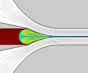
This paper analyses the effect of a soluble surfactant on the stability of the liquid–liquid hydrodynamic focusing configuration sketched in figure 1, commonly referred to as flow focusing. In this axisymmetric configuration, a liquid of density  $\rho _i$ and viscosity $\mu _i$ is injected at a constant flow rate $Q_i$ across a cylindrical feeding capillary of radius $\hat {R}_c$. This liquid flows surrounded by an outer liquid current of density $\rho _o$ and viscosity $\mu _o$, immiscible with the former. The outer current is injected at a constant flow rate $Q_o$ across a converging nozzle concentric with the inner one. The inner and outer phases coflow through the nozzle, which ends in a tube with diameter $\hat {D}$. The surface tension without surfactant is $\hat {\gamma }_*$. As explained below, we will use this value as the characteristic surface tension $\hat {\gamma }_c$.

Figure 1. Sketch of the fluid configuration.
Under certain parameter conditions, the system adopts the microjetting mode of tip streaming (Montanero & Gañán-Calvo Reference Montanero and Gañán-Calvo2020). In this mode, a jet with a diameter much smaller than  $2\hat {R}_c$ and $\hat {D}$ is emitted from the tip of the fluid meniscus attached to the feeding capillary. The jet and the outer stream coflow through the discharge tube (figure 1). The jet is expected to break up into droplets beyond the fluid domain considered in our analysis. The stability of microjetting in a similar flow focusing configuration was studied by Cabezas et al. (Reference Cabezas, Rubio, Rebollo-Muñoz, Herrada and Montanero2021) both experimentally and numerically. The results of the global stability analysis were in good agreement with the experiments.
The geometry considered in the present work is the same as that analysed by Cabezas et al. (Reference Cabezas, Rubio, Rebollo-Muñoz, Herrada and Montanero2021) except that it incorporates a discharge cylindrical tube (marked with a red line in figure 1) not considered in that work. In this way, the inner and outer streams do not slow down beyond the nozzle neck. Perturbations growing in the tube are convected downstream. This eliminates the unstable modes associated with the jet (absolute instability) (Huerre & Monkewitz Reference Huerre and Monkewitz1990) and allows one to focus on the meniscus stability. It is known that tip streaming instability originates in the tapering meniscus in most relevant realizations (Montanero & Gañán-Calvo Reference Montanero and Gañán-Calvo2020). Therefore, the stability limit for the present configuration is not expected to differ significantly from that of the geometrical configuration analysed by Cabezas et al. (Reference Cabezas, Rubio, Rebollo-Muñoz, Herrada and Montanero2021). As shown in § 4, the flow fully develops near the tube entrance. For this reason, the spectrum of eigenvalues characterizing the linear dynamics becomes practically insensitive to the tube length for relatively small values of this parameter.
The geometry studied in this work can be regarded as a hybrid between flow focusing and confined selective withdrawal (He et al. Reference He, Campo-Cortés, Goral, López-León and Gordillo2019), where the focusing effect is produced by a cylindrical tube located in front of the feeding capillary. There are, however, noticeable differences between these two configurations. The shape of the focusing element (either an orifice or a tube) significantly affects the microjetting stability (López et al. Reference López, Cabezas, Montanero and Herrada2022).
2.2. The surfactant
This paper examines the effect of a surfactant dissolved in the inner phase on the microjetting stability. The surfactant transport across the bulk is described in terms of the diffusion coefficient  $\hat {{\mathcal {D}}}_i$. In particular, the diffusion flux normal to the interface is
 \begin{equation} \hat{{\mathcal{J}}}_{\mathcal{D}}={-}\hat{{\mathcal{D}}}_i \frac{\partial \hat{c}}{\partial n}, \end{equation}
where  $\hat {c}$ is the bulk surfactant concentration, $n$ is the direction normal to the interface and $\partial \hat {c}/\partial n$ is evaluated at the interface (the interface sublayer). The diffuse layer also depends on the ionic strength of ionic surfactants, such as sodium dodecyl sulphate (SDS). This effect is not considered in our analysis.
We adopt the kinetic model for the adsorption/desorption flux
 \begin{equation} \hat{{\mathcal{J}}}= \hat{{\mathcal{J}}}_a-\hat{{\mathcal{J}}}_d,\quad \hat{{\mathcal{J}}}_a=\hat{k}_a\hat{c}_s\left(1- \frac{\hat{\varGamma}}{\hat{\varGamma}_{\infty}}\right),\quad \hat{{\mathcal{J}}}_d=\hat{k}_d \hat{\varGamma}, \end{equation}
where  $\hat {{\mathcal {J}}}$ is the net sorption flux, $\hat {{\mathcal {J}}}_a$ and $\hat {{\mathcal {J}}}_d$ are the adsorption and desorption fluxes, respectively, $\hat {k}_a$ and $\hat {k}_d$ are the adsorption and desorption constants, respectively, $\hat {c}_s$ is the bulk surfactant concentration $\hat {c}$ evaluated at the interface, $\hat {\varGamma }$ is the surfactant surface concentration (the surface coverage, measured in mols per unit area) and $\hat {\varGamma }_{\infty }$ is the maximum packing density.
The surfactant molecules absorbed on the interface are transported by convection and diffusion. The surfactant surface diffusion is determined by the surface diffusion coefficient  $\hat {{\mathcal {D}}}_{s}$, which typically takes values similar to those of the bulk diffusion coefficient $\hat {{\mathcal {D}}}_i$ (Tricot Reference Tricot1997).
We assume that the transfer of surfactant between the sublayer next to the interface and the interface occurs only in the form of monomers. This implies that  $\hat {c}$ is the volumetric concentration of monomers even if the surfactant concentration exceeds the critical micelle concentration $\hat {c}_{cmc}$ and, therefore, there are micelles in the inner liquid. Since the micelles do not contribute to $\hat {c}_s$, values of $\hat {c}_s$ exceeding the critical micelle concentration correspond to higher experimental values of the surfactant concentration. We will consider surfactant concentrations larger than $\hat {c}_{cmc}$. However, these concentrations will be sufficiently small for the dynamical effects of the micelles to be negligible.
The surfactant is convected throughout the incompressible inner liquid phase. For this reason, the surfactant concentration in the feeding capillary is approximately the same as that in the reservoir,  $\hat {c}_\infty$. The bulk diffusion coefficient $\hat {{\mathcal {D}}}_i$ corresponds to very high values of the Péclet number in most experiments. This implies that the bulk surfactant concentration is almost uniform in the inner phase, except within a thin diffusive layer of thickness $\hat {\lambda }_D$ next to the interface.
As shown in § 4,  $\hat {\lambda }_D/\hat {R}_c\sim 10^{-3}$ for the values of $\hat {{\mathcal {D}}}_i$, $\hat {k}_a$ and $\hat {R}_c$ of the reference case studied in §§ 4–6. The disparity between the thickness of the diffusive layer next to the interface and the relevant dimensions of the problem poses a major challenge to the numerical simulation. This challenge can be circumvented by assuming the approximation $\hat {c}_s\sim \hat {c}_{\infty }$, which leads to accurate results under certain conditions (Lytra et al. Reference Lytra, Vlachomitrou and Pelekasis2024). As explained in § 3, we resolve the surfactant mass boundary layer by using a spatial discretization based on Chebyshev spectral collocation points (Khorrami Reference Khorrami1989).
The effect of the surface concentration  $\hat {\varGamma }$ on the surface tension $\hat {\gamma }$ is described by the Langmuir equation of state (Tricot Reference Tricot1997)
 \begin{equation} \hat{\gamma}=\hat{\gamma}_*+\hat{\varGamma}_{\infty} \hat{R}_g T\ln \left(1-\frac{\hat{\varGamma}}{\hat{\varGamma}_{\infty}}\right), \end{equation}
where  $\hat {R}_g$ is the gas constant and $T$ is the temperature. This equation can be derived from (2.2a–c) and the Gibbs isotherm (Chang & Franses Reference Chang and Franses1995). The surface tension variation over the interface gives rise to the local soluto-capillarity effect and Marangoni stress.
As mentioned in the Introduction, we do not consider surface rheology effects. The effects of the shear  $\mu _1^S$ and dilatational $\mu _2^S$ surface viscosities can be quantified in terms of the superficial Ohnesorge numbers $Oh_{1,2}^S=\mu _{1,2}^S(\rho _i \hat {\gamma }_c \hat {R}_c^3)^{-1/2}$, which measure the relative importance of the surface viscous stresses and the capillary pressure. Ponce-Torres et al. (Reference Ponce-Torres, Rubio, Herrada, Eggers and Montanero2020) concluded that the SDS viscosities are at most of the order of $10^{-7}\ {\rm Pa} \,{\cdot }\, {\rm s} \,{\cdot }\, {\rm m}$. Then, the Ohnesorge numbers are at most of the order of $10^{-2}$ in our problem, which indicates that SDS surface viscosities can be neglected.
2.3. Dimensionless numbers
We choose the feeding capillary radius  $\hat {R}_c$, the visco-capillary velocity $v_{\gamma \mu }=\hat {\gamma }_c/\mu _i$ and the capillary pressure $\hat {\gamma }_c/\hat {R}_c$ as the characteristic quantities, where $\hat {\gamma }_c$ is a characteristic value of the surface tension, whose choice will be discussed below.
In the absence of surfactants, the problem can be formulated in terms of the density and viscosity ratios,  $\rho =\rho _o/\rho _i$ and $\mu =\mu _o/\mu _i$, the Ohnesorge and capillary numbers
 \begin{equation} {Oh}_i=\left(\frac{\mu_i}{\rho_i v_{\gamma\mu} \hat{R}_c}\right)^{1/2}=\frac{\mu_i}{(\rho_i \hat{\gamma}_c \hat{R}_c)^{1/2}} \quad \text{and} \quad \textit{Ca}=\frac{\mu_o U}{\hat{\gamma}_c}, \end{equation}
and the flow rate ratio  $Q=Q_i/Q_o$. Here, $U=4Q_o/({\rm \pi} \hat {D}^2)$ is the mean velocity in the nozzle neck. The capillary number is the ratio of the characteristic viscous stress $\mu _o U/\hat {R}_c$ to the capillary pressure $\hat {\gamma }_c/\hat {R}_c$.
When a soluble surfactant is added to the disperse phase, the following dimensionless numbers are considered as well: the bulk and surface Péclet numbers  ${Pe}=\hat {R}_cv_{\gamma \mu }/\hat {{\mathcal {D}}}_i$ and ${Pe}_s=\hat {R}_cv_{\gamma \mu }/\hat {{\mathcal {D}}}_s$, the dimensionless adsorption and desorption constants $k_a=\hat {k}_a \hat {c}_{cmc} \hat {R}_c/(\hat {\varGamma }_{\infty }v_{\gamma \mu })$ and $k_d=\hat {k}_d \hat {R}_c/v_{\gamma \mu }$, the Marangoni (elasticity) number $Ma=\hat {\varGamma }_{\infty } R_g T/\hat {\gamma }_c$ and the reservoir surfactant concentration $c_\infty =\hat {c}_\infty /\hat {c}_{cmc}$.
There are two natural choices for the characteristic surface tension: (i) the value  $\hat {\gamma }_*$ corresponding to the surfactant-free case and (ii) the equilibrium value $\hat {\gamma }_{eq}$ corresponding to reservoir concentration $\hat {c}_\infty$. As shown in § 4, surfactant molecules are convected downstream by the interface, which results in values of the meniscus surface tension much larger than $\hat {\gamma }_{eq}$. For this reason, we consider $\hat {\gamma }_*$ in the definition of the dimensionless numbers.
For a fixed geometry, the set of dimensionless numbers governing the problem is  $\{\rho$, $\mu$, Oh $_i$,
$_i$,  ${\textit {Ca}}$, $Q$;
$Q$;  $Pe, Pe_s$, $k_a$, $k_d$, $Ma$,
$Ma$,  $c_\infty \}$. In a typical experimental run, the microfluidic device, the fluids and the surfactant are fixed. For this reason, the variables $Ca$ and $Q$ can be regarded as the control parameters. To determine the stability limit, one selects the outer flow rate $Q_o$ and progressively decreases the inner flow rate $Q_i$ until its minimum value $Q_{i\,{min}}$ for microjetting is reached. The experiment is usually repeated for several values of $Q_o$. Therefore, the goal is to determine the dimensionless minimum flow rate $Q_{min}=Q_{i\,{min}}/Q_o$ as a function of ${\textit {Ca}}$. In the presence of a surfactant, the function $Q_{min}=Q_{min}(Ca)$ must be obtained for different values of $c_\infty$ (see § 7).
3. Governing equations and numerical method
This paper analyses numerically the stability of liquid–liquid flow focusing in a converging nozzle when a surfactant is dissolved in the inner phase. For this purpose, we consider the full hydrodynamic equations, including inertia, without any approximations relative to the surfactant transport. The dimensionless Navier–Stokes equations for the axisymmetric velocity  $\boldsymbol {v}^{(k)}(r,z;t)$ and pressure $p^{(k)}(r,z;t)$ fields are
 $$\begin{gather} (ru^{(k)})_r+rw^{(k)}_z=0, \end{gather}$$
 $$\begin{gather}\rho^{\delta_{ko}} ({Oh}_i)^{{-}2}\left(\frac{\partial u^{(k)}}{\partial t} + u^{(k)} u^{(k)}_r+ w^{(k)} u^{(k)}_z\right)={-}p^{(k)}_r+\mu^{\delta_{ko}} (u^{(k)}_{rr}+(u^{(k)}/r)_r+u^{(k)}_{zz}), \end{gather}$$
 $$\begin{gather}\rho^{\delta_{ko}} ({Oh}_i)^{{-}2}\left(\frac{\partial w^{(k)}}{\partial t} + u^{(k)} w^{(k)}_r+ w^{(k)}w^{(k)}_z\right) ={-}p^{(k)}_z+\mu^{\delta_{ko}} (w^{(k)}_{rr}+w^{(k)}_r/r+w^{(k)}_{zz}), \end{gather}$$
where  $t$ is the time, $r$ (
$r$ ( $z$) is the radial (axial) coordinate, $u^{(k)}$ ( $w^{(k)}$) is the radial (axial) velocity component and $\delta _{ko}$ is the Kronecker delta. In the above equations and henceforth, the superscripts $k=i$ and $o$ refer to the inner and outer phases, respectively. In addition, the subscripts $r$ and $z$ denote the partial derivatives with respect to the corresponding coordinates. The action of the gravitational field has been neglected due to the smallness of the fluid configuration.
The velocity field is continuous at the interface, i.e.
 \begin{equation} \boldsymbol{v}^{(i)}=\boldsymbol{v}^{(o)}, \end{equation}
at  $r=F(z,t)$, where $F(z,t)$ is the distance of an interface element to the symmetry axis (figure 2). The kinematic compatibility at the interface yields
 \begin{equation} \frac{\partial F}{\partial t}+F_z w^{(i)}-u^{(i)}=0.\end{equation}
The equilibrium of normal stresses on that surface leads to
 \begin{equation} {-}p^{(i)}+\tau_n^{(i)}=\gamma\kappa-p^{(o)}+\tau_n^{(o)}, \end{equation}
where  $\gamma =\hat {\gamma }/\hat {\gamma }_*$ is the normalized surface tension
 \begin{equation} \kappa=\frac{FF_{zz}-1-F_z^{2}}{F(1+F_z^{2})^{3/2}}, \end{equation}
is the local mean curvature and
 $$\begin{gather} \tau_n^{(i)}=\frac{2[u^{(i)}_r-F_z(w^{(i)}_r+u^{(i)}_z) +F_z^{2}w^{(i)}_z]}{1+F_z^{2}}, \end{gather}$$
 $$\begin{gather}\tau_n^{(o)}=\frac{2\mu[u^{(o)}_r-F_z(w^{(o)}_r +u^{(o)}_z)+F_z^{2}w^{(o)}_z]}{1+F_z^{2}}, \end{gather}$$
are the inner and outer normal viscous stresses, respectively. The equilibrium of tangential stresses yields
 \begin{equation} \tau_t^{(i)}+\tau^{Ma}=\tau_t^{(o)}, \end{equation}
where  $\tau _t^{(i)}$ is the inner tangential viscous stress, $\tau ^{Ma}$ is the Marangoni stress and $\tau _t^{(o)}$ is the outer tangential viscous stress given by the expressions
 $$\begin{gather} \tau_t^{(i)}=(1-F_z^{2})(w^{(i)}_r+u^{(i)}_z)+2F_z(u^{(i)}_r-w^{(i)}_z), \end{gather}$$
 $$\begin{gather}\tau^{Ma}={-}\gamma_z(1+F_z^{2})^{1/2}, \end{gather}$$
 $$\begin{gather}\tau_t^{(o)}=\mu[(1-F_z^{2})(w^{(o)}_r+u^{(o)}_z)+2F_z(u^{(o)}_r-w^{(o)}_z)]. \end{gather}$$
As mentioned in § 2, the viscous surface stresses have been neglected in (3.6) and (3.10).
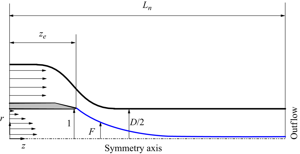
Figure 2. Sketch of the computational domain.
The surfactant volumetric concentration (measured in terms of the critical micelle concentration)  $c^{(i)}({\boldsymbol r},t)$ is calculated from the conservation equation (Craster, Matar & Papageorgiou Reference Craster, Matar and Papageorgiou2009; Kalogirou & Blyth Reference Kalogirou and Blyth2019)
 \begin{equation} \frac{\partial c^{(i)}}{\partial t}+u^{(i)} c^{(i)}_r+w^{(i)} c^{(i)}_z={Pe}^{{-}1}[(r c^{(i)}_{r})_r/r+c^{(i)}_{zz}]. \end{equation}
We assume that monomers are at equilibrium with micelles at concentrations exceeding the critical micelle concentration. Therefore, the net flux of micelle formation/destruction vanishes.
The net sorption flux  ${\mathcal {J}}=\hat {{\mathcal {J}}}\hat {R}_c/(v_{\gamma \mu }\hat {\varGamma }_{\infty })$ at the interface is calculated as (2.2a–c) (Craster et al. Reference Craster, Matar and Papageorgiou2009; He et al. Reference He, Yazhgur, Salonen and Langevin2015; Kalogirou & Blyth Reference Kalogirou and Blyth2019)
 \begin{equation} {\mathcal{J}}={\mathcal{J}}_a-{\mathcal{J}}_d,\quad {\mathcal{J}}_a=k_a c^{(i)}_s(1-\varGamma),\quad {\mathcal{J}}_d=k_d\varGamma, \end{equation}
where  ${\mathcal {J}}_a=\hat {{\mathcal {J}}_a}\hat {R}_c/(v_{\gamma \mu }\hat {\varGamma }_{\infty })$ and ${\mathcal {J}}_d=\hat {{\mathcal {J}}_d}\hat {R}_c/(v_{\gamma \mu }\hat {\varGamma }_{\infty })$ are the dimensionless adsorption and desorption fluxes, respectively, $c^{(i)}_s$ is the surfactant concentration evaluated at the interface and $\varGamma =\hat {\varGamma }/\hat {\varGamma }_{\infty }$ is the dimensionless surfactant surface concentration. The net sorption flux equals the surfactant diffused from/to the bulk ${\mathcal {J}}_{\mathcal {D}}$; i.e.
 \begin{equation} {\mathcal{J}}={\mathcal{J}}_{\mathcal{D}}=\left.\frac{c^{(i)}_z F_z-c^{(i)}_r}{{Pe}\sqrt{1+F_z^2}}\right|_{r=F}. \end{equation}
This equation couples surfactant transport across the bulk and over the interface.
The surfactant surface concentration  $\varGamma$ satisfies the advection–diffusion equation (Craster et al. Reference Craster, Matar and Papageorgiou2009)
 \begin{equation} \frac{\partial \varGamma}{\partial t}+{\boldsymbol \nabla}_s\boldsymbol{\cdot}(\varGamma {\boldsymbol v}_s)+\varGamma \kappa ({\boldsymbol v}\boldsymbol{\cdot}{\boldsymbol n})=\frac{1}{{Pe}_s}\boldsymbol{\nabla}_s^2 \varGamma+{\mathcal{J}}, \end{equation}
where  ${\boldsymbol v}_s={\boldsymbol {\textsf I}}_s{\boldsymbol v}=v_s {\boldsymbol t}$ is the (two-dimensional) surface velocity, ${\boldsymbol t}$ is the tangential unit vector, ${\boldsymbol {\textsf I}}_s={\boldsymbol {\textsf I}}-{\boldsymbol n}{\boldsymbol n}$ is the tensor that projects any vector on that surface, ${\boldsymbol {\textsf I}}$ is the identity tensor, ${\boldsymbol n}$ is the unit outward normal vector and ${\boldsymbol \nabla _s}$ is the tangential intrinsic gradient along the free surface parametrized with the intrinsic coordinate $s$. The above equation can be re-written as
 $$\begin{gather} \frac{\partial \varGamma}{\partial t}+\varGamma \left(\frac{{\rm d} v_s}{{\rm d} s}+\frac{{\rm d} F/{\rm d} s}{F}v_s\right)+ \frac{{\rm d} \varGamma}{{\rm d} s}v_s+\varGamma \kappa ({\boldsymbol v}\boldsymbol{\cdot}{\boldsymbol n})=\frac{1}{{Pe}_s}\left(\frac{{\rm d}^2\varGamma}{{\rm d} s^2}+\frac{{\rm d} \varGamma}{{\rm d} s}\, \frac{{\rm d} F/{\rm d} s}{F}\right)+{\mathcal{J}}, \end{gather}$$
 $$\begin{gather}v_s=\frac{w^{(i)}+F_z u^{(i)}}{(1+F_z^2)^{1/2}}, \quad {\boldsymbol v}\boldsymbol{\cdot}{\boldsymbol n}=\frac{u^{(i)}-F_z w^{(i)}}{(1+F_z^2)^{1/2}}, \quad\frac{{\rm d} A}{{\rm d} s}=\frac{A_z}{(1+F_z^2)^{1/2}}, \end{gather}$$
where  $A$ is any scalar quantity.
The dependence of the surface tension  $\gamma$ upon the surfactant surface concentration $\varGamma$ is calculated from the Langmuir equation of state (2.3) (Tricot Reference Tricot1997), which in dimensionless form is
 \begin{equation} \gamma=1+ {Ma} \log(1-\varGamma).\end{equation}
The hydrodynamic equations are integrated within the numerical domain sketched in figure 2. We prescribe a parabolic velocity distribution at the inlet section of the feeding capillary, while a uniform velocity profile is imposed at the inlet section of the outer tube. This approximately corresponds to many flow focusing experiments in which a short nozzle is connected to a large tank to drive the outer fluid. Conversely, the inner feeding capillary is usually very long in terms of its diameter.
We consider the no-slip boundary condition at the solid walls and the outflow conditions  $u^{(k)}_z=w^{(k)}_z=F_z=0$ at the right-hand end of the computational domain ( $F_z=0$ only holds at the interface). The anchorage condition of the triple contact line, $F=1$, is imposed at the edge of the feeding capillary. The reservoir surfactant concentration $c_\infty$ is imposed at the inlet section of the feeding capillary. The numerical integration of (3.17) is performed considering zero surfactant diffusive flux at the triple contact line and the outlet section. We consider the standard regularity conditions $u^{(i)}=w^{(i)}_r=c^{(i)}_r=0$ at the symmetry axis.
In the global stability analysis, we assume the temporal dependence
 \begin{equation} \left.\begin{array}{c} U(r,z;t)=U_0(r,z)+\delta U(r,z)\, {\rm e}^{-{\rm i}\omega t}+\text{c.c.} \quad (|\delta U|\ll U_0), \\ F(z;t)=F_0(z)+\delta F(z)\, {\rm e}^{-{\rm i}\omega t}+\text{c.c.}\quad (|\delta F|\ll F_0),\\ \varGamma(z;t)=\varGamma_0(z)+\delta \varGamma(z)\, {\rm e}^{-{\rm i}\omega t}+\text{c.c.}\quad (|\delta \varGamma|\ll \varGamma_0), \end{array}\right\} \end{equation}
where  $U(r,z;t)$ represents the velocity, pressure and bulk surfactant concentration fields, while $U_0(r,z)$ and $\delta U(r,z)$ stand for the base flow (steady) solution and the spatial dependence of the eigenmode, respectively. In addition, $F_0(z)$ and $\varGamma _0(z)$ represent the base flow solution for $F(z)$ and $\varGamma (z)$, respectively, while $\delta F$ and $\delta \varGamma$ are the corresponding perturbation amplitudes. The perturbation evolves according to the eigenfrequency $\omega =\omega _r+\textrm {i}\omega _i$, where $\omega _r$ and $\omega _i$ are the oscillation frequency and growth rate, respectively. The flow asymptotic linear stability (Theofilis Reference Theofilis2011) is determined by the eigenfrequency $\omega ^*=\omega _r^*+\textrm {i}\omega _i^*$ of the dominant mode (that with the largest growth rate). Microjetting realizations with $\omega _i^*<0$, $\omega _i^*=0$ and $\omega _i^*>0$ correspond to stable, marginally stable and unstable flows, respectively.
As observed in (3.21), we restrict ourselves to axisymmetric perturbations, which are known to be dominant in experiments. In fact, non-axisymmetric instability appears only for sufficiently large aerodynamic Weber numbers We $=\rho _o (U-v_j)^2 d_j/\hat {\gamma }_c$ defined in terms of the mean jet and outer stream velocities, $v_j$ and $U$, and the jet diameter $d_j$. This instability cannot occur in our configuration. The low value of the Reynolds number ensures that the flow adopts the Poiseuille solution practically at the entrance of the discharge tube (figure 7), and the aerodynamic Weber number equals 0.054.
The governing equations are integrated with a variant of the numerical method proposed by Herrada & Montanero (Reference Herrada and Montanero2016) and Herrada (Reference Herrada2023). This method, as applied to liquid–liquid flow focusing without surfactant, was explained in detail by Cabezas et al. (Reference Cabezas, Rubio, Rebollo-Muñoz, Herrada and Montanero2021). As mentioned in § 2, the major difficulty associated with a soluble surfactant is the existence of a very thin diffusive boundary layer next to the interface for the small diffusion coefficients of most surfactants. However, using Chebyshev spectral collocation points to discretize the radial direction accumulates the grid points next to the interface (Herrada & Montanero Reference Herrada and Montanero2016), facilitating the resolution of this layer (figure 3).

Figure 3. Detail of the grid used in the simulations.
The inner and outer fluid domains were mapped onto two quadrangular domains through a non-singular mapping. The shape functions were obtained as a part of the solution by using a quasi-elliptic transformation (Dimakopoulos & Tsamopoulos Reference Dimakopoulos and Tsamopoulos2003). Some additional boundary conditions for the shape functions were needed to close the problem. All the derivatives appearing in the governing equations were expressed in terms of the spatial coordinates  $(\chi,\xi )$ resulting from the mapping. These equations were discretized in the (mapped) radial direction with $n_{\chi }^{i}=n_{\chi }^{o}=50$ Chebyshev spectral collocation points (Khorrami Reference Khorrami1989) in the inner and outer domains. We used fourth-order finite differences with $n_{\xi }^{(i)}=n_{\xi }^{(o)}=4501$ equally spaced points to discretize the (mapped) axial direction in the inner and outer phases.
The Matlab Eigs function was applied to find the eigenfrequencies around a reference value  $\tilde {\omega }$. This process was repeated for several values of $\tilde {\omega }$ to obtain part of the eigenfrequency spectrum. We conducted a grid sensitivity analysis to ensure the grid size did not affect the results. We verified that the surfactant surface density, interface velocity and critical eigenfrequency differed by less than 1 % when the number of grid points was increased by 50 %.
We also conducted transient (direct) numerical simulations to show the response of the microjetting mode to an initial perturbation. The numerical method is essentially the same as that used in the stability analysis. We used the spatial discretization of the mapped numerical domain described above. The time domain was discretized with second-order backward finite differences. The time step  $\Delta t=0.5$ was constant. We verified that reducing the time step did not significantly change the results.
The rest of this paper is organized as follows. Section 4 describes the base flow for a reference case characterized by realistic values of the governing parameters. Section 5 analyses the stabilizing effect of the surfactant monolayer in that case by comparing the results with and without surfactant. Section 6 shows transient numerical simulations in the presence of the surfactant for the reference case too. § 7 explores the system's response when the surfactant parameters are changed. Finally, concluding remarks are presented in § 8.
4. Base flow of the reference case
As the reference case, we consider the configuration characterized by the following realistic parameters. The nozzle shape and the feeding capillary position are the same as those in the experiments of Cabezas et al. (Reference Cabezas, Rubio, Rebollo-Muñoz, Herrada and Montanero2021). The capillary radius is  $\hat {R}_c=0.1$ mm. In terms of this characteristic length, the relevant lengths in the simulations are $L_n=11.4$, $z_e=3.8$ and $D=2$ (figure 2). We consider the physical properties very similar to those of the water–oil system studied by Moyle et al. (Reference Moyle, Walker and Anna2012): $\rho _i=998\ \textrm {kg}\ \textrm {m}^{-3}$, $\rho _o=830\ \textrm {kg}\ \textrm {m}^{-3}$, $\mu _i=1.33\ \textrm {mPa} {\cdot } \textrm {s}$, $\mu _o=53.1\ \textrm {mPa} {\cdot } \textrm {s}$ and $\hat {\gamma }_*=62\ \textrm {mN}\ \textrm {m}^{-1}$. We consider the surfactant properties reported by Liang et al. (Reference Liang, Li, Wang and Luo2022) for SDS in a water–nOctane system: $\hat {{\mathcal {D}}}_i=7.9\times 10^{-10}\ \textrm {m}^2\ \textrm {s}^{-1}$, $\hat {{\mathcal {D}}}_s=7.9\times 10^{-10}\ \textrm {m}^2\ \textrm {s}^{-1}$, $\hat {\varGamma }_{\infty }=3.13\ \mathrm {\mu }\textrm {mol}\ \textrm {m}^{-2}$, $R_g=8.314\ \textrm {J}\ \textrm {(K mol)}^{-1}$, $\hat {k}_a=8.25\times 10^{-5}\ \textrm {m}\ \textrm {s}^{-1}$, $\hat {k}_d=1.3$ s $^{-1}$ and $\hat {c}_{cmc}=8.3\ \textrm {mol}\ \textrm {m}^{-3}$. The corresponding values of the dimensionless numbers are $\rho =0.83$, $\mu =40$, $Oh_i=0.0169$, $Pe=5.89\times 10^6$, $Pe_s=5.89\times 10^6$, $k_a=4.71\times 10^{-4}$, $k_d=2.79\times 10^{-6}$ and $Ma=0.117$. All the results were calculated for these values unless otherwise specified.
The condition  $c_{\infty }>1$ (a concentration larger than the critical micelle concentration) is necessary to observe a significant surfactant effect in the experiments (Moyle et al. Reference Moyle, Walker and Anna2012; López et al. Reference López, Cabezas, Montanero and Herrada2022). For this reason, we consider the surfactant concentration $c_{\infty }=1.47$. As explained below, this concentration is sufficiently small for the Langmuir equation to provide reliable interfacial tension values. We select the capillary number $Ca=0.349$, a similar value to those of the experiments of Cabezas et al. (Reference Cabezas, Rubio, Rebollo-Muñoz, Herrada and Montanero2021).
The results presented in this section correspond to the marginally stable ( $\omega _i=0$) case obtained for $Q=0.005$. These results are compared with those of the unstable ( $\omega _i>0$) base flow without surfactant obtained for the same values of the governing parameters.
Figure 4 shows the surfactant volumetric concentration for the reference case. Due to the small value of the diffusion coefficient, a thin mass boundary layer separates the stream coming from the feeding capillary from the recirculating cells that occupy the tapering meniscus. The surfactant is convected across a narrow annular streamtube next to the interface. The surfactant molecules adsorb onto the interface according to the kinetic model (3.15a–c). Adsorption occurs mostly next to the feeding capillary (figure 5), where the adsorption flux is higher (the interface is empty), the interface area is larger and the surface velocity is smaller.

Figure 4. Surfactant volumetric concentration  $c^{(i)}_0(r.z)$ for $Ca=0.349$, $Q=0.005$ and $c_{\infty }=1.47$. The lines are the streamlines.

Figure 5. Interface location  $F_0(z)$ (a), adsorption flux ${\mathcal {J}}^a_0(z)$, desorption flux ${\mathcal {J}}^d_0(z)$ (b), surface concentration $\varGamma _0(z)$ (c), surface tension $\gamma _0(z)$ (d) and surface velocity $v^s_0(z)$ (e) for $Ca=0.349$, $Q=0.005$, and $c_{\infty }=1.47$. The red dashed lines indicate the interface location and velocity without surfactant. Here, $z_e$ is the axial coordinate of the capillary exit.
The liquid flowing next to the interface is slightly emptied of surfactant downstream. Flow recirculation convects this small surfactant depletion throughout the tapering meniscus (figure 4). Overall, the surfactant volumetric concentration is relatively constant in the fluid domain ( $1.33\leq c^{(i)}\leq 1.47$), including the sublayer next to the interface. This behaviour was also described by Lytra et al. (Reference Lytra, Vlachomitrou and Pelekasis2024) for a similar configuration.
As mentioned above, the volumetric surfactant concentration evaluated at the free surface,  $c^{(i)}_{0s}$, practically takes the upstream value $c_{\infty }$. This can be anticipated from a simple scaling analysis. Consider the surfactant boundary layer next to the interface. According to (3.15a–c), the variation $\Delta c_0^{(i)}$ of surfactant concentration across that layer can be estimated as
 \begin{equation} \widetilde{Pe}^{{-}1} \frac{\Delta c_0^{(i)}}{\lambda_D} \sim \frac{\tilde{k}_a}{v_{\lambda}} c^{(i)}_{0s}, \end{equation}
where  $\widetilde {Pe}=\hat {v}_{\lambda }\hat {R}_c/\hat {\mathcal {D}}_i$ is the Péclet number defined in terms of the characteristic velocity $\hat {v}_{\lambda }$ in the surfactant boundary layer, $\lambda _D\sim \widetilde {Pe}^{-1/2}$ is the (dimensionless) boundary layer thickness (Levich Reference Levich1962), $\tilde {k}_a=\hat {k}_a/v_{\gamma \mu }$ and $v_{\lambda }=\hat {v}_{\lambda }/v_{\gamma \mu }$. The order of magnitude of the ratio $\Delta c_0^{(i)}/c^{(i)}_{0s}$ is
 \begin{equation} \frac{\Delta c_0^{(i)}}{c^{(i)}_{0s}}\sim \frac{\tilde{k}_a}{v_{\lambda}} \widetilde{Pe}^{1/2}. \end{equation}
The Schmidt number Sc $=\mu _i/\rho _i \hat {\mathcal {D}}_i$ is of the order of $10^3$, which implies that $\lambda _D$ is much smaller than the characteristic viscous diffusion length. For this reason, we can assume that $v_{\lambda }\sim v_{0}^s\sim 10^{-2}$ (figure 5). This implies that $\widetilde {Pe}\sim 10^5$, $\lambda _D\sim 10^{-3}$– $10^{-2}$ and $\Delta c^{(i)}/c^{(i)}_{0s}\sim 10^{-2}$– $10^{-1}$, which is consistent with the numerical results. We conclude that convection ensures $c^{(i)}_{0s}\simeq c_{\infty }$ throughout the inner fluid domain. This constitutes an advantage numerically because it makes discretization errors in the boundary layer less relevant.
As mentioned above, adsorption occurs mostly next to the feeding capillary. However, a sharp reduction of the interface radius occurs in the meniscus tip. The reduction of the interface area considerably increases the surfactant surface concentration there (figure 5). The increase in the surfactant surface concentration leads to a significant decrease in the surface tension (figure 5).
The residence time of the interface element in the meniscus tip takes relatively small values due to the higher surface velocities there. This effect hinders surfactant desorption, which is almost negligible throughout the interface (figure 5) even though the surfactant surface density approaches the maximum packing density in the meniscus tip (figure 5).
The surfactant concentration  $c_{\infty }=1.47$ leads to the surface coverage $\varGamma _{eq}=0.997$ at equilibrium, which would render the Langmuir model inaccurate. However, the surfactant molecules are convected downstream in the present dynamical problem, which significantly reduces the surface coverage and allows one to use the Langmuir equation of state safely even for concentrations higher than the critical micelle concentration. In fact, $c_{\infty }=1.47$ leads to surface tension reduction in our simulation smaller than 30 % (figure 5), much smaller than that at equilibrium for the same concentration (Liang et al. Reference Liang, Li, Wang and Luo2022).
The Marangoni stress in the meniscus tip acts against the viscous drag exerted by the outer flow. This substantially alters the balance of the tangential stresses at the interface. Specifically, the viscous drag exerted by the outer stream increases in the presence of surfactant (figure 6). However, the momentum transfer to the inner phase is slightly smaller. As explained in § 5, the decrease in the inner-phase flow rate dragged by the outer current stabilizes the flow. The increase in the viscous drag exerted by the external stream entails an increase in the pressure drop driving the outer phase.

Figure 6. Interface location  $F_0(z)$ and tangential stress at the interface: outer viscous stress $\tau _{t0}^{(o)}$, inner viscous stress $\tau _{t0}^{(i)}$ and Marangoni stress $\tau _0^{Ma}$. The results were calculated for $Ca=0.349$, $Q=0.005$ and $c_{\infty }=0$ (a) and 1.47 (b).
The surface velocity  $v_s$ is of the order of the mean velocity in the nozzle neck, which implies that $v_s\sim {Ca}/\mu \sim 10^{-2}$, as shown below. Interestingly, the Marangoni stress magnitude is insufficient to reduce the surface velocity. Figures 5 and 6 show that Marangoni stress tries to immobilize the interface in the meniscus tip, where the surface tension gradient takes higher values. However, the flow practically develops at the entrance of the nozzle neck due to the large viscosity forces (figure 7). The value of $v_s$ downstream is fixed by the Hagen–Poiseuille parabolic profiles, which are unaffected by the surfactant. Therefore, $v_s(z)$ takes practically the same value with and without surfactant. This behaviour substantially differs from that observed in open flows, where the Marangoni stress reduces the interface velocity and, therefore, the intensity of the inner flow (Frumkin & Levich Reference Frumkin and Levich1947; Herrada et al. Reference Herrada, Ponce-Torres, Rubio, Eggers and Montanero2022).

Figure 7. Axial velocity profile,  $w_0^{(i)}$ and $w_0^{(o)}$, at the nozzle sections $z-z_e=3.6$, 4.2, 5.6 and 7.6. The results were calculated for $Ca=0.349$, $Q=0.005$ and $c_{\infty }=1.47$. The inset shows the nozzle sections corresponding to the velocity profiles.
The jet radius  $R_j$, the pressure gradient $K$ and the interface velocity $v_s$ in the discharge tube are approximately given by the fully developed flow formulae
 $$\begin{gather} R_j=\left(\frac{Q}{1+Q+\sqrt{1+Q\mu}}\right)^{1/2}, \end{gather}$$
 $$\begin{gather}K={-}8 Ca \mu^{{-}2} [2+\mu(Q+\mu-2)+2(\mu-1)\sqrt{1+Q\mu}], \end{gather}$$
and
 \begin{equation} v_s=2 Ca \mu^{{-}2}(\mu-1+\sqrt{1+Q\mu}). \end{equation}
The values of  $R_j$ and $v_s$ evaluated at the outlet of the numerical domain are 0.04859 and 0.01747, respectively, while the corresponding analytical predictions (4.3)–(4.5) are 0.04879 and 0.01749. Equation (4.3) shows that the jet diameter $d_j$ scales as $Q_i^{1/2}$ for $Q\ll 1$ and $Q\mu \ll 1$. It is worth mentioning that the condition $Q\mu \ll 1$ does not verify in our simulations even though $Q\ll 1$. For instance, $Q\mu =0.2$ and 0.5 at the stability limit with and without surfactant, respectively.
As mentioned above, the surfactant accumulates in the meniscus tip interface. The surfactant effect is localized in that region. For this reason, the base flows with and without surfactant are similar on the scale given by the feeding capillary radius (figure 8). In particular, the surfactant monolayer does not significantly alter the interface location  $F_0(z)$. The surfactant slightly reduces the recirculation cell size, making the stagnation point in the meniscus tip move upstream (figure 9). However, the surfactant hardly affects the upstream stagnation point location. This indicates that the stabilization caused by the surfactant (see § 5) is not related to the penetration of the recirculation cell into the feeding capillary, a destabilizing mechanism in gaseous flow focusing (Montanero & Gañán-Calvo Reference Montanero and Gañán-Calvo2020).

Figure 8. Streamlines for  $Ca=0.349$, $Q=0.005$ and $c_{\infty }=0$ (a) and 1.47 (b). The colour indicates the velocity magnitude in terms of the mean velocity in the discharge tube $U$.
$U$.

Figure 9. Interface location  $F_0(z)$, (a) hydrostatic pressure $p_0^{(i)}$ (b) and velocity $v_0^{(i)}$ (c) at the symmetry axis. The results were calculated for $Ca=0.349$, $Q=0.005$ and $c_{\infty }=0$ and 1.47. The dashed vertical lines indicate the position of the stagnation points. The dotted line indicates the pressure drop (4.4) corresponding to fully developed flow with constant surface tension.
As explained in § 5, the instability originates in the meniscus–jet transition region. The decrease in capillary pressure caused by the surfactant monolayer in that region considerably reduces the pressure force opposing the flow (figure 9). This partially explains why the surfactant stabilizes the flow. We will return to this in § 5.
5. Linear stability analysis of the reference case
This section analyses the linear stability of the reference case considered in the previous section. We explain how the surfactant monolayer stabilizes the flow by studying its effect on the perturbations and the base flow separately.
As explained in § 2, the set of dimensionless parameters characterizing the present problem are
 \begin{equation} \{\rho,\mu,{Oh}_i,Ca,Q;{Pe},{Pe}_s,k_a,k_d, {Ma},c_\infty\}. \end{equation}
The subset
 \begin{equation} \{{\mathcal{P}}_i\}\equiv \{{Pe},{Pe}_s,k_a,k_d, {Ma},c_\infty\}, \end{equation}
accounts for the surfactant effect. The linearized equations governing the perturbations depend on both  $\{{\mathcal {P}}_i\}$ and the base flow $\varPhi _0$ around which those equations are linearized. As shown in § 5, the surfactant monolayer affects the base flow $\varPhi _0$. This means that the perturbations $\delta \varPhi$ depend on $\{{\mathcal {P}}_i\}$ through (i) the dependence of the linearized equations on $\{{\mathcal {P}}_i\}$ and (ii) the dependence of the base flow $\varPhi _0$ on those parameters. In this sense, $\delta \varPhi$ obeys the formal relationship $\delta \varPhi ={\mathcal {F}}(\{{\mathcal {P}}_i\},\varPhi _0(\{{\mathcal {P}}_i\}))$. We start our analysis by considering in § 5.1 the combined influence of these two factors. Section 5.2 examines the effect of the surfactant on the perturbations exclusively (for a given base flow). Finally, we discuss the secondary role of the base flow in § 5.3.
5.1. Surfactant effect on the perturbations and base flow
The surfactant influence on the system stability through both the perturbations and the base flow can be studied by comparing the results with and without surfactant. In other words, we compare the solutions for  $c_\infty =0$ and $c_\infty =1.47$. Figure 10 shows the spectrum of eigenvalues in these two cases. The values for $\gamma =1$ (without soluto-capillarity) and $\tau ^{Ma}=0$ (without Marangoni stress) correspond to $c_\infty =0$, while the values for $\gamma \neq 1$ and $\tau ^{Ma}\neq 0$ correspond to $c_\infty =1.47$. The addition of surfactant stabilizes the microjetting mode of flow focusing, significantly reducing the critical growth rate. The eigenfrequencies of the subdominant modes are hardly affected by the surfactant monolayer. This means that the major effect of the surfactant monolayer on the system's linear dynamics occurs precisely through the critical eigenmode. This effect significantly affects the stability limit. The minimum flow rate ratio in the absence of surfactant $Q_{min}=0.0125$ decreases to 0.005 when the surfactant is added.

Figure 10. Spectrum of eigenvalues around  $\tilde {\omega }=0.6$ for $Ca=0.349$ and $Q=0.005$. The stars are the results when neither soluto-capillarity nor Marangoni stress is considered. The triangles are the results obtained only considering soluto-capillarity. The squares are the results obtained only considering Marangoni stress. The circles correspond to the results when the two effects are considered. The arrows indicate the displacement of the critical mode eigenvalue due to soluto-capillarity and Marangoni stress. The values of $Ca$ and $Q$ approximately correspond to marginal stability ( ${max}\{\omega _i\}=0$) in the presence of surfactant. The eigenvalues have been made dimensionless with the inertio-capillary time $t_{ic}=(\rho _i \hat {R}_c^3/\gamma _*)^{1/2}$.
A supercritical oscillatory Hopf bifurcation ( $\omega _r^*\neq 0$) causes the flow instability, as in most tip streaming configurations (Montanero & Gañán-Calvo Reference Montanero and Gañán-Calvo2020). The presence of the surfactant monolayer does not alter this result. The critical perturbation oscillation is linked to the presence of the jet. The jet convects capillary modes, translating into an oscillatory behaviour in the Eulerian frame of reference. As in other tip streaming configurations, $\omega _r^*$ is commensurate with the inverse of the inertio-capillary time based on the meniscus size.
The importance of soluto-capillarity and Marangoni stress has been assessed separately by ‘turning off’ the corresponding terms in the interface boundary conditions (3.6) and (3.10). When both soluto-capillarity ( $\gamma \neq 1$) and Marangoni stress ( $\tau ^{Ma}\neq 0$) are present, $Q_{min}$ decreases from 0.0125 to 0.005. If the dependence $\gamma (\varGamma )$ is retained in (3.6) but the term $\tau ^{Ma}$ is set to 0 in (3.10), $Q_{min}$ decreases from 0.0125 to 0.0075. This means that the two factors significantly contribute to the microjetting stabilization. As expected, there is a correspondence between the magnitude of the decrease in the minimum flow rate due to those factors and the corresponding decrease in the critical growth rate (figure 10): the larger the decrease in $Q_{min}$ associated with either soluto-capillarity or Marangoni stress, the larger the corresponding decrease in $\omega ^*_i$.
The surfactant monolayer not only affects the minimum flow rate ratio but also influences the shape of the interface deformation caused by the critical eigenmode. Figure 11 compares  $\delta F(z)$ for $c_{\infty }=0$ and 1.47 at the corresponding stability limit. The jet diameter is larger without surfactant because the flow rate ratio is larger in that case. The surfactant monolayer increases the interface deformation in the meniscus–jet transition region. This deformation expands upstream and downstream in the absence of surfactant.

Figure 11. Interface location  $F_0(z)$ (a) and perturbation of the interface location, $\delta F(z)$, (b) for $Ca=0.349$ and $c_{\infty }=0$ and 1.47. The results correspond to the minimum flow rate ratios $Q=0.0125$ and 0.005 corresponding to $c_{\infty }=0$ and 1.47, respectively. The values of Re[ $\delta F$] are normalized by dividing them by the absolute values of the corresponding minimum values.
5.2. Surfactant effect on the perturbations
In the previous section, we analysed the influence of the surfactant on the microjetting stability through its effect on both the perturbations and the base flow. Now, we exclusively examine the surfactant effect on the perturbations, i.e. for a given base flow. Specifically, we consider the marginally stable base flow for  $c_{\infty }=1.47$ and study the perturbations around this base flow with and without the surfactant effect only on the perturbations (not on the base flow).
In the presence of a surfactant monolayer, the perturbation produces a variation  $\delta \gamma (z)\, \textrm {e}^{-\textrm {i}\omega t}+\textrm {c.c.}$ of the surface tension with respect to its value $\gamma _0(z)$ in the base flow. This variation is the distinct feature of the perturbations suffered by a surfactant-loaded interface. For this reason, we analyse its effect on the spectrum of eigenfrequencies. The amplitude $\delta \gamma$ can be calculated from the linearization of (3.20) as $\delta \gamma =- {Ma} \delta \varGamma$.
The linearized equation for the balance of normal stresses at the interface reads
 \begin{equation} {-}\delta p^{(i)}+\delta\tau_n^{(i)}=\gamma_0 \delta\kappa+\delta p_{\gamma}-\delta p^{(o)}+\delta\tau_n^{(o)}, \end{equation}
where  $\delta p^{(i)}$, $\delta p^{(o)}$, $\delta \tau _n^{(i)}$ and $\delta \tau _n^{(o)}$ are the perturbations of the hydrostatic pressure and normal viscous stresses, $\gamma _0(z)$ is the surface tension in the base flow and
 \begin{align} \delta\kappa&=\frac{1}{F_0^2\sqrt{1+F_{0z}^2}}\delta F+\frac{F_0 F_{0z}+F_0 F_{0z}^3-3 F_0^2 F_{0z} F_{0zz}}{F_02(1+F_{0z}^2)^{5/2}} \delta F_z\nonumber\\ &\quad +\frac{F_0^2+F_0^2 F_{0z}^2}{F_0^2(1+F_{0z}^2)^{5/2}} \delta F_{zz}, \end{align}
is the curvature perturbation. The surface tension perturbation  $\delta \gamma$ enters into (5.3) through the capillary pressure perturbation $\delta p_{\gamma }=\delta \gamma \kappa _0$, where $\kappa _0$ is the curvature (3.7) in the base flow.
The linearized equation for the balance of tangential stresses is
 \begin{equation} \delta\tau_t^{(i)}+\delta\tau^{Ma}=\delta\tau_t^{(o)}, \end{equation}
where  $\delta \tau _t^{(i)}$ and $\delta \tau _t^{(o)}$ are the perturbations of the tangential viscous stresses, and
 \begin{equation} \delta\tau^{Ma}={\delta\tau^{Ma}_*}-\delta F_z \frac{\gamma_{0z}F_{0z}}{\sqrt{1+F_{0z}^2}}, \end{equation}
is the Marangoni stress perturbation. The surface tension perturbation  $\delta \gamma$ enters into (5.6) through the contribution $\delta \tau ^{Ma}_*=-\delta \gamma _z(1+F_{0z}^{2})^{1/2}$ to the Marangoni stress perturbation.
As mentioned above, the presence of a surfactant monolayer affects the perturbations (excluding the effect on the base flow) through the terms  $\delta p_{\gamma }$ and $\delta \tau ^{Ma}_*$ in (5.3) and (5.6), respectively. These terms are proportional to surface tension perturbation $\delta \gamma$, which is the distinct characteristic of a surfactant-covered interface. We analyse the influence of these terms on the microjetting stability in figure 12.

Figure 12. Spectrum of eigenvalues around  $\tilde {\omega }=0.6$ for $Ca=0.349$ and $Q=0.005$. The stars are the results when neither of the terms proportional to $\delta \gamma$ is considered. The triangles are the results obtained only considering $\delta p_{\gamma }$. The squares are the results obtained only considering $\delta \tau ^{Ma}_*$. The circles correspond to the results when the two terms are considered. The eigenvalues have been made dimensionless with the inertio-capillary time $t_{ic}=(\rho _i \hat {R}_c^3/\gamma _*)^{1/2}$.
Firstly, we consider the eigenfrequencies calculated by setting  $\delta \tau ^{Ma}_*=0$ to assess the effect of $\delta p_{\gamma }$. As observed, this term hardly alters the eigenfrequencies of the subdominant modes and slightly reduces the growth rate of the critical perturbation. Secondly, we consider the eigenfrequencies for $\delta p_{\gamma }=0$ to determine the effect of $\delta \tau ^{Ma}_*$. The term $\delta \tau ^{Ma}_*$ hardly alters the eigenfrequencies of the subdominant perturbations but considerably decreases the growth rate of the critical eigenmode. Lastly, figure 12 also shows the combined effect of these two terms, which leads to the marginal stability of the base flow.
The decrease in  $\omega _i^*$ for $\delta \tau ^{Ma}_*\neq 0$ and $\delta p_{\gamma }\neq 0$ (figure 12) is similar to that produced for $\gamma \neq 1$ and $\tau ^{Ma}\neq 0$ (figure 10), i.e. when the surfactant effect on both the perturbations and the base flow is considered. This suggests that the change in the base flow alone caused by the surfactant plays a secondary role. The main conclusion of the analysis of figure 12 is that the Marangoni stress $\delta \tau ^{Ma}_*$ caused by the surface tension perturbation $\delta \gamma$ is the major stabilizing mechanism in the perturbations.
The results in the Appendix show how the capillary pressure perturbation  $\delta p_{\gamma }$ and the Marangoni stress perturbation $\delta \tau ^{Ma}_*$ drive the inner liquid from one of the sides of the perturbation neck towards the neck. This is a stabilizing effect because it opposes the neck thinning.
5.3. Effect of the surfactant on the base flow
We close our stability analysis by studying the influence of the surfactant on the microjetting stability through its effect only on the base flow. To this end, we compare the eigenfrequencies obtained in the absence of surfactant ( $c_{\infty }=0$) with those calculated for $c_{\infty }=1.47$ but $\delta p_{\gamma }=\delta \tau ^{Ma}_*=0$. The latter corresponds to the base flow with surfactant but without the surfactant effect on the perturbation.
Figure 13 shows that the surfactant monolayer slightly decreases the frequencies of the subdominant perturbations. The growth (damping) rates remain practically constant. This effect is almost the same as that observed when the surfactant influence on the perturbations and the base flow was considered (figure 10), which confirms that subdominant eigenmodes are only affected through the change of the base flow. The critical mode growth rate decreases when the base flow for  $c_{\infty }=1.47$ is considered. However, this decrease is much smaller than that produced by the Marangoni stress $\delta \tau ^{Ma}_*$ associated with the perturbed surface tension $\delta \gamma$ (figure 12).

Figure 13. Spectrum of eigenvalues around  $\tilde {\omega }=0.6$ for $Ca=0.349$ and $Q=0.005$. The squares are the results without surfactant. The diamonds are the results for $\delta p_{\gamma }=\delta \tau ^{Ma}_*=0$ (with surfactant but without its effect on the perturbation). The eigenvalues have been made dimensionless with the inertio-capillary time $t_{ic}=(\rho _i \hat {R}_c^3/\gamma _*)^{1/2}$.
The results presented in § 4 allow us to discuss the relatively minor role played by the base flow in the minimum flow rate instability. This instability can be explained in terms of mass conservation. Suppose all the parameters characterizing the problem are fixed except for the flow rate ratio  $Q$ (i.e. the inner flow rate $Q_i$). For sufficiently small values of this parameter, the flow rate dragged by the outer viscous stream becomes practically independent of $Q$. The dragged flow rate must be replaced through the feeding capillary. This sets a minimum value of $Q$ (
$Q$ ( $Q_i$) below which the steady microjetting regime cannot be sustained. The Marangoni stress collaborates with inner viscous stress to balance the outer viscous stress at the interface (figure 11), reducing the dragged flow rate. This allows one to reduce the value of $Q$ (
$Q$ ( $Q_i$) while preserving mass conservation.
The stabilizing effect of the surfactant through the base flow can also be explained as follows. As shown in figure 11, the instability originates in the meniscus–jet transition region. The fluid particles experience an adverse pressure gradient ( $dp_{\gamma 0}/ds>0$) when moving next to the interface due to the increase in the capillary pressure $p_{\gamma 0}=\gamma _0\kappa _0$ downstream ( $s$ is the interface intrinsic coordinate) (figure 14). The resulting force opposing the flow in the meniscus tip constitutes another destabilizing mechanism. The surfactant monolayer considerably reduces the capillary pressure in that region (figure 9) and, consequently, the adverse pressure gradient (figure 14). This effect stabilizes the flow.

Figure 14. Interface location  $F_0(z)$ and surface gradient of the capillary pressure $\textrm {d} p_{\gamma 0}/\textrm {d} s$ along the interface. The results were calculated for $Ca=0.349$, $Q=0.005$ and $c_{\infty }=0$ and 1.47. The dotted vertical lines indicate the position at the symmetry axis of the stagnation points.
6. Transient simulations close to the stability limit
This subsection analyses the temporal evolution of a small amplitude perturbation introduced into the base flow close to that of the reference case. We deformed the free surface (the velocity and pressure fields were not perturbed) at  $t=0$. The deformation was given by the function
 \begin{equation} F(z,0)-F_0(z)=\beta\, {\rm e}^{-(z-z_0)^2/\Delta z^2} , \end{equation}
where  $\beta$ indicates the maximum deformation amplitude, while $z_0$ and $\Delta z$ are the location and width, respectively. The perturbation amplitude and width are small ( $\beta =5\times 10^{-4}$ and $\Delta z=0.5$). The perturbation is introduced next to the feeding capillary ( $z_0-z_e=0.2$).
The free surface displacement  $F(z,t)-F_0(z)$ at the meniscus tip is shown in figure 15. The parameter conditions correspond to a linearly stable flow relatively close to the stability limit ( $\omega _i=-0.0107$). The perturbation (6.1) triggers a train of capillary waves propagating downstream. The interface deformation in the meniscus tip becomes noticeable at times of the order of the inertio-capillary time $t_{ic}=(\rho _i \hat {R}_c^3/\gamma _*)^{1/2}$. The perturbation produces an interface oscillation in the meniscus tip much larger than the deformation given by (6.1). In this sense, the base flow behaves as a signal amplifier. However, viscosity slowly dampens the perturbation in this quasi-marginally stable base flow. For sufficiently large $t$, the contribution of subdominant eigenmodes becomes negligible, and the dominant mode essentially governs the system's linear dynamics. The comparison with the prediction
 \begin{equation} F-F_0=a_0\, {\rm e}^{\omega_i (t-t_0)}\cos[\omega_r(t-t_0)], \end{equation}
of the global stability analysis shows excellent agreement (figure 15). Here,  $a_0$ and $t_0$ are fitting parameters, and $\omega _i$ and $\omega _r$ are the damping rate and frequency of the dominant mode.

Figure 15. Evolution of the free surface displacement,  $F(z,t)-F_0(z)$, at the meniscus tip ( $z-z_e=3.2$, $F_0(z)=0.07$) calculated from the transient simulation for $Ca=0.349$, $Q=0.0063$ and $c_{\infty }=1.47$ (symbols). The solid line is the global stability analysis prediction (3.21) ( $a_0=0.0029$, $t_0=-2.7$, $\omega _i=-0.0107$ and $\omega _r=0.519$). The blue and black arrows in the inset show the location of the initial perturbation and the analysed interface point, respectively. The time has been made dimensionless with the inertio-capillary time $t_{ic}=(\rho _i \hat {R}_c^3/\gamma _*)^{1/2}$.
The interface deformation at  $t=133$ is shown in figure 16. The comparison with the deformation
 \begin{equation} F-F_0={\rm Re}[\delta F\, {\rm e}^{-{\rm i}\omega (t-t_0)}], \end{equation}
caused by the dominant mode shows remarkable agreement as well. Here,  $\delta F$ and $\omega =\omega _r+\textrm {i}\omega _i$ are the deformation amplitude and eigenfrequency of the dominant mode, respectively. The interface deformation is much larger than the initial perturbation given by (6.1) despite the long time (in terms of the inertio-capillary time) lapsed from $t=0$. The maximum interface deformation is reached in the discharge tube due to the strong convective nature of the flow.

Figure 16. Free surface displacement,  $F(z,t)-F_0(z)$, at $t=133$ (in terms of the inertio-capillary time) calculated from the transient simulation for $Ca=0.349$, $Q=0.0063$ and $c_{\infty }=1.47$ (symbols). The solid line is the deformation (3.21) corresponding to the dominant mode ( $t_0=-2.7$ and $\omega =0.519-0.0107\textrm {i}$). The inset shows the base flow interface location.
The results presented in this section illustrate the usefulness of the global stability analysis. The transient simulations took 20 times longer than the global stability analysis for the same grid. The reduced spatial resolution ( $n_{\chi }^{i}=n_{\chi }^{o}=30$, $n_{\xi }^{(i)}=n_{\xi }^{(o)}=3601$) of the transient simulation explains the slight discrepancies with respect to the global stability analysis predictions.
7. Parametric study
This section analyses the surfactant stabilizing effect when a relevant parameter changes. Specifically, we calculate the minimum flow rate ratio  $Q_{min}$ as a function of that parameter, while the values of the rest are those defined in § 4.
We have verified that the minimum flow rate is hardly affected by the diffusion coefficient, even if this parameter increases by two orders of magnitude. Specifically,  $Q_{min}=0.005$ and 0.0052 for $Pe=5.89\times 10^6$ and $5.89\times 10^4$, respectively. This occurs due to the strong surfactant convection, which renders the surfactant volumetric concentration practically constant in the fluid domain, including the sublayer next to the interface (see § 4). We take advantage of this fact and conduct the rest of the parametric study for $Pe=5.89\times 10^4$, which allows us to reduce the number of grid points considerably.
Surfactant desorption is so small that it has a negligible effect on the flow stability. We have verified that the minimum flow rate does not significantly change when the desorption constant is increased by one order of magnitude with respect to the SDS value.
7.1. Influence of the surfactant concentration and the adsorption constant
We analyse the influence of the surfactant concentration  $c_{\infty }$ and adsorption constant $k_a$ in figure 17. As observed in figure 5, $c_{\infty }=1.47$ and $k_a=4.71\times 10^{-4}$ lead to surfactant surface concentrations relatively close to the maximum packing density in the meniscus tip and the emitted jet. Increasing $c_{\infty }$ and $k_a$ above those values hinders the numerical method convergence and may render the Langmuir equation of state inaccurate. For this reason, we restrict our analysis to $c_{\infty }\leq 1.47$ and $k_a\leq 4.71\times 10^{-4}$.

Figure 17. Value of  $Q_{min}$ as a function of $c_{\infty }$ (a) and $k_a$ (b). The values of the rest of the parameters are those specified in § 4.
As expected, the minimum flow rate ratio decreases as the surfactant concentration and adsorption constant increase (figure 17). We find approximately linear dependencies of  $Q_{min}$ on $c_{\infty }$ and $k_a$ within the intervals of those parameters analysed. There is a relatively small effect on the flow stability for, say, $c_{\infty }\lesssim 0.5$ ( $\hat {c}_{\infty }\lesssim 0.5\hat {c}_{cmc}$). This agrees with experimental results, which indicate that the surfactant concentration must exceed by far the critical micelle concentration to produce noticeable effects (Moyle et al. Reference Moyle, Walker and Anna2012; López et al. Reference López, Cabezas, Montanero and Herrada2022).
Figure 18 shows the minimum flow rate ratio  $Q_{min}$ as a function of $c_{\infty } k_a$. The circles are the results obtained for $k_a=4.71\times 10^{-4}$ and surfactant concentrations $c_{\infty }$ in the interval $[0,1.47]$. The triangles are the results obtained for $c_{\infty }=1.47$ and adsorption constants $k_a$ in the interval $[0,4.71\times 10^{-4}]$. Convection ensures that the volumetric surfactant concentration at the interface approximately equals $c_{\infty }$. Therefore, ${\mathcal {J}}_a\simeq k_a c_{\infty }(1-\varGamma )$, which means that the amount of surfactant absorbed on the interface is directly proportional to $k_a c_{\infty }$. For this reason, the microjetting stability depends on $c_{\infty }$ and $k_a$ through the product $k_a c_{\infty }$ (figure 18).

Figure 18. Value of  $Q_{min}$ as a function of $k_a c_{\infty }$. The circles are the results obtained for $k_a=4.71\times 10^{-4}$ and surfactant concentrations $c_{\infty }$ in the interval $[0,1.47]$. The triangles are the results obtained for $c_{\infty }=1.47$ and adsorption constants $k_a$ in the interval $[0,4.71\times 10^{-4}]$. The values of the rest of the parameters are those specified in § 4.
Figure 19 shows the excellent agreement between the simulation results and the prediction (4.3) for the jet radius  $R_j$. The symbols correspond to both stable and unstable base flows with and without surfactant. The surfactant monolayer does not affect the jet radius, which approximately scales as $Q^{1/2}$.


7.2. Influence of the capillary number
This section closes by analysing the role of the capillary number (figure 20). We do not consider capillary numbers larger than 0.35 because the numerical method fails to converge to the solution in the presence of the surfactant. This probably occurs because the value  $\varGamma =1$ is exceeded at some interface point during the simulations. As expected, $Q_{min}$ decreases as $Ca$ increases both with and without surfactant. For a given microfluidic device and liquid–liquid system, the increase in capillary number is produced by an increase in the outer flow rate. One may wonder whether the decrease in the flow rate ratio $Q_{min}$ is only due to the increase of $Q_o$ or, conversely, because $Q_i$ decreases as well. The flow rate ratio $Q_{min}$ can be calculated as a function of the inner flow rate as
 \begin{equation} Q_{min}=\frac{4\mu_o Q_i}{{\rm \pi} \hat{D}^2 \gamma_*} Ca^{{-}1}. \end{equation}
Figure 20. Value of  $Q_{min}$ as a function of $Ca$ with (solid symbols) and without (open symbols) surfactant. The dashed lines are the isolines of $Q_i$. The values of the rest of the parameters are those specified in § 4.
Figure 20 shows three isolines of  $Q_i$ for the values of $\mu _o$, $\hat {D}$ and $\gamma _*$ mentioned § 4. Increasing the capillary number (the outer flow rate) decreases the critical inner flow rate. This behaviour differs from that of gaseous flow focusing, in which the minimum inner flow rate hardly depends on the driving force intensity for sufficiently large values of that quantity (Acero et al. Reference Acero, Ferrera, Montanero and Gañán-Calvo2012).
The interface velocity increases with the capillary number (4.5), which entails the reduction of the residence time
 \begin{equation} t_r=\int_{z_e}^{L_n-z_e} \frac{(1+F_{0z}^2)^{1/2}}{v_0^s}\, {\rm d} z, \end{equation}
of the interface element in the numerical domain. Figure 21 shows the residence time and the surfactant transported by the jet per unit length,  $2{\rm \pi} F_{0e}\varGamma _{0e}$, where $F_{0e}$ and $\varGamma _{0e}$ are the jet radius and surfactant surface concentration evaluated at the numerical domain exit, respectively. The decrease in the residence time reduces the amount of surfactant carried by the jet.

Figure 21. Residence time  $t_r^*$ (open symbols) and surfactant carried by the jet per unit length, $2{\rm \pi} F_{0e}\varGamma _{0e}$, at the numerical domain exit (solid symbols) as a function of $Ca$. The residence time has been made dimensionless using the adsorption characteristic time $\hat {t}_a=\hat {\varGamma }_{\infty }/(\hat {k}_a\hat {c}_{\infty })$; i.e. $t_r^*=t_r (\hat {R}_c\mu _i/\hat {\gamma }_*)/\hat {t}_a$.
As mentioned in § 4, the interface element area drastically decreases in the meniscus tip, which increases the surfactant surface concentration. This effect is more noticeable as  $Ca$ increases due to the decrease in $Q_{min}$ (and therefore $R_j$) (figure 20). In fact, $\hat {\varGamma }\simeq \hat {\varGamma }_{\infty }$ ( $\varGamma \simeq 1$) at the meniscus tip for $Ca=0.349$ (figure 5) even though the residence time in terms of the adsorption characteristic time, $\hat {t}_a=\hat {\varGamma }_{\infty }/(\hat {k}_a\hat {c}_{\infty })$, is much smaller than unity (figure 21). The competition between the residence time and surface contraction explains the non-monotonic dependency of the jet surface tension (surfactant surface concentration) on the capillary number (figure 22).

Figure 22. Jet surface tension  $\gamma _{0e}$ at the numerical domain exit as a function of $Ca$.
$Ca$.
The surfactant stabilizing effect increases with the capillary number. Specifically, the relative reduction of  $Q_{min}$ for $c_{\infty }=1.47$ monotonically increases with $Ca$ (figure 20). This contrasts the non-monotonic dependency of the jet surface tension on the capillary number discussed above (figure 22). For $Ca\leq 0.3$, the surfactant stabilizing effect increases with $Ca$ (figure 20) even though the jet surface tension increases with $Ca$ (figure 21). This contradicts the common assumption that adding surfactant favours tip streaming simply because it reduces the meniscus tip surface tension.
8. Conclusions
We have numerically analysed the effect of a soluble surfactant on the microjetting mode of the liquid–liquid flow focusing configuration. The surfactant is convected across a very narrow annular streamtube next to the interface and adsorbs on the interface next to the feeding capillary. Convection renders the surfactant concentration relatively constant throughout the fluid domain. The increase in the surfactant surface concentration in front of the emitted jet significantly reduces the surface tension there. The resulting Marangoni stress in the meniscus tip substantially alters the balance of the tangential stresses at the interface but does not reduce the interface velocity. For this reason, the base flows with and without surfactant are similar on the scale given by the feeding capillary radius. The surfactant significantly reduces the meniscus tip capillary pressure opposing the flow.
The global stability analysis at the minimum flow rate stability limit shows that both the Marangoni stress and soluto-capillarity in the meniscus tip contribute to flow stabilization. Our analysis allows us to distinguish the surfactant stabilizing effect through the perturbations and the base flow. The surface tension perturbation caused by the critical mode induces both pressure-driven and Marangoni flows that oppose the growth of that mode, which explains the major stabilizing effect of the surfactant monolayer. In addition, the accumulation of surfactant in the meniscus tip reduces the adverse capillary pressure gradient in the base flow, which may contribute to stabilizing the microjetting mode.
Surfactant diffusion and desorption hardly affect the stability limit. Noticeable effects are observed only for concentrations well above the critical micelle concentration. Due to the surfactant convection, the concentration at the interface is approximately the same as that in the liquid reservoir  $c_{\infty }$. This explains why the minimum flow rate ratio depends on the adsorption constant $k_a$ and the surfactant concentration $c_{\infty }$ through the product $k_a c_{\infty }$. The stabilizing effect of the surfactant monolayer increases with the capillary number (the outer flow rate). Interestingly, the magnitude of the surfactant stabilizing effect can increase even when the jet surface tension increases.
We have theoretically demonstrated that surfactants can considerably stabilize the microjetting mode of liquid–liquid flow focusing. This stabilization entails significantly reducing the minimum jet diameter obtained with this technique. Therefore, using surfactants in hydrodynamic focusing not only stabilizes the microemulsion resulting from the jet breakup but also reduces the droplet size. The surfactant monolayer hardly influences the non-critical (subdominant) linear eigenmodes but significantly alters the critical one. This mode perturbs the surface tension distribution over the interface, producing a Marangoni stress that contributes to stabilizing the flow.
In our simulations, the surfactant was added to the inner phase. We do not expect significant differences when the surfactant is dissolved in the outer fluid. The scaling analysis in § 4 also applies to that case. The fact that the outer viscosity is larger than the inner one does not alter the conclusion: the surfactant concentration on the outer side of the interface practically equals that of the liquid reservoir. Therefore, the surfactant transfer from the outer liquid to the interface is essentially the same as when the surfactant is present in the inner phase. It is natural to hypothesize that the base flow and its response to perturbations are practically the same when the surfactant is dissolved in the inner and outer fluids.
Funding
This research has been supported by the Spanish Ministry of Economy, Industry and Competitiveness under grants PID2019-108278RB, PID2022-140951OB-C21 and PID2022-140951OB-C22/AEI/10.13039/501100011033/FEDER,UE.
Declaration of interests
The authors report no conflict of interest.
Appendix. Separate effects of soluto-capillarity and Marangoni stress on the perturbations
In the presence of the surfactant, the perturbation amplitude  $\delta F$ of the interface location peaks at the meniscus-to-jet transition, as shown by the black line in figure 23. This suggests that the instability originates in that region. For this reason, we pay attention to the effects of soluto-capillarity and Marangoni stresses there.

Figure 23. Interface location  $F_0(z)$, (a,b) perturbation of the interface location $\delta F(z)$ and perturbation of the capillary pressure $\delta p_\gamma$ (c,d). The results correspond to the critical mode for $Ca=0.349$, $Q=0.005$ and $c_{\infty }=1.470$. The values of $\delta F$ ( $\delta p_\gamma$) are normalized by dividing them by the absolute value of the minimum (maximum) value, respectively. The minimum values of $\textrm {Re}[\delta F]$ and $\textrm {Im}[\delta F]$ are $-0.880\times 10^{-5}$ and $-0.548\times 10^{-5}$, respectively, while the maximum values of $\textrm {Re}[\delta p]$ and $\textrm {Im}[\delta p]$ are $0.163 \times 10^{-2}$ and $0.171 \times 10^{-2}$, respectively. The dotted line indicates the maximum of $\delta p_\gamma$. The arrows indicate the direction of the flow associated with $\delta p_\gamma$.
In the presence of a surfactant monolayer, the surface tension variation  $\delta \gamma$ produces an extra capillary pressure variation $\delta p_\gamma =\delta \gamma \kappa _0$ that does not exist when the surface tension is constant (see § 5.2). This variation drives the inner liquid from regions with higher values of $\delta p_\gamma$ to those with lower values of this quantity (figure 23). The analysis of $\delta p_\gamma$ alone is inconclusive. The real and imaginary parts of $\delta F$ and $\delta p_{\gamma }$ show that $\delta p_\gamma$ drives the inner liquid from the right side of the perturbation neck (i.e. where $\textrm {Re}[\delta F]$ and $\textrm {Im}[\delta F]$ are minimum) towards the neck. This is a stabilizing effect because it opposes the neck thinning. However, the opposite effect is observed on the left side of the neck. These results, combined with those in figure 12, suggest that the flow towards the perturbation neck stabilizes the base flow.
The surface tension variation  $\delta \gamma$ also produces a Marangoni stress $\delta \tau ^{Ma}_*=-\delta \gamma _z(1+F_{0z}^{2})^{1/2}$, as explained in § 5.2. This stress drives the inner liquid from regions with lower surface tension (smaller values of $\delta \gamma$) to those with higher values of this quantity (larger values of $\delta \gamma$). One expects the Marangoni stress to dampen the perturbation if it drives the liquid towards the neck of the interface perturbation $\delta F(z)$, opposing the neck thinning.
Figure 24 shows the flow induced by the Marangoni stress perturbation  $\delta \tau ^{Ma}_*$. The real parts of $\delta F$ and $\delta \gamma$ show that the Marangoni stress drives the inner liquid from the right side of the perturbation neck towards the neck (figure 24a,c). However, the opposite effect is observed on the left side of the neck. The imaginary parts of $\delta F$ and $\delta \gamma$ show a destabilizing effect because the Marangoni stress drags the inner phase from the perturbation neck (figure 24b,d). Therefore, it is unclear from figure 24 whether the Marangoni convection caused by $\delta \varGamma (z)$ plays a stabilizing or destabilizing role. Nevertheless, these results combined with those in figure 12 indicate that the reverse flow towards the perturbation neck dragged by $\delta \tau ^{Ma}_*$ during part of the oscillation causes a net stabilizing effect. This effect resembles the stabilizing mechanism responsible for the end-pinching escape of a surfactant-laden liquid thread (Kamat et al. Reference Kamat, Wagoner, Castrejón-Pita, Castrejón-Pita, Anthony and Basaran2020).

Figure 24. Interface location  $F_0(z)$ (a,b), perturbation of the interface location $\delta F(z)$ and perturbation of the surface tension $\delta \gamma$ (c,d). The results correspond to the critical mode for $Ca=0.349$, $Q=0.005$ and $c_{\infty }=1.470$. The values of $\delta F$ and $\delta \gamma$ are normalized by dividing them by the absolute value of the corresponding minimum value. The minimum values of $\textrm {Re}[\delta F]$ and $\textrm {Im}[\delta F]$, $\textrm {Re}[\delta p]$ and $\textrm {Im}[\delta p]$ are $-0.880\times 10^{-5}$, $-0.548\times 10^{-5}$, $-0.119\times 10^{-4}$ and $-0.104\times 10^{-4}$, respectively. The dotted line indicates the minimum of $\delta \gamma$. The arrows indicate the direction of flow associated with $\delta \tau ^{Ma}_*$.


 Open access