


1. Introduction
Mixing, dispersion and transport of diffusive solutes, colloids and heat in heterogeneous porous media are central to a myriad of processes in the natural environment and engineered applications (Bear Reference Bear1972; Dagan Reference Dagan1989). These processes include chemical and biological reactions in geological substrates, pollution transport and remediation in groundwater flows, drug delivery in biological tissues, and electron transport in fuel cell applications (Cushman Reference Cushman2013). These processes all involve the interplay of molecular diffusion and hydrodynamic advection, where advection acts to organise the arrangement of fluid elements in a structured and deterministic manner (even if the porous medium is highly heterogeneous), and Brownian motion, which manifests as diffusion, acts to randomise solute molecules and colloidal particles. In particular, the deformation of fluid elements due to hydrodynamic advection plays a critical role with respect to solute mixing and dispersion processes, and indeed the characteristic rates of fluid deformation serve as input parameters to models (Villermaux & Duplat Reference Villermaux and Duplat2003; Le Borgne, Dentz & Villermaux Reference Le Borgne, Dentz and Villermaux2013, Reference Le Borgne, Dentz and Villermaux2015; Dentz et al. Reference Dentz, Lester, Le Borgne and de Barros2016b; Lester, Dentz & Le Borgne Reference Lester, Dentz and Le Borgne2016b; Lester et al. Reference Lester, Dentz, Borgne and Barros2018) of mixing and dispersion.
These quantitative measures describe the Lagrangian kinematics of the flow (Ottino Reference Ottino1989), which define the evolution, deformation and distribution of fluid elements from the Eulerian flow properties; the link between the Lagrangian kinematics and the Eulerian description of the flow can be complex and often non-intuitive (Aref Reference Aref1984; Ottino Reference Ottino1989). Quantification of these kinematics and subsequent coupling with molecular or thermal diffusion then provides a means to predict the mixing (Villermaux Reference Villermaux2012), dispersion (Dentz et al. Reference Dentz, de Barros, Le Borgne and Lester2018) and reaction of solutes (Engdahl, Benson & Bolster Reference Engdahl, Benson and Bolster2014) and colloids.
Over the past five decades, the interplay of these advection and diffusion processes has been well studied in the context of steady two-dimensional (2-D) flows at the Darcy scale (Dentz et al. Reference Dentz, Kinzelbach, Attinger and Kinzelbach2000, Reference Dentz, de Barros, Le Borgne and Lester2018; Attinger, Dentz & Kinzelbach Reference Attinger, Dentz and Kinzelbach2004; Beaudoin, de Dreuzy & Erhel Reference Beaudoin, de Dreuzy and Erhel2010; Bijeljic, Mostaghimi & Blunt Reference Bijeljic, Mostaghimi and Blunt2011; Cirpka et al. Reference Cirpka, de Barros, Chiogna, Rolle and Nowak2011; Chiogna et al. Reference Chiogna, Hochstetler, Bellin, Kitanidis and Rolle2012; Villermaux Reference Villermaux2012; De Anna et al. Reference De Anna, Le Borgne, Dentz, Tartakovsky, Bolster and Davy2013; De Anna et al. Reference De Anna, Jimenez-Martinez, Tabuteau, Turuban, Borgne, Derrien and Meheust2014; Le Borgne et al. Reference Le Borgne, Dentz and Villermaux2013), leading to important insights linking the nature, rate and extent of mixing, dispersion and transport to the underlying flow properties and ultimately, properties of the porous medium. However, such steady 2-D flows exhibit strongly constrained flow kinematics as streamlines are confined to the 2-D flow domain and cannot cross or diverge in an unbounded manner.
Conversely, while there are many studies of mixing, dispersion and transport in steady three-dimensional (3-D) flows (Gelhar & Axness Reference Gelhar and Axness1983; Janković, Fiori & Dagan Reference Janković, Fiori and Dagan2003; Englert, Vanderborght & Vereecken Reference Englert, Vanderborght and Vereecken2006; Janković et al. Reference Janković, Steward, Barnes and Dagan2009; Beaudoin & de Dreuzy Reference Beaudoin and de Dreuzy2013; Chiogna et al. Reference Chiogna, Rolle, Bellin and Cirpka2014; Ye et al. Reference Ye, Chiogna, Cirpka, Grathwohl and Rolle2015), the impact of possible kinematic constraints has received much less attention than its 2-D counterpart, and there is ongoing debate as to the nature of some transport processes (such as transverse macro-dispersion; Lowe & Frenkel Reference Lowe and Frenkel1996; Janković et al. Reference Janković, Steward, Barnes and Dagan2009) in these flows. In general, extension to steady 3-D flows relaxes the kinematic constraints associated with steady 2-D flow, so streamlines may wander freely throughout the flow domain, and so can undergo braiding motions associated with chaotic advection (where exponential stretching of fluid elements rapidly accelerates diffusive mixing), diverge without bound (rapidly enhancing transverse dispersion), and generally exhibit a much richer array of Lagrangian kinematics (Aref et al. Reference Aref2017). Hence solute mixing, dispersion and transport can be augmented significantly in steady 3-D flows in general.
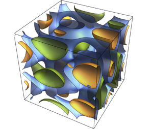
Despite this potential for significantly augmented Lagrangian kinematics and solute mixing and transport dynamics, it has recently been shown (Lester et al. Reference Lester, Dentz, Bandopadhyay and Le Borgne2021) that steady 3-D Darcy flow in heterogeneous porous media with an isotropic hydraulic conductivity field admits highly constrained Lagrangian kinematics, similar to that of steady 2-D flow. These constraints arise as these flows all have vorticity that is everywhere orthogonal to their velocity, leading to zero helicity (an invariant measure of the topological complexity of a flow) across the entire class of isotropic Darcy flows. Lester et al. (Reference Lester, Dentz, Bandopadhyay and Le Borgne2021) show that these helicity-free flows admit a pair of coherent streamfunctions that are topologically planar (although they may be highly convoluted in highly heterogeneous porous media), and the streamlines formed by intersections of the level sets (2-D streamsurfaces) of these streamfunctions are open and topologically equivalent to straight lines. Thus the confinement of streamlines to coherent 2-D streamsurfaces imposes kinematic constraints to steady 3-D isotropic Darcy flow that are very similar to those of steady 2-D flows.
While the study of Lester et al. (Reference Lester, Dentz, Bandopadhyay and Le Borgne2021) generates insights into the Lagrangian kinematics of steady 3-D isotropic Darcy flow, an outstanding question is the quantitative impact of these kinematic constraints upon fluid deformation, which in turn govern mixing, dispersion and transport of diffusive solutes. In this study, we address this question by developing an orthogonal streamfunction coordinate system that inherently enforces the kinematic constraints of these flows. This coordinate system is then used to derive an ab initio coupled continuous time random walk (CTRW) model for fluid deformation that is in essence a 3-D extension of the fluid stretching model derived by Dentz et al. (Reference Dentz, Lester, Le Borgne and de Barros2016b) for 2-D Darcy flow. When compared to general steady 3-D flows, we find that the kinematic constraints associated with steady 3-D isotropic Darcy flow severely retard fluid deformation, and so invite questions as to the suitability of isotropic Darcy flow as a representative model of flow and transport in highly heterogeneous porous media. These quantitative predictions of fluid deformation will be used in future studies to develop predictions of solute mixing and dispersion in isotropic 3-D Darcy flow.
We limit scope to steady 3-D isotropic Darcy flows with smooth and finite hydraulic conductivity fields in the absence of flow sources and sinks (and thus stagnation points) and domain boundaries, as many of these features can violate the helicity-free condition. Although this scenario does not arise commonly in practical applications, it does serve as an important case for understanding these fundamental issues. An important extension to this study is the analysis of the Lagrangian kinematics, mixing and dispersion at the Darcy scale in anisotropic porous media. These flows are not helicity free, and so are not subject to the same kinematic constraints as isotropic Darcy flow and are a subject of ongoing research. While many synthetic porous materials exhibit locally isotropic hydraulic conductivity, the majority of naturally occurring materials such as sedimentary rocks and natural fibres exhibit strongly anisotropic hydraulic conductivity (Bear Reference Bear1972). Despite this, locally isotropic models are often employed in fundamental studies of solute transport and dispersion, and in applied studies when full characterisation of the hydraulic conductivity has not been performed. Hence it is important to understand the implications of using a locally isotropic model of hydraulic conductivity upon solute transport and mixing.
The remainder of this paper is structured as follows. In § 2, we review briefly the kinematics of isotropic Darcy flow from the study of Lester et al. (Reference Lester, Dentz, Bandopadhyay and Le Borgne2021), and in § 3, we use these results to develop a streamfunction coordinate system that automatically imposes the kinematic constraints associated with isotropic Darcy flow. In this section, we address the long-standing question of whether helicity-free flows always give rise to a unique pair of mutually orthogonal streamfunctions, and provide a geometric argument in the affirmative. In § 4, we then use these orthogonal streamfunctions as a basis for a coordinate system to generate closed-form solutions for the components of the fluid deformation gradient tensor. In § 5, we provide a numerical example to illustrate the deformation structure and orthogonality of the streamfunction coordinates for a model isotropic 3-D Darcy flow. An ab initio CTRW framework for the evolution of the deformation tensor in statistically stationary random flows is developed in § 6, and measures of transverse and longitudinal fluid deformation are introduced. Finally, conclusions are made in § 7.
2. The kinematics of 3-D isotropic Darcy flow
2.1. Governing equations and kinematics
To uncover the impact of kinematic constraints imposed by steady 3-D Darcy flow upon diffusive transport and mixing, in this section we briefly review the results of Lester et al. (Reference Lester, Dentz, Bandopadhyay and Le Borgne2021) that the helicity- and stagnation-free nature of these flows admits a dual streamfunction representation. Steady 3-D Darcy flow in a heterogeneous porous medium with a scalar hydraulic conductivity field (henceforth described as isotropic Darcy flow) is described by the Darcy equation
 \begin{equation} \boldsymbol{v}(\boldsymbol{x})={-}(k(\boldsymbol{x})/\theta)\, \boldsymbol{\nabla}\phi(\boldsymbol{x}),\end{equation}
where  $\boldsymbol {x}=(x_1,x_2,x_3)$ denotes physical space in Cartesian coordinates,
  $\boldsymbol {v}(\boldsymbol {x})$ is the fluid velocity,
  $k(\boldsymbol {x})$ is the scalar hydraulic conductivity (which is positive and finite),
  $\theta$ is the porosity (henceforth assumed to be constant), and
  $\phi (\boldsymbol {x})$ is the pressure (or flow potential). As the velocity field
  $\boldsymbol {v}$ is divergence-free, from (2.1) the flow potential
  $\phi$ satisfies the advection–diffusion equation
 \begin{equation} \boldsymbol{\nabla}\boldsymbol{\cdot}\boldsymbol{v}=\nabla^2\phi+\boldsymbol{\nabla} f\boldsymbol{\cdot}\boldsymbol{\nabla}\phi=0,\end{equation}
where  $f\equiv \ln (k/\theta )$. Two key properties of (2.1) significantly constrain the Lagrangian kinematics of isotropic Darcy flow. The first defining characteristic of Darcy flow is that it does not admit stagnation points in the flow (Bear Reference Bear1972) in the absence of sources and sinks, and away from domain boundaries. This constrains the streamline topology, as recirculation regions cannot occur in the flow, so streamlines are open. The second defining characteristic of Darcy flow is that the helicity density
  $h(\boldsymbol {x})$ (defined as the dot product of velocity and vorticity) is everywhere zero (Moffatt Reference Moffatt1969). This is shown by the vector identity
 \begin{equation} h\equiv\boldsymbol{v}\boldsymbol{\cdot} \boldsymbol\omega=(k/\theta)\, \boldsymbol{\nabla}\phi\boldsymbol{\cdot} (\boldsymbol{\nabla}\phi\times\boldsymbol{\nabla} (k/\theta))=0,\end{equation}
where  $\boldsymbol \omega \equiv \boldsymbol {\nabla }\times \boldsymbol {v}=\boldsymbol {\nabla }\phi \times \boldsymbol {\nabla } k$ is the vorticity vector. The volume integral of the helicity density
  $h$ over the flow domain
  $\varOmega$ is defined as total helicity
  $H$ (Moffatt Reference Moffatt1969),
 \begin{equation} H=\int_\varOmega h \, {\rm d}\varOmega, \end{equation}
which is an invariant measure of the topological complexity of the flow. Sposito (Reference Sposito1994, Reference Sposito1997, Reference Sposito2001) recognised that the helicity-free nature of isotropic Darcy flow means that they have simple flow topology, and so proposed that these flows admit a lamellar set of non-intersecting Lamb surfaces (Lamb Reference Lamb1932) throughout the flow domain. These coherent material surfaces are spanned by streamlines and vorticity lines, and so organise streamlines of the flow and impose constraints on the Lagrangian kinematics. These surfaces were then used in Lester et al. (Reference Lester, Dentz, Borgne and Barros2018) as a coordinate basis for a stochastic model of fluid deformation in isotropic 3-D Darcy flow. However, it was determined subsequently (Lester et al. Reference Lester, Bandopadhyay, Dentz and Le Borgne2019) that Lamb surfaces exist only for trivial isotropic 3-D Darcy flows, invalidating this stochastic model.
Subsequently, Lester et al. (Reference Lester, Dentz, Bandopadhyay and Le Borgne2021) established that isotropic Darcy flows admit a pair of coherent 3-D streamfunctions. In this study, we use these streamfunctions as the basis for quantification of fluid deformation in isotropic Darcy flow, and so briefly review the basis for the existence of these streamfunctions as follows. Stagnation-free flows with zero helicity density are recognised to have integrable (Arnol'd Reference Arnol'd1965; Hénon Reference Hénon1966; Holm & Kimura Reference Holm and Kimura1991) particle trajectories, in the dynamical systems sense. This integrability condition (Arnol'd Reference Arnol'd1997) means that the 3-D advection equation
 \begin{equation} \frac{{\rm d}\boldsymbol{v}}{{\rm d}\boldsymbol{x}}= v[\boldsymbol{x}(t,t_0;\boldsymbol{X})],\quad \boldsymbol{x}(t_0,t_0;\boldsymbol{X})=\boldsymbol{X},\end{equation}
for the fluid tracer position  $\boldsymbol {x}(t,t_0;\boldsymbol {X})$ (where
  $\boldsymbol {X}$ gives the Lagrangian coordinates of the initial particle location) admits a pair of conserved quantities (invariants) denoted
  $\psi _1(\boldsymbol {x})$,
  $\psi _2(\boldsymbol {x})$ that may be interpreted as streamfunctions of the flow. Streamsurfaces then arise as level sets of these streamfunctions, and as the flow is stagnation free and helicity free (i.e. it does not possess knotted or closed flow paths), these streamsurfaces are topologically planar. Streamlines of the flow then arise at the intersection of
  $\psi _1$ and
  $\psi _2$ streamsurfaces, so these streamfunctions are constant along a streamline:
 \begin{equation} \psi_1(\boldsymbol{x}(t,t_0;\boldsymbol{X}))=\psi_1(\boldsymbol{X}), \quad \psi_2(\boldsymbol{x}(t,t_0;\boldsymbol{X}))= \psi_2(\boldsymbol{X}).\end{equation}
The invariants ( $\psi _1$,
  $\psi _2$) allow the 3-D advection ordinary differential equation (2.5) to be simplified to the one-dimensional (1-D) definite integral (hence the terminology ‘integrable’)
 \begin{equation} \frac{{\rm d}s}{{\rm d}t}=v(s;\psi_1,\psi_2)\Rightarrow t(s)=\int_0^s \frac{1}{v(s;\psi_1,\psi_2)}\, {\rm d}s,\end{equation}
where  $s$ is the distance travelled by a fluid particle along its trajectory, and
  $v(s;\psi _1,\psi _2)$ is the magnitude of the fluid velocity at distance
  $s$. The integrable nature of 3-D isotropic Darcy flow also means that chaotic advection is not possible in these flows as the braiding of streamlines is not possible, even if the hydraulic conductivity field is strongly heterogeneous.
This is in direct contrast to random pore-scale flows that have been shown (Lester, Trefry & Metcalfe Reference Lester, Trefry and Metcalfe2016a; Lester et al. Reference Lester, Dentz and Le Borgne2016b; Turuban et al. Reference Turuban, Lester, Le Borgne and Méheust2018, Reference Turuban, Lester, Heyman, Le Borgne and Méheust2019; Heyman et al. Reference Heyman, Lester, Turuban, Méheust and Le Borgne2020; Souzy et al. Reference Souzy, Lhuissier, Méheust, Le Borgne and Metzger2020; Heyman, Lester & Le Borgne Reference Heyman, Lester and Le Borgne2021) to be inherently chaotic, even if the porous media is homogeneous at the pore scale. As stated by the Poincaré–Bendixson theorem, only continuous systems with three or more degrees of freedom can admit chaotic dynamics. Consequently, chaotic behaviour (even weakly so) is the norm rather than the exception in random systems with sufficient degrees of freedom. Conversely, the kinematic constraints associated with the helicity-free condition (2.3) in isotropic Darcy flow effectively reduce this three degrees of freedom system (associated with the three spatial dimensions) to a two degrees of freedom system that is not chaotic.
2.2. Streamfunction representation
An inherently divergence-free representation for the velocity field  $\boldsymbol {v}$ is given by the Euler representation
 \begin{equation} \boldsymbol{v}={-}k\,\boldsymbol{\nabla}\phi=\boldsymbol{\nabla}\psi_1\times \boldsymbol{\nabla} \psi_2,\end{equation}
where the fluid velocity  $\boldsymbol {v}$ is orthogonal to the streamfunction gradients
  $\boldsymbol {\nabla } \psi _1$ and
  $\boldsymbol {\nabla } \psi _2$. The stagnation-free condition (
 $\boldsymbol {v}\neq \boldsymbol {0}$) for isotropic Darcy flow ensures that the streamfunctions is single-valued, i.e.
  $\boldsymbol {\nabla } \psi _1\neq \boldsymbol {0}$ and
  $\boldsymbol {\nabla } \psi _2\neq \boldsymbol {0}$. The helicity-free condition (2.3) has been used by several authors (Zijl Reference Zijl1986; Lester et al. Reference Lester, Dentz, Bandopadhyay and Le Borgne2021) to derive the following governing equations for the streamfunctions
  $\psi _1$ and
  $\psi _2$:
 \begin{gather} \nabla^2\psi_1-\boldsymbol{\nabla} f\boldsymbol{\cdot} \boldsymbol{\nabla} \psi_1 =\frac{(\boldsymbol{B}\times\boldsymbol{\nabla} \psi_2)\boldsymbol{\cdot} (\boldsymbol{\nabla} \psi_1\times\boldsymbol{\nabla} \psi_2)}{\|\boldsymbol{\nabla} \psi_1 \times\boldsymbol{\nabla} \psi_2\|}, \end{gather}
 \begin{gather}\nabla^2\psi_2-\boldsymbol{\nabla} f\boldsymbol{\cdot} \boldsymbol{\nabla} \psi_2= \frac{(\boldsymbol{B}\times\boldsymbol{\nabla} \psi_1)\boldsymbol{\cdot} (\boldsymbol{\nabla} \psi_1\times\boldsymbol{\nabla} \psi_2)}{\|\boldsymbol{\nabla} \psi_1\times\boldsymbol{\nabla} \psi_2\|}, \end{gather}
where
 \begin{equation} \boldsymbol{B}\equiv(\boldsymbol{\nabla} \psi_1\boldsymbol{\cdot} \boldsymbol{\nabla} )\boldsymbol{\nabla} \psi_2-(\boldsymbol{\nabla} \psi_2\boldsymbol{\cdot} \boldsymbol{\nabla} )\boldsymbol{\nabla} \psi_1.\end{equation}
Lester et al. (Reference Lester, Dentz, Bandopadhyay and Le Borgne2021) showed that, to within numerical precision, solution of (2.9) and (2.10) yields the same velocity field  $\boldsymbol {v}$ as the solution of (2.2) for Darcy flow. In that study, it was shown that the integrable nature of isotropic Darcy flow implies that fluid deformation is limited to algebraic-in-time deformation, and that streamlines in porous media with statistically stationary hydraulic conductivity cannot converge or diverge without bound, leading to zero macroscopic transverse dispersion in the absence of diffusion. As such, the existence of the streamfunction pair
  $(\psi _1, \psi _2)$ imposes significant constraints on the Lagrangian kinematics of isotropic Darcy flow. In this study, we quantify how these kinematics impact macroscopic mixing, dispersion and transport in the presence of local-scale dispersion. To quantify these impacts, in the next section we introduce a streamfunction coordinate system that automatically imposes the kinematic constraints inherent to heterogeneous isotropic Darcy flow.
3. Streamfunction coordinates
3.1. Uniqueness and orthogonality of streamfunction coordinates
In this section, we introduce a coordinate system for quantification of transport processes in 3-D isotropic Darcy flow. The existence of the streamfunction pair ( $\psi _1$,
  $\psi _2$) generates a natural coordinate system that provides a convenient basis for the study of fluid deformation, mixing and dispersion in steady Darcy flows. Along with the flow potential
  $\phi$, these streamfunctions form the curvilinear coordinate system
  $(\phi,\psi _1,\psi _2)$ that we term streamfunction coordinates. From (2.8), the streamfunction gradients are orthogonal to the potential gradient, but the streamfunction gradients are not mutually orthogonal as in general
  $\boldsymbol {\nabla } \psi _1\boldsymbol {\cdot } \boldsymbol {\nabla } \psi _2 \neq 0$. In Lester et al. (Reference Lester, Dentz, Bandopadhyay and Le Borgne2021), it was shown that non-orthogonality between
  $\boldsymbol {\nabla } \psi _1$ and
  $\boldsymbol {\nabla } \psi _2$ significantly complicates the expression of spatial derivatives in the streamfunction coordinate system
  $(\phi,\psi _1,\psi _2)$ due to the presence off-diagonal terms in the metric tensor. However, the streamfunctions
  $(\psi _1,\psi _2)$ are not unique, as demonstrated (Peymirat & Fontaine Reference Peymirat and Fontaine1999) by the functions
  $\psi _1^\prime (\psi _1,\psi _2)$ and
  $\psi _2^\prime (\psi _1,\psi _2)$, where
 \begin{equation} \boldsymbol{\nabla} \psi_1^\prime\times\boldsymbol{\nabla} \psi_2^\prime= \left(\frac{\partial\psi_1^\prime}{\partial\psi_1}\, \frac{\partial\psi_2^\prime}{\partial\psi_2} -\frac{\partial\psi_2^\prime}{\partial\psi_1}\, \frac{\partial\psi_1^\prime}{\partial\psi_2} \right)(\boldsymbol{\nabla} \psi_1\times\boldsymbol{\nabla} \psi_2), \end{equation}
hence  $\psi _1^\prime$ and
  $\psi _2^\prime$ are also streamfunctions if and only if
 \begin{equation} \frac{\partial\psi_1^\prime}{\partial\psi_1}\, \frac{\partial\psi_2^\prime}{\partial\psi_2} -\frac{\partial\psi_2^\prime}{\partial\psi_1}\, \frac{\partial\psi_1^\prime}{\partial\psi_2}=1.\end{equation}
So there is an infinite set of streamfunctions that satisfy (2.8). The question of whether there exists a pair of mutually orthogonal streamfunctions (where  $\boldsymbol {\nabla } \psi _1^\prime \boldsymbol {\cdot } \boldsymbol {\nabla } \psi _2^\prime =0$) amongst this set has been considered previously in the field of magnetic field topology, where the magnetic field vector
  $\boldsymbol {B}_0$ is represented in terms of the Euler potentials
  $\alpha$ and
  $\beta$ as
  $\boldsymbol {B}_0=\boldsymbol {\nabla } \alpha \times \boldsymbol {\nabla } \beta$. Rankin, Kabin & Marchand (Reference Rankin, Kabin and Marchand2006) show that these potentials, along with the direction of the magnetic field, form an orthogonal coordinate system if and only if there exist no field-aligned magnetic currents. In the context of fluid mechanics, this corresponds to the zero helicity density condition (2.3). Similarly, Hui & Kudriakov (Reference Hui and Kudriakov2001) and Hui & He (Reference Hui and He1997) argue that orthogonal streamline coordinates exist for helicity-free flows but do not provide an explicit proof per se.
Indeed, the general problem regarding the existence of a triply orthogonal system of surfaces (corresponding to the level sets of  $\phi$,
  $\psi _1$ and
  $\psi _2$) has a rich history dating back to the early nineteenth century, and has been addressed by many mathematicians, including Gauss, Lamé, Bonnet, Cayley and Darboux. Weatherburn (Reference Weatherburn1926) shows that the so-called Lamé equations for the existence of triply orthogonal coordinates can be expressed in terms of a second-order differential equation for the unit normal
  $\boldsymbol {n}$ projecting from one family of surfaces. In recent years, several studies have established a direct relationship between specific integrable systems and triply orthogonal coordinates (Terng & Uhlenbeck Reference Terng and Uhlenbeck1998), and there exist strong connections between classes of integrable systems and triply orthogonal coordinates (Zakharov Reference Zakharov1998). Despite these advances, an explicit proof that helicity-free flows yield a triply orthogonal coordinate system is an outstanding problem.
In the following, we provide a geometric argument for the sufficient condition that helicity-free flows admit a pair of orthogonal streamfunctions, and in § 5, we show that this argument is satisfied for a numerically computed steady 3-D Darcy flow. In §§ 3.3 and 2 of the supplementary material (available at https://doi.org/10.1017/jfm.2022.556), we also prove the associated necessary condition that orthogonal streamline coordinates can yield only helicity-free flows. We begin by considering a 2-D isopotential surface  $\mathcal {S}_{\phi ^*}$ that corresponds to
  $\phi =\phi ^*=\text {const}$. Weatherburn (Reference Weatherburn1926) shows that a family of non-intersecting surfaces exists in 3-D space if and only if the unit normal
  $\boldsymbol {n}$ to one of the surfaces satisfies the condition of normality
 \begin{equation} \boldsymbol{n}\boldsymbol{\cdot} (\boldsymbol{\nabla} \times\boldsymbol{n})=0,\end{equation}
where the unit normal vector to  $\mathcal {S}_{\phi ^*}$ is given explicitly as
  $\boldsymbol {n}=\boldsymbol {\nabla } \phi /|\boldsymbol {\nabla } \phi |=\boldsymbol {v}/v$, and so (3.3) is satisfied directly by the helicity-free condition (2.3). Dupin's theorem states that ‘orthogonal coordinate surfaces intersect along lines of principal curvature’, so from the gauge freedom associated with the streamfunction coordinates (3.2), there exist two families of orthogonal curves (denoted respectively
  $(\psi _1^*=\text {const.},\phi ^*)$,
  $(\psi _2^*=\text {const.},\phi ^*)$) that may be identified as streamfunctions that foliate this isosurface via the lines of principal curvature and thus form a local 2-D orthogonal coordinate system on this surface. Thus, although two families of orthogonal curves can be easily constructed that foliate
  $\mathcal {S}_{\phi ^*}$, the question remains as to whether the curves
  $(\psi _1^*,\phi ^*)$,
  $(\psi _2^*,\phi ^*)$ can be extended off
  $\mathcal {S}_{\phi ^*}$ to form the pair of stream surfaces (
 $\psi _1^*$,
  $\psi _2^*$) that are both mutually orthogonal and normal to all other isopotential surfaces
  $\mathcal {S}_{\phi }$.
This persistence of orthogonality of  $\psi _1^*$,
  $\psi _2^*$ corresponds to an angle-preserving transform between the curves
  $(\psi _1^*,\phi ^*)$,
  $(\psi _2^*,\phi ^*)$ on
  $\mathcal {S}_{\phi ^*}$ and the corresponding curves
  $(\psi _1^*,\phi ^{**})$,
  $(\psi _2^*,\phi ^{**})$ on another arbitrary isopotential surface
  $\mathcal {S}_{\phi ^{**}}$ (where
  $\phi ^{**}=\text {const.}$). As the streamsurfaces
  $\psi _1^*$,
  $\psi _2^*$ are invariant (material) surfaces, this angle-preserving (conformal) transform corresponds to irrotational flow (zero vorticity) within each isopotential surface
  $\mathcal {S}_\phi$. Hence the helicity-free condition (2.3) may be interpreted as an angle-preserving transform from one isopotential surface to another (as the flow is irrotational in the plane normal to the flow direction, i.e.
  $\boldsymbol {v}\boldsymbol {\cdot } \boldsymbol \omega =0$). Hence if the streamfunctions
  $\psi _1$,
  $\psi _2$ manifest as orthogonal curves on one isopotential surface, then
  $\psi _1$,
  $\psi _2$ are mutually orthogonal for all isopotential surfaces. This angle-preserving property of helicity-free flows was also identified by Hui & Kudriakov (Reference Hui and Kudriakov2001) and Hui & He (Reference Hui and He1997) in developing the argument that helicity-free flows admit orthogonal streamline coordinates.
In §§ 3.3 and 2 of the supplementary material, we develop the necessary proof that all orthogonal streamline coordinate systems of the form  $(\phi,\psi _1,\psi _2)$, where
 \begin{equation} \boldsymbol{\nabla} \phi_1\boldsymbol{\cdot} \boldsymbol{\nabla} \psi = 0, \quad \boldsymbol{\nabla} \phi_2\boldsymbol{\cdot} \boldsymbol{\nabla} \psi = 0, \quad \boldsymbol{\nabla} \psi_1\boldsymbol{\cdot} \boldsymbol{\nabla} \psi_2 = 0,\end{equation}
render the helicity density to be zero. Whilst this necessary condition does not prove the sufficient condition that helicity-free flows guarantee the existence of an orthogonal streamfunction pair, we then assume the sufficient condition to hold based on the geometric argument above and those of Rankin et al. (Reference Rankin, Kabin and Marchand2006), Hui & Kudriakov (Reference Hui and Kudriakov2001) and Hui & He (Reference Hui and He1997). In § 5, we use a numerical example explicitly to show how a unique pair of orthogonal streamfunction coordinates arises in isotropic 3-D Darcy flow.
As the magnitude of the Darcy velocity  $|\boldsymbol {v}|$ (and the pressure gradient
  $|\boldsymbol {\nabla } \phi |$) must be positive and finite, from (2.8) the magnitude of the streamfunction gradients
  $|\boldsymbol {\nabla } \psi _1|$,
  $|\boldsymbol {\nabla } \psi _2|$ must also be everywhere positive and finite. In conjunction with the orthogonality condition (3.4a–c), this condition means that any point
  $\boldsymbol {x}_0$ in isotropic Darcy flow is defined uniquely by the local values of the fluid pressure and streamfunctions as
  $\boldsymbol \xi _0\equiv (\phi (\boldsymbol {x}_0),\psi _1(\boldsymbol {x}_0), \psi _2(\boldsymbol {x}_0))$. Hence this set of scalar functions represents the orthogonal curvilinear streamfunction coordinate system
 \begin{equation} (\xi^1,\xi^2,\xi^3)\equiv(\phi,\psi_1,\psi_2),\quad \boldsymbol{\nabla} \xi^i\boldsymbol{\cdot} \boldsymbol{\nabla} \xi^j=0\quad \text{for }i\neq j,\end{equation}
which is invertible as the Jacobian  $J\equiv \det [\boldsymbol {J}]$ (where
  $\boldsymbol {J}=\partial \xi ^i/\partial x_j$ is the Jacobian matrix) is everywhere non-zero as
  $|\boldsymbol {\nabla } \phi |\neq 0$,
  $|\boldsymbol {\nabla } \psi _1|\neq 0$,
  $|\boldsymbol {\nabla } \psi _2|\neq 0$ everywhere.
In § 3 of the supplementary material, we use the orthogonality condition (3.4a–c) to simplify the streamfunction governing equations (2.9) and (2.10) to the coupled equations
 \begin{gather} \nabla^2\psi_1-\boldsymbol{\nabla} (f-\ln|\boldsymbol{\nabla} \psi_2|^2)\boldsymbol{\cdot} \boldsymbol{\nabla} \psi_1=0, \end{gather}
 \begin{gather}\nabla^2\psi_2-\boldsymbol{\nabla} (f-\ln|\boldsymbol{\nabla} \psi_1|^2)\boldsymbol{\cdot} \boldsymbol{\nabla} \psi_2=0. \end{gather}
In § 4 of the supplementary material, it is shown that these governing equations enforce mutually orthogonal streamfunctions,  $\boldsymbol {\nabla } \psi _1\boldsymbol {\cdot } \boldsymbol {\nabla } \psi _2=0$.
3.2. Scale factors and basis vectors
This coordinate system forms a convenient basis for studying the kinematics of isotropic Darcy flow as it naturally encodes the kinematic constraints of these flows, as will be shown below. The mapping from Cartesian coordinates  $\boldsymbol {x}\equiv (x_1,x_2,x_3)$ to streamfunction coordinates
  $\boldsymbol \xi \equiv (\xi ^1,\xi ^2,\xi ^3)$ defines the metric tensor
  $g_{\alpha \beta }$, the elements of which determine the scale factors
  $h_\alpha$ of the transformation, such that the differential arc length
  ${\rm d}s$ in the coordinate system
  $(\xi ^1,\xi ^2,\xi ^3)$ is then given by
  ${\rm d}s^2=g_{\alpha \beta }\, {\rm d}\xi ^\alpha \, {\rm d}\xi ^\beta$. As the streamfunction and isopotential surfaces are orthogonal (3.4a–c), the covariant metric tensor is diagonal,
 \begin{equation} g_{\alpha\beta}= \left(\begin{array}{ccc} h_1^2 & 0 & 0 \\ 0 & h_2^2 & 0 \\ 0 & 0 & h_3^2 \end{array} \right),\end{equation}
and the components of the covariant  $g_{\alpha \beta }$ and contravariant
  $g^{\alpha \beta }$ metric tensors are related as
  $g_{\alpha \alpha }^{-1}=g^{\alpha \alpha }$. The scale factors
  $h_\alpha$ of the streamfunction coordinate system are simply the spatial gradients of the fluid pressure
  $\phi$ and streamfunctions
  $\psi _1$,
  $\psi _2$,
 \begin{equation} h_\alpha=\sqrt{\sum_{i}\left(\frac{\partial x_i}{\partial \xi^\alpha}\right)^2}=\frac{1}{|\boldsymbol{\nabla} \xi^\alpha|}, \quad \alpha=1,2,3,\end{equation}
so
 \begin{equation} h_1=\left|\frac{1}{\boldsymbol{\nabla} \phi}\right|=\frac{{\rm d}s}{{\rm d}\phi}, \quad h_2=\left|\frac{1}{\boldsymbol{\nabla} \psi_1}\right|= \frac{{\rm d}r}{{\rm d}\psi_1}, \quad h_3=\left|\frac{1}{\boldsymbol{\nabla} \psi_2}\right|= \frac{{\rm d}q}{{\rm d}\psi_2},\end{equation}
where  $s$,
$s$,  $r$,
$r$,  $q$, respectively, are the distances along a streamline, a vector line normal to a
  $\psi _1$ streamsurface, and that for a
  $\psi _2$ streamsurface. From (2.8), (3.10a–c) and the orthogonality condition (3.4a–c), these scale factors are related to the velocity and hydraulic conductivity
  $k$ as
  $1/(h_2h_3)=|\boldsymbol {\nabla } \psi _1|\,|\boldsymbol {\nabla } \psi _2|=v$,
  $h_1/(h_2h_3)=|\boldsymbol {\nabla } \psi _1|\,|\boldsymbol {\nabla } \psi _2|/|\boldsymbol {\nabla } \phi |=k$. Using (2.1) and (3.9), the scale factors
  $h_\alpha$ can be expressed without loss of generality as
 \begin{equation} h_1=\frac{k}{v}, \quad h_2=\sqrt{\frac{m}{v}}, \quad h_3=\frac{1}{\sqrt{m v}}, \end{equation}
where  $m\equiv |\boldsymbol {\nabla } \psi _2|/|\boldsymbol {\nabla } \psi _1|$ is an arbitrary scalar function that quantifies the relative local spacing of the
  $\psi _1$ and
  $\psi _2$ streamsurfaces. In the streamfunction coordinate system, the covariant basis vectors
  $\boldsymbol {g}_\alpha$ are then
 \begin{equation} \boldsymbol{g}_\alpha=\left(\frac{\partial x_1}{\partial \xi^\alpha},\frac{\partial x_2}{\partial\xi^\alpha},\frac{\partial x_3}{\partial\xi^\alpha}\right),\quad \alpha=1,2,3,\end{equation}
which are related to the unit covariant basis vectors  $\hat {\boldsymbol {g}}_i$ and contravariant vectors
  $\boldsymbol {g}^i$ via the scale factors
  $h_\alpha$ as
 \begin{equation} \hat{\boldsymbol{g}}_\alpha=\frac{1}{h_\alpha}\,\boldsymbol{g}_\alpha =h_\alpha\boldsymbol{g}^\alpha.\end{equation}
An arbitrary vector  $\boldsymbol {a}$ may be represented in terms of these basis vectors as
  $\boldsymbol {a}=a^i\boldsymbol {g}_i=a^{\langle i\rangle }\hat {\boldsymbol {g}}_i=a_i\boldsymbol {g}^i$, with
  $a^{\langle i\rangle }=h_i a^i=a_i/h_i$. The Jacobian
  $J$ of the transform between Cartesian and streamfunction coordinates is then related to the determinant of the covariant metric tensor as
  $J=\sqrt {\det {g_{\alpha \beta }}}=h_1h_2h_3=k/v^2$, and so is spatially variable. In § 1 of the supplementary material, we use the above results to derive the divergence, gradient and curl operators in the streamfunction coordinate system.
3.3. Orthogonality of streamfunction coordinates
This orthogonal coordinate system automatically recovers the helicity-free condition as the velocity field is given as
 \begin{equation} \boldsymbol{v}=\boldsymbol{\nabla} \psi_1\times\boldsymbol{\nabla} \psi_2=\frac{1}{h_2h_3}\, \hat{\boldsymbol{g}}_2\otimes\hat{\boldsymbol{g}}_3=v\hat{\boldsymbol{g}}_1, \end{equation}
where  $v=|\boldsymbol {v}|$, and from § 1 of the supplementary material, the vorticity is then
 \begin{equation} \boldsymbol\omega=\boldsymbol{\nabla} \times\boldsymbol{v}=\frac{1}{h_1h_2h_3} \left\{\frac{\partial(v h_1)}{\partial\psi_2}\,h_2\hat{\boldsymbol{g}}_2- \frac{\partial(v h_1)}{\partial\psi_1}\,h_3\hat{\boldsymbol{g}}_3\right\}. \end{equation}
Hence the helicity  $h=\boldsymbol \omega \boldsymbol {\cdot } \boldsymbol {v}$ is zero as the basis vectors
  $\hat {\boldsymbol {g}}_i$ are mutually orthogonal. As such, only helicity-free flows admit a pair of streamfunctions that are mutually orthogonal, and hence an orthogonal streamfunction coordinate system.
4. Fluid deformation in isotropic Darcy flow
4.1. Fluid deformation in Cartesian coordinates
As fluid mixing and dispersion arise from the interplay of diffusion and fluid deformation, in this section we develop expressions for the deformation of fluid elements in isotropic Darcy flow. The streamfunction coordinate system developed in § 2 forms a convenient basis for investigation of deformation of fluid elements in isotropic Darcy flow as the kinematic constraints associated with these flows are imposed automatically by the coordinate system. For simplicity of exposition, we first consider the deformation of fluid elements in the Cartesian coordinate system  $\boldsymbol {x}$ before extending this to the streamfunction coordinates
  $\boldsymbol \xi$, which as will be shown, presents significant simplification for the computation of fluid deformation. Such deformation is quantified by the fluid deformation gradient tensor
  $\boldsymbol {F}(\boldsymbol {X},t)$, which quantifies how the infinitesimal vector
  ${\rm d}\boldsymbol {x}(t;\boldsymbol {X})$ in the Eulerian frame deforms from its reference state
  ${\rm d} \boldsymbol {X}(t = 0;\boldsymbol {X}) = {\rm d}\boldsymbol {X}$ in the Lagrangian frame as
 \begin{equation} {\rm d}\boldsymbol{x}=\boldsymbol{F}(\boldsymbol{X},t)\boldsymbol{\cdot} {\rm d}\boldsymbol{X}, \end{equation}
and equivalently,
 \begin{equation} F_{ij} \equiv\frac{\partial x_i(t;\boldsymbol{X})}{\partial X_j}, \quad \boldsymbol{F}(\boldsymbol{X},t)=\frac{\partial x_i(t; \boldsymbol{X})}{\partial X_j}\,\boldsymbol{e}_i\otimes \boldsymbol{e}^j ,\end{equation}
where  $\hat {\boldsymbol {e}}_i=\boldsymbol {e}_i=\boldsymbol {e}^i$ respectively are the
  $i$th unit, covariant and contravariant vectors (which are all equal) in the Cartesian coordinate system. If we consider
  $\boldsymbol \varPhi _t(\boldsymbol {X})$ as the flow (in the dynamical systems sense of Arnol'd Reference Arnol'd1997) that maps the initial position
  $\boldsymbol {X}$ of a fluid particle at time
  $t=0$ to its current position
  $\boldsymbol {x}$ at time
  $t$, then this flow is given as a solution of the advection equation (2.5), such that
  $\boldsymbol {x}(t,0,\boldsymbol {X})=\boldsymbol \varPhi _t(\boldsymbol {X})$ and so
  $\boldsymbol {X}=\boldsymbol \varPhi _{t=0}(\boldsymbol {X})$. From this definition, the deformation gradient tensor may also be defined by the derivative of the flow with respect to the Lagrangian coordinate as
 \begin{equation} \boldsymbol{F}(\boldsymbol{X},t)=\frac{\partial \varPhi^i_t(\boldsymbol{X})}{\partial X^j}\,\boldsymbol{e}_i \otimes\boldsymbol{e}^j.\end{equation}
Following this definition, the deformation gradient tensor  $\boldsymbol {F}(t)$ evolves with travel time
  $t$ along a Lagrangian trajectory (streamline) as
 \begin{equation} \frac{{\rm d}\boldsymbol{F}(\boldsymbol{X},t)}{{\rm d}t}= \boldsymbol\epsilon(t)\boldsymbol{\cdot} \boldsymbol{F}(\boldsymbol{X},t), \quad \boldsymbol{F}(\boldsymbol{X},0)=\boldsymbol{1},\end{equation}
where  $\boldsymbol \epsilon (t)$ is the transpose of the velocity gradient tensor:
 \begin{equation} \boldsymbol\epsilon(t)\equiv\boldsymbol{\nabla} \boldsymbol{v}(\boldsymbol{x}(t; \boldsymbol{X}))^{\rm T}=\epsilon_{ij}(t)\,\boldsymbol{e}_i\otimes \boldsymbol{e}^j.\end{equation}
4.2. Fluid deformation in streamfunction coordinates
Solution of the deformation gradient evolution equation (4.4) is simplified greatly in the streamfunction coordinates, where we denote the Eulerian frame via the streamfunction coordinates  $\boldsymbol \xi =\{\xi ^1,\xi ^2,\xi ^3\}$, and the corresponding Lagrangian frame in the streamfunction coordinates,
  $\boldsymbol \varXi =\{\varXi ^1,\varXi ^2,\varXi ^3\}$ (where
  $\boldsymbol \xi =\boldsymbol \varXi$ at
  $t=0$). The corresponding flow in streamfunction coordinates is then denoted as
  $\boldsymbol \xi =\boldsymbol \chi _t(\boldsymbol \varXi )$ (where
  $\boldsymbol \varXi =\boldsymbol \chi _{t=0}(\boldsymbol \varXi )$), so the various frames are related as
 \begin{equation} \begin{array}{ccccc} & \varXi^i & \xrightarrow{{\large \xi^i=\chi^i_t(\varXi^j)}} & \xi^i & \\ \varXi^i(X^j) & \Bigg\uparrow & & \Bigg\downarrow & x^i(\xi^j)\\ & X^i & \xrightarrow{{\large x^i=\varPhi^i_t(X^j)}} & x^i & \end{array}, \end{equation}
where the top and bottom rows, respectively, represent the streamfunction and Cartesian frames, and the left and right columns, respectively, represent the reference and current frames. In the streamfunction coordinate frame, the streamfunction deformation tensor  $\boldsymbol {F}(\boldsymbol \varXi,t)$ relates the differential reference vector
  ${\rm d}\boldsymbol \varXi$ to its current configuration
  ${\rm d}\boldsymbol \xi$ as
 \begin{equation} \boldsymbol{F}(\boldsymbol\varXi,t)=\frac{\partial \xi_i(t;\boldsymbol\varXi)}{\partial \varXi_j}\,\boldsymbol{g}_i \otimes\boldsymbol{G}^j , \end{equation}
where  $\boldsymbol {G}^j$ is the
  $j$th contravariant vector of the streamfunction coordinate system in the Lagrangian frame (i.e. at
  $t=0$). This deformation tensor may also be expressed in terms of the corresponding flow
  $\boldsymbol \xi =\boldsymbol \chi _t(\boldsymbol \varXi )$ in streamfunction coordinates as
 \begin{equation} \boldsymbol{F}(\boldsymbol\varXi,t)=\frac{\partial\chi^i_t (\boldsymbol\varXi)}{\partial\varXi^j}\,\boldsymbol{g}_i\otimes \boldsymbol{G}^j.\end{equation}
To render the components of the streamfunction deformation tensor physically meaningful, we express it in terms of the physical components  $\hat {F}_{ij}(\boldsymbol \varXi,t)$ as
 \begin{equation} \boldsymbol{F}(\boldsymbol\varXi,t)=\frac{\partial\chi^i_t (\boldsymbol\varXi)}{\partial\varXi^j}\,\frac{h_i}{H_j}\, \hat{\boldsymbol{g}}_i\otimes\hat{\boldsymbol{G}}^j\equiv \hat{F}_{ij}(\boldsymbol\varXi,t)\,\hat{\boldsymbol{g}}_i \otimes\hat{\boldsymbol{G}},\end{equation}
where  $\hat {\boldsymbol {g}}_i$,
  $\hat {\boldsymbol {G}}_j$ are the respective unit vectors in the current and reference frames, and the corresponding scale factors are
  $h_i$,
  $H_j$. Following Marsden & Hughes (Reference Marsden and Hughes1994), the streamfunction deformation gradient tensor can be translated into the Cartesian frame as
 \begin{align} \boldsymbol{F}(\boldsymbol\varXi,t) &=\frac{\partial\chi^i_t(\boldsymbol\varXi)}{\partial\varXi^j}\, \boldsymbol{g}_i\otimes\boldsymbol{G}^j=\frac{\partial x^m}{\partial\xi^i}\, \frac{\partial\chi^i_t(\boldsymbol\varXi)}{\partial\varXi^j}\, \frac{\partial \varXi^j}{\partial X^n}\, \boldsymbol{e}_m\otimes\boldsymbol{e}^n\nonumber\\ &=J_{mi}^{{-}1}(t)\,\frac{\partial\chi^i_t(\boldsymbol\varXi)}{\partial\varXi^j}\, J_{kn}(0)\,\boldsymbol{e}_m\otimes\boldsymbol{e}^n =\frac{\partial\varPhi^i_t(\boldsymbol{X})}{\partial X^j}\, \boldsymbol{e}_m\otimes\boldsymbol{e}^n =\boldsymbol{F}(\boldsymbol{X},t), \end{align}
where  $J_{ij}(t)$ is the
  $ij$th element of the Jacobian matrix at position
  $\boldsymbol {x}(t;\boldsymbol {X})$. Hence, as expected, the deformation gradient tensor is frame-indifferent. However, the elements of the physical deformation tensor transform between the Cartesian and streamfunction frames as
 \begin{equation} F_{mn}(\boldsymbol{X},t)=h_i\,J_{mi}^{{-}1}(t)\,\hat{F}_{ij} (\boldsymbol\varXi,t)\,H_J^{{-}1}\,J_{jn}(0)=\hat{J}_{mi}^{{-}1}(t)\, \hat{F}_{ij}(\boldsymbol\varXi,t)\,\hat{J}_{jn}(0),\end{equation}
where  $\hat {J}_{ij}(t)=\nabla _i\xi _j/h_j$ represents the normalised Jacobian matrix that transforms physical vector components from the Cartesian to the streamfunction frame:
 \begin{equation} {\rm d}\boldsymbol\xi={\rm d}\hat{\xi}_i\,\hat{\boldsymbol{g}}_i, \quad {\rm d}\hat{\xi}_i=\hat{J}_{ij}x_j. \end{equation}
As  $\det [\hat {J}_{ij}(t)]=1$ and
  $\hat {J}_{ij}(t)\,\hat {J}_{ji}(t)=\delta _{ij}$, the normalised Jacobian represents a proper orthogonal transform that takes the form of a rotation matrix between the physical Cartesian and streamfunction frames. Correspondingly, differential vector elements in the four physical frames are then related as
 \begin{equation} \begin{array}{ccccc} & {\rm d}\hat{\varXi}^i & \xrightarrow {{\rm d}\hat\xi^i=\hat{F}_{ij}(\boldsymbol\varXi,t) \, {\rm d}\hat\varXi^j} & {\rm d}\hat\xi^i & \\ {\rm d}\varXi^i=\hat{J}_{ij}(0)\, {\rm d}X^j & \Bigg\uparrow & & \Bigg\downarrow & {{\rm d} x}^i=\hat{J}_{ij}(t)^{{-}1} \, {\rm d}\hat\xi^j\\ & {\rm d}X^i & \xrightarrow{{{\rm d} x}^i=F_{ij}(\boldsymbol{X}, t) \, {\rm d}X^j} & {{\rm d} x}^i & \end{array}. \end{equation}
Using (4.11), elements of the Cartesian deformation tensor can be determined by transforming the corresponding elements of the streamfunction deformation tensor via the Jacobian matrix in the reference and current frames. As indicated above, mapping of the differential element  ${\rm d}\boldsymbol {X}$ to
  ${\rm d}\boldsymbol {x}$ is equivalent to first transforming
  ${\rm d}\boldsymbol {X}$ to
  ${\rm d}\boldsymbol \varXi$ via the Jacobian matrix at
  $t=0$, then using the streamfunction deformation tensor to map to
  ${\rm d}\boldsymbol \varXi$, and finally mapping back to
  ${\rm d}\boldsymbol {x}$ via the inverse of the Jacobian matrix at
  $t=t$. Although this approach appears to be somewhat convoluted, the major advantage is that the Jacobian matrix is known everywhere and the deformation tensor
  $\boldsymbol {F}$ has an analytic solution in streamfunction coordinates, as will become clear in the following.
4.3. Solution of fluid deformation in streamfunction coordinates
Following (4.4), the physical components of the streamfunction deformation tensor evolve with time according to
 \begin{equation} \frac{{\rm d}\boldsymbol{F}(\boldsymbol\varXi,t)}{{\rm d}t}= \boldsymbol\epsilon(t)\boldsymbol{\cdot} \boldsymbol{F}(\boldsymbol\varXi,t)\, \frac{{\rm d}\hat{F}_{ij}(\boldsymbol\varXi,t)}{{\rm d}t}= \hat\epsilon_{ij}(t)\,\hat{F}_{ij}(\boldsymbol\varXi,t),\quad \hat{F}_{ij}(\boldsymbol\varXi,0)=\delta_{ij},\end{equation}
where  $\boldsymbol \epsilon (t)$ is the velocity gradient tensor in streamfunction coordinates:
  $\boldsymbol \epsilon (t)=\epsilon _{ij}(t)\,\boldsymbol {g}_i\otimes$
  $\boldsymbol {g}^j= \hat {\epsilon }_{ij}(t)\,\hat {\boldsymbol {g}}_i\otimes \hat {\boldsymbol {g}}^j$, where
  $\hat {\epsilon }_{ij}(t)=h_i/h_j\,\epsilon _{ij}(t)$. From (1.12) in the supplementary material, the gradient of a contravariant vector
  $\boldsymbol {v}$ may be expressed in terms of the Christoffel symbols
  $\varGamma ^i_{jk}$ (Aris Reference Aris1956; Nguyen-Schfer & Schmidt Reference Nguyen-Schfer and Schmidt2014) as
 \begin{equation} \boldsymbol{\nabla} \boldsymbol{v}=\boldsymbol{\nabla} (v^i\boldsymbol{g}_i)= \left(\frac{\partial v^i}{\partial\xi^j}+v^j\varGamma^k_{ij}\right) \boldsymbol{g}_i\otimes\boldsymbol{g}^j=\frac{h_i}{h_j} \left(\frac{\partial v^i}{\partial\xi^j}+v^j\varGamma^k_{ij}\right) \hat{\boldsymbol{g}}_i\otimes\hat{\boldsymbol{g}}^j,\end{equation}
and from (1.1) in the supplementary material, the fluid velocity  $\boldsymbol {v}$ in streamfunction coordinates simplifies to
 \begin{align} \boldsymbol{v}(\phi,\psi_1,\psi_2)&=k\,\boldsymbol{\nabla} \phi= \frac{k}{h_1}\,\hat{\boldsymbol{g}}_1=v\hat{\boldsymbol{g}}_1,\nonumber\\ &=\boldsymbol{\nabla} \psi_1\times\boldsymbol{\nabla} \psi_2=\frac{1}{h_2}\,\hat{\boldsymbol{g}}_2 \times\frac{1}{h_3}\,\hat{\boldsymbol{g}}_3=\frac{1}{h_2h_3}\, \hat{\boldsymbol{g}}_1=v\hat{\boldsymbol{g}}_1. \end{align}
In § 5 of the supplementary material, (4.15) and (4.16) are used to derive the streamfunction velocity gradient tensor, which has non-zero physical components
 \begin{gather} \hat{\epsilon}_{11}(t)=\frac{\partial v}{\partial s}, \quad \hat{\epsilon}_{22}(t)={-}\frac{1}{2}\,\frac{\partial v}{\partial s}+ \frac{v}{2}\,\frac{\partial\ln m}{\partial s}, \quad \hat{\epsilon}_{33}(t)={-}\frac{1}{2}\,\frac{\partial v}{\partial s}- \frac{v}{2}\,\frac{\partial\ln m}{\partial s}, \end{gather}
 \begin{gather}\hat{\epsilon}_{12}(t)=2\dot\gamma_r-\omega_r\equiv\sigma_r, \quad \hat{\epsilon}_{13}(t)=2\dot\gamma_q-\omega_q \equiv\sigma_q, \end{gather}
where  $\dot \gamma$ and
  $\omega$ represent shear deformation and vorticity:
 \begin{equation} \dot\gamma_\alpha\equiv\frac{\partial v}{\partial\alpha}, \quad \omega_\alpha\equiv v\,\frac{\partial\ln k}{\partial\alpha}, \quad \alpha=r,q. \end{equation}
In streamfunction coordinates, the velocity gradient  $\boldsymbol \epsilon (t)$ has a simple upper triangular structure
 \begin{equation} \boldsymbol\epsilon(t)=\left( \begin{array}{ccc} \hat\epsilon_{11}(t) & \hat\epsilon_{12}(t) & \hat\epsilon_{13}(t) \\ 0 & \hat\epsilon_{22}(t) & 0 \\ 0 & 0 & \hat\epsilon_{33}(t) \end{array} \right),\end{equation}
where the diagonal components  $\epsilon _{ii}(t)$ (with
  $\sum _i\epsilon _{ii}=0$ due to incompressibility) correspond to normal fluid strains due to changes in velocity
  $v$ and lateral expansion/contraction (as quantified by
  $m$) with distance
  $s$ along a streamline. Conversely, the non-zero off-diagonal components
  $\sigma _1$,
  $\sigma _2$ are associated with shear
  $\dot \gamma _\alpha$ and vorticity
  $\omega _\alpha$ (with
  $\alpha =r,q$) within the
  $\psi _1$ and
  $\psi _2$ streamsurfaces. Note that
  $\hat \epsilon _{23}=0$ due to the helicity-free nature of the flow, hence there is no fluid shear in the direction orthogonal to the flow direction, and fluid deformation is decoupled between the
  $(1,2)$ and
  $(1,3)$ surfaces. As such, 3-D isotropic Darcy flow behaves as two superposed 2-D flows, and the kinematics of these flows is overwhelmingly 2-D in nature. We will show that this restriction has significant implications for fluid deformation, dispersion and mixing.
Several studies (Dentz et al. Reference Dentz, Lester, Le Borgne and de Barros2016b; Adachi Reference Adachi1986; Winter Reference Winter1982) have shown that steady 2-D flows also admit an upper triangular velocity gradient tensor in streamline coordinates. Lester et al. (Reference Lester, Dentz, Borgne and Barros2018) also show that steady 3-D helicity-free flows have an upper triangular velocity gradient tensor in an orthogonal coordinate system comprised of velocity  $\boldsymbol {v}$, vorticity
  $\boldsymbol \omega$ and the Lamb vector
  $\boldsymbol \ell \equiv \boldsymbol {v}\times \boldsymbol \omega$. However, it was shown subsequently (Lester et al. Reference Lester, Bandopadhyay, Dentz and Le Borgne2019) that the Lamb surfaces associated with the Lamb vector (where Lamb surfaces are level sets of the scalar potential field
  $\mathcal {H}$, and
  $\boldsymbol \ell =\boldsymbol {\nabla } \mathcal {H}$) proposed by Sposito (Reference Sposito1997, Reference Sposito2001) do not exist for general steady 3-D helicity-free flows, so the orthogonal vectors
  $(\boldsymbol {v},\boldsymbol \omega,\boldsymbol \ell )$ do not form a holonomic (coordinate) basis, and thus a coherent coordinate system. Hence (4.20) is the first valid exposition that the velocity gradient tensor in 3-D isotropic Darcy flow (and indeed all helicity-free flows) is upper triangular and the coupling component
  $\hat {\epsilon }_{23}$ is zero.
The upper triangular structure of the velocity gradient tensor in (4.20) admits a particularly simple solution for the fluid deformation equation (4.4), in that the deformation gradient tensor is also upper triangular:
 \begin{equation} \boldsymbol{F}(\boldsymbol\varXi,t)=\left( \begin{array}{ccc} \hat{F}_{11} & \hat{F}_{12} & \hat{F}_{13} \\ 0 & \hat{F}_{22} & 0 \\ 0 & 0 & \hat{F}_{33} \end{array} \right),\end{equation}
with  $\det \boldsymbol {F}(\boldsymbol \varXi,t)=\prod _i \hat {F}_{ii}(\boldsymbol \varXi,t)=1$ due to incompressibility. The diagonal components of
  $\boldsymbol {F}(\boldsymbol \varXi,t)$ are given by (4.4) as
 \begin{equation} \hat{F}_{ii}(\boldsymbol\varXi,t)=\exp\left[\int_0^t {\rm d} t^\prime \epsilon_{ii}(t^\prime)\right],\quad i=1,2,3, \end{equation}
which can be solved explicitly via the change of variable  ${\rm d}t={\rm d}s/v$ to yield
 \begin{align} \hat{F}_{11}(\boldsymbol\varXi,t) =\frac{v(t)}{v(0)}, \quad \hat{F}_{22}(\boldsymbol\varXi,t)=\sqrt{\frac{v(0)}{v(t)}\, \frac{m(t)}{m(0)}}, \quad \hat{F}_{33}(\boldsymbol\varXi,t) =\sqrt{\frac{v(0)}{v(t)}\, \frac{m(0)}{m(t)}},\end{align}
where  $v(t)=|\boldsymbol {v}(\boldsymbol \xi (t;\boldsymbol \varXi ))|$ and
  $m(t)=m(\boldsymbol \xi (t;\boldsymbol \varXi ))$. In statistically stationary and isotropic media,
  $v(t)$ and
  $m(t)$ fluctuate in a random and uncorrelated manner, hence the principal strains
  $F_{ii}$ also fluctuate around a unit mean value due to local fluctuations in the fluid velocity field. As such, the ensemble average for the principal strains are all unity,
 \begin{equation} \langle \hat{F}_{ii}(\boldsymbol\varXi,t)\rangle = 1,\quad i=1,2,3,\end{equation}
which is also reflected by the fact that all zero helicity density flows are non-chaotic (Arnol'd Reference Arnol'd1965), hence the infinite-time Lyapunov exponent is identically zero:
 \begin{equation} \lambda=\langle\ln \hat{F}_{22}(\boldsymbol\varXi,t) \rangle={-} \langle\ln \hat{F}_{33}(\boldsymbol\varXi,t) \rangle=0. \end{equation}
In contrast, the magnitude of the non-zero shear strains  $\hat {F}_{12}$,
  $\hat {F}_{13}$ grow without bound as
 \begin{gather} \hat{F}_{12}(\boldsymbol\varXi,t)=v(t)\int_0^t {\rm d}t^\prime\, \frac{\epsilon_{12}(t^\prime)\,\hat{F}_{22}(\boldsymbol\varXi, t^\prime)}{v(t^\prime)}=v(t)\,\sqrt{\frac{v(0)}{m(0)}}\int_0^t {\rm d}t^\prime\,\frac{\sigma_r(t^\prime)\, \sqrt{m(t^\prime)}}{v(t^\prime)^{3/2}}, \end{gather}
 \begin{gather}\hat{F}_{13}(\boldsymbol\varXi,t)=v(t)\int_0^t {\rm d}t^\prime\, \frac{\epsilon_{13}(t^\prime)\,\hat{F}_{33}(\boldsymbol\varXi, t^\prime)}{v(t^\prime)}=v(t)\,\sqrt{v(0)\,m(0)}\int_0^t {\rm d} t^\prime\,\frac{\sigma_q(t^\prime)}{v(t^\prime)^{3/2} \sqrt{m(t^\prime)}}, \end{gather}
where the shear rates are  $\sigma _r(t)=\sigma _r(\boldsymbol \xi (t;\boldsymbol \varXi ))$ and
  $\sigma _q(t)=\sigma _q(\boldsymbol \xi (t;\boldsymbol \varXi ))$. As particle advection along a streamline is governed by the advection equation (2.5), these integrals may be reformulated according to
  ${\rm d}t={\rm d}s/v(s)$, where
  $s$ is the distance along a streamline, leading to the spatial integrals
 \begin{gather} \hat{F}_{12}(s)=v(s)\,\sqrt{\frac{v(0)}{m(0)}}\int_0^s {\rm d} s^\prime\, \frac{\sigma_r(s^\prime)\,\sqrt{m(s^\prime)}}{v(s^\prime)^{5/2}}, \end{gather}
 \begin{gather}\hat{F}_{13}(s)=v(s)\,\sqrt{v(0)\,m(0)}\int_0^s {\rm d} s^\prime\, \frac{\sigma_q(s^\prime)}{v(s^\prime)^{5/2}\sqrt{m(s^\prime)}}. \end{gather}
Thus persistent fluid deformation in 3-D isotropic Darcy flows is due solely to the fluid shears  $\sigma _r(s)$,
  $\sigma _q(s)$ that are oriented in the orthogonal
  $(1,2)$ and
  $(1,3)$ surfaces that are both parallel to the streamwise direction. An expression similar to (4.28) has been derived by Dentz et al. (Reference Dentz, Lester, Le Borgne and de Barros2016b) for the deformation of material elements in 2-D steady heterogeneous flow in streamline coordinates. In the case of 2-D steady flow considered by Dentz et al. (Reference Dentz, Lester, Le Borgne and de Barros2016b), the stretching factor
  $m(s)$ in (4.28) is omitted, and the denominator of the integral contains a factor
  $v^3$ rather than
  $v^{5/2}$. Note that fluid deformation in
  $(1,3)$ surfaces of 3-D isotropic Darcy flow (given by (4.29)) is very similar to that of
  $(1,2)$ deformation (given by (4.28)), with the only differences that
  $m(t)\mapsto 1/m(t)$ and
  $\sigma _r(t)\mapsto \sigma _q(t)$. Hence the extension from steady 2-D flow to steady isotropic 3-D Darcy flow involves additional shear deformation in the
  $(1,3)$-plane (which is absent in 2-D), and a scaling factor
  $\sqrt {m(t)/m(0)}$ that reflects the fact that whilst the overall flow is volume-preserving, the
  $(1,2)$ and
  $(1,3)$ surfaces themselves are not necessarily area-preserving.
In random stationary 2-D flows, the shear rate  $\sigma (s)$ has been shown (Dentz et al. Reference Dentz, Lester, Le Borgne and de Barros2016b) to fluctuate around a mean value of zero, whilst the inverse velocity magnitude
  $1/v$ (which corresponds to the waiting time distribution in a finite region of the flow) often follows a heavy-tailed distribution for heterogeneous porous media. Dentz et al. (Reference Dentz, Lester, Le Borgne and de Barros2016b) show that for 2-D steady random flows, the correlation between fluid shear (
 $\sigma )$ and velocity (as
  $1/v^3$) processes leads to persistent elongation of material elements despite the zero mean nature of the shear rate
  $\sigma$. For 2-D steady flows, the factors driving this
  $1/v^3=(1/v)(1/v)(1/v)$ velocity dependence are as follows: (i) one factor
  $1/v$ arises from the increased residence time of fluid elements in low-velocity regions; (ii) a second factor
  $1/v$ arises from the compression of fluid elements in the streamwise direction while shear is being applied; and (iii) the third factor
  $1/v$ is associated with the divergence of streamlines in low-velocity regions. Hence episodes of low velocity (where the velocity can become vanishingly small) in 2-D steady random flows can lead to a significant amplification of shear deformation and persistent elongation of material elements in the streamwise direction.
The same basic mechanisms are at play in 3-D isotropic Darcy flow, with the exception that the third factor above has a different scaling,  $1/v^{5/2}=(1/v)(1/v)(1/v^{1/2})$, where the third factor associated with streamline divergence in low-velocity regions has changed from
  $1/v$ to
  $1/v^{1/2}$ due to the introduction of the third spatial dimension. In the case of 3-D isotropic Darcy flow, there exist pairs of 2-D streamfunctions that diverge with changes in the local velocity (rather than divergence of 1-D streamlines in steady 2-D flow), as reflected by the scaling
  $|\boldsymbol {\nabla } \psi _1|\,|\boldsymbol {\nabla } \psi _2|=v$ in (3.10a–c), so each set of streamsurfaces diverges with respect to
  $v$ as
  $1/v^{1/2}$. Quantitative differences in the divergence of each set of streamsurfaces is quantified by the scalar function
  $m=|\boldsymbol {\nabla } \psi _2|/|\boldsymbol {\nabla } \psi _1|$ introduced in (3.10a–c). Thus, rather than
  $1/v$ for the third factor above for 2-D flows, the divergence of streamsurfaces leads to a factor
  $\sqrt {m/v}$,
  $1/(\sqrt {mv})$, respectively in the integrals of (4.28), (4.29). Similar to the 2-D case, for random stationary flows, the longitudinal shears
  $\sigma _r$,
  $\sigma _q$ have zero mean (as the ensemble-averaged or spatially averaged flow is a translation flow with zero shear), and both the scale factor
  $m$ and the fluid velocity
  $v$ fluctuate in a stationary manner. However, the net result of the interactions above is that for 3-D isotropic Darcy flow, fluid stretching due to the shears
  $\sigma _r$,
  $\sigma _q$ is amplified nonlinearly in low-velocity regions (by the term
  $v^{5/2}$ in (4.28), (4.29)), leading to persistent growth of material elements.
5. Fluid deformation and streamline structure: numerical example
These dynamics and the structure of isotropic Darcy flow are illustrated in figure 1, which depicts isotropic Darcy flow in a triply periodic unit cube (3-torus)  $\mathbb {T}^3: \boldsymbol {x}\equiv (x_1,x_2,x_ 3)=[0,1]\times [0,1]\times [0,1]$, with the spatially periodic hydraulic log-conductivity field
 \begin{align} f(\boldsymbol{x})&=2.3 \sin(2 \pi (x_1 + 0.34)) \sin(4 \pi (x_2 - 0.14))\nonumber\\ &\quad + 0.9 \sin(2 \pi (x_1 - 0.26)) \sin(2 \pi (x_3 + 0.44))\nonumber\\ &\quad - 1.5 \sin(4 \pi (x_3 - 0.86)) \sin(2 \pi (x_3 - 0.24)), \end{align}
shown in figure 1(a). Darcy flow in this porous medium is driven by the unit mean potential gradient  $\bar {\phi }(\boldsymbol {x})=-x_1$, and the potential fluctuation
  $\tilde \phi (\boldsymbol {x})$ that results from spatial heterogeneity of the hydraulic log-conductivity field
  $f(\boldsymbol {x})$ (where
  $\phi (\boldsymbol {x})=\bar {\phi }(\boldsymbol {x})+\tilde {\phi }(\boldsymbol {x})$) is given by the Darcy equation (2.2) as
 \begin{equation} \nabla^2\tilde\phi+\boldsymbol{\nabla} f\boldsymbol{\cdot} \boldsymbol{\nabla} \tilde\phi= \frac{\partial f}{\partial x_1},\end{equation}
subject to periodic boundary conditions on  $\mathbb {T}^3$. Equation (5.2) is solved on a regular
  $256^3$ finite difference grid (corresponding to a resolution of 64 grid points per correlation length of
  $f(\boldsymbol {x})$) via an iterative Krylov sparse method to precision
  $10^{-16}$, and the corresponding potential field
  $\phi (\boldsymbol {x})$ is shown in figure 1(b). This grid resolution is required to generate a high-precision continuous potential field
  $\phi (\boldsymbol {x})$ via cubic interpolation from the grid values, and the velocity field is then given by (2.1). The corresponding relative divergence error
  $d(\boldsymbol {x})\equiv \boldsymbol {\nabla } \boldsymbol {\cdot } \boldsymbol {v}/\|\boldsymbol {\nabla } \boldsymbol {v}\|$ from a sample of
  $10^5$ random points in the domain is found to have average error 0.05 %, and the helicity is identically zero.

Figure 1. Isosurfaces of (a) the log-conductivity field  $f(\boldsymbol {x})$ and (b) isopotential
  $\phi (\boldsymbol {x})$ surfaces for 3-D isotropic Darcy flow in a triply periodic unit cube. The streamline and deformation structure of this flow is shown in (c), where the reference streamline (black) is shadowed by two neighbouring streamlines that are offset in the
  $\psi _1$ (red) and
  $\psi _2$ (blue) directions. Note that the scale transverse to the black streamline has been amplified by a factor of
  $10^6$ to aid visualisation, and the area of the ellipses scales inversely with fluid velocity
  $\boldsymbol {v}$. The black ellipses depict transverse fluid deformation at different time intervals from the reference state (circle) at the start (leftmost end) of the streamlines, and the principal axes of these ellipses (which define the
  $\psi _1$ and
  $\psi _2$ coordinate directions) are given by the deformation tensor components
  $\hat {F}_{22}(t)$,
  $\hat {F}_{33}(t)$. As shown, the red and blue streamlines always coincide with the principal axes of the deformation ellipses, thus maintaining orthogonality of the streamline coordinates throughout the flow domain. The green line in (c) depicts the evolution of a material line of length
  $l_r(t)$ that is initially oriented in the
  $\psi _1$ direction.
Although this flow is solved numerically in terms of the flow potential  $\phi$ rather than the orthogonal streamfunctions
  $\psi _1$,
  $\psi _2$, the orthogonal structure of these streamfunctions can be visualised via the deformation structure of the flow. Equation (4.21) shows that in streamfunction coordinates, projection of the fluid deformation tensor
  $\boldsymbol {F}(\boldsymbol \varXi,t)$ onto an isopotential surface normal to the flow simply involves principal stretches in the
  $\psi _1$,
  $\psi _2$ directions,
 \begin{equation} \boldsymbol{F}_{2\text{-D}}(\boldsymbol\varXi,t)=\left( \begin{array}{cc} \hat{F}_{22} & 0 \\ 0 & \hat{F}_{33} \end{array} \right),\end{equation}
as the helicity-free condition precludes transverse shear (as quantified by  $\hat {F}_{23}$,
  $\hat {F}_{32}$). These principal stretches can be used to identify the unique orthogonal streamfunction coordinates in the computed Darcy flow. By computing the Cartesian deformation tensor
  $\boldsymbol {F}(\boldsymbol {X},t)$ along a Lagrangian trajectory (reference streamline) of the flow shown as the black line in figure 1(c), this deformation tensor can be rotated to align with the velocity vector, and the projection into the 2-D isosurface is taken (see § 6 of the supplementary material for details). The principal axes
  $\boldsymbol {d}_r(t)$,
  $\boldsymbol {d}_q(t)$ associated with the resultant 2-D transverse deformation tensor then identify the coordinate directions
  $\psi _1$,
  $\psi _2$, and are related to the streamfunction deformation tensor components as
 \begin{equation} \hat{F}_{22}(t)=\frac{|\boldsymbol{d}_r(t)|}{|\boldsymbol{d}_r(0)|}, \quad \hat{F}_{33}(t)= \frac{|\boldsymbol{d}_q(t)|}{|\boldsymbol{d}_q(0)|}, \end{equation}
As shown in figure 1(c), these principal axes  $\boldsymbol {d}_r(t)$,
  $\boldsymbol {d}_q(t)$ coincide with (red, blue) streamlines of the flow that are seeded at a distance of
  $\delta =10^{-6}$ from the reference streamline (black) in the
  $\psi _1$,
  $\psi _2$ directions. As the principal axes
  $\boldsymbol {d}_r(t)$,
  $\boldsymbol {d}_q(t)$ of the deformation ellipse are always orthogonal, orthogonality of the streamfunctions
  $\psi _1$,
  $\psi _2$ arises throughout the flow domain.
Figure 1 shows clearly the basis for the existence and persistence of mutually orthogonal streamfunctions in zero helicity flows. Here, the deformation transverse to the flow direction consists of only fluid stretching and/or contraction via the principal axes, so these principal axes form a continuous 2-D orthogonal coordinate system over an isopotential surface normal to the flow. The absence of rotation associated with vortical motion in these isopotential surfaces means that this 2-D orthogonal coordinate system then extends in the streamwise direction, thus forming a continuous 3-D orthogonal coordinate system that consists of the two families of streamsurfaces and the isopotential surfaces of the flow. However, unlike the case for non-orthogonal streamfunctions (Lester et al. Reference Lester, Dentz, Bandopadhyay and Le Borgne2021; Zijl Reference Zijl1986), presently there is no known set of partial differential equations to generate these orthogonal streamfunctions. The non-orthogonal streamfunctions (obtained by solution of (2.9), (2.10)) of a similar Darcy flow are shown in Figure 5(b) of (Lester et al. Reference Lester, Dentz, Bandopadhyay and Le Borgne2021), and the associated orthogonal streamfunctions are expected to have a similar structure. Fortunately, many of the theoretical results derived in this study in orthogonal streamfunction coordinates can be translated into the Cartesian frame and so can be used to understand and quantify the deformation structure of these flows.
Figures 2(a)–2(c) show the distribution of velocity magnitude  $v(t)$, shear rates
  $\sigma _r(t)$,
  $\sigma _q(t)$, and relative streamfunction gradients
 \begin{align} \frac{|\boldsymbol{\nabla} \psi_1(0)|}{|\boldsymbol{\nabla} \psi_1(t)|} =\sqrt{\frac{v(0)\,m(t)}{v(t)\,m(0)}}=\frac{1}{\delta}\,|\boldsymbol{d}_r(t)|, \quad \frac{|\boldsymbol{\nabla} \psi_2(0)|}{|\boldsymbol{\nabla} \psi_2(t)|}= \sqrt{\frac{v(0)\,m(0)}{v(t)\,m(t)}}=\frac{1}{\delta}\,|\boldsymbol{d}_q(t)|, \end{align}
along the reference streamline shown in figure 1(c). Figure 2(d) shows the evolution of the lengths  $l_r(t)$ and
  $l_q(t)$ of two material lines of initial length
  $\delta =10^{-6}$ and respective orientation in the the
  $\psi _1$ and
  $\psi _2$ directions. As shown in figure 1(c), the lengths of these material lines evolve with changes in the streamline spacing (as quantified by
  $\hat {F}_{22}$,
  $\hat {F}_{33}$) and shear parallel to the streamwise direction (as quantified by
  $\hat {F}_{12}$,
  $\hat {F}_{13}$), and so are given explicitly as
 \begin{gather} l_r(t)=|\boldsymbol{F}(\boldsymbol{X},t)\boldsymbol{\cdot} \boldsymbol{d}_r(t)|=\delta\sqrt{\hat{F}_{12}(t)^2 +\hat{F}_{22}(t)^2}, \end{gather}
 \begin{gather}l_q(t)=|\boldsymbol{F}(\boldsymbol{X},t)\boldsymbol{\cdot} \boldsymbol{d}_q(t)|=\delta\sqrt{\hat{F}_{13}(t)^2+ \hat{F}_{33}(t)^2}, \end{gather}
where the initial persistent growth of  $l_r(t)$ and
  $l_q(t)$ arises through
  $\hat {F}_{12}$,
  $\hat {F}_{13}$. Figure 2 shows clearly how fluid velocity, shear and streamline spacing control the growth of material lines as described by (4.26), (4.27). For example, the rapid growth of
  $l_r(t)$ and
  $l_q(t)$ over the time period
  $t\in [2,3]$ corresponds to the low-velocity region in figure 2(a), and the growth of
  $l_r(t)$ is more pronounced than that of
  $l_q(t)$ due to the larger streamfunction spacing in figure 2(c). Conversely, the low-velocity region in figure 2(a) over the period
  $t\in [6,8]$ does not significantly alter
  $l_r(t)$ and
  $l_q(t)$ as the corresponding shear rates in figure 2(b) are both small. Figure 2(d) shows that the calculation of
  $l_r(t)$ and
  $l_q(t)$ agrees via: (i) computation of the Cartesian deformation tensor
  $\boldsymbol {F}(\boldsymbol {X},t)$; (ii) computation of
  $\hat {F}_{12}(t)$,
  $\hat {F}_{13}(t)$, respectively, in (4.26), (4.27); and (iii) numerical calculation via particle tracking. Hence this agreement validates derivation of the evolution of the deformation gradient tensor in streamfunction coordinates in § 4. Note that although the flow field in this example is not random (due to the deterministic nature of the hydraulic conductivity field in (5.1)), the fluid velocity, shear rate and elongations along streamlines exhibit intermittent behaviour similar to that observed for steady random 3-D flows (Lester et al. Reference Lester, Dentz, Borgne and Barros2018). For such random flows, intermittency of fluid velocity, shear rate and material deformation is due to the persistence of the flow velocity over the correlation scale of the hydraulic conductivity field and decorrelation over longer length scales. Such observations form the basis for a stochastic model of fluid deformation in random isotropic 3-D Darcy flow that will be developed in the next section.
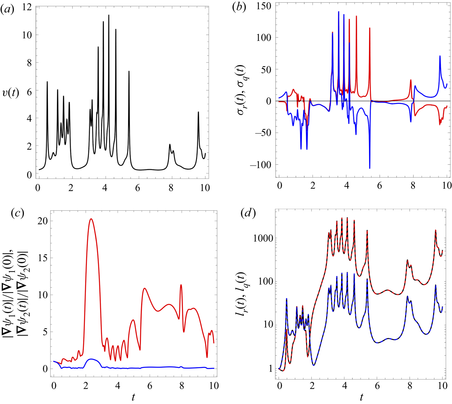
Figure 2. (a–c) Distributions along the black streamline shown in figure 1(c). (a) Distribution of velocity magnitude  $v(t)$. (b) Distributions of shear rates: red line,
  $\sigma _r(t)$; blue line,
  $\sigma _q(t)$. (c) Distributions of streamfunction gradients: red line,
  $|\boldsymbol {\nabla } \psi _1(t)|/|\boldsymbol {\nabla } \psi _1(0)|$; blue line,
 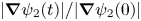 $|\boldsymbol {\nabla } \psi _2(t)|/|\boldsymbol {\nabla } \psi _2(0)|$. (d) Evolution of the relative length
  $l(t)/l(0)$ of a differential line element oriented initially along the
  $\psi _1$ (red dashed line) and
  $\psi _2$ (blue dashed line) coordinates computed from (5.6), (5.7). These relative lengths very closely match those computed from both direct particle tracking (black lines) and the Cartesian deformation tensor (not shown, indistinguishable).
6. Fluid deformation as a continuous time random walk
For steady 3-D isotropic Darcy flow with a random stationary hydraulic conductivity field, the evolution of fluid velocity may be placed in a CTRW framework (Berkowitz et al. Reference Berkowitz, Cortis, Dentz and Scher2006). As fluid deformation is driven by the velocity gradient  $\boldsymbol {\nabla } \boldsymbol {v}$ along streamlines, these processes may also be described by a CTRW process. In this section, we use the CTRW framework to develop closed-form predictions of fluid deformation in heterogeneous isotropic Darcy flow from the deformation evolution equations (4.28) and (4.29). At both the pore and Darcy scales, it is well established that the fluid velocity along a streamline in heterogeneous porous media follows a spatial Markov process (Le Borgne, Dentz & Carrera Reference Le Borgne, Dentz and Carrera2008a,Reference Le Borgne, Dentz and Carrerab; De Anna et al. Reference De Anna, Le Borgne, Dentz, Tartakovsky, Bolster and Davy2013; Edery et al. Reference Edery, Guadagnini, Scher and Berkowitz2014; Kang et al. Reference Kang, Dentz, Le Borgne and Juanes2011; Hakoun, Comolli & Dentz Reference Hakoun, Comolli and Dentz2019; Comolli, Hakoun & Dentz Reference Comolli, Hakoun and Dentz2019). Coarse-graining particle motion on the order of the streamwise correlation length
  $\ell$, the advection equation (2.5) may be described by the CTRW
 \begin{equation} s_{n+1}=s_n+\ell, \quad t_{n+1}=t_n+\frac{\ell}{v_n} \equiv t_n+\tau_n,\end{equation}
where  $s_n$ is the spatial distance along a streamline at time
  $t_n$,
  $v_n$ is the corresponding fluid velocity, and
  $\ell$ is the correlation length of the hydraulic conductivity field. Due to statistical stationarity of the conductivity field and Markovianity of the velocity distribution over distance
  $\ell$, the velocities
  $v_n \equiv v(s_n)$ are identical independently distributed random variables distributed according to the probability density function (PDF)
  $p_v(v)$, which is related to the Eulerian velocity PDF
  $p_e(v)$ as
 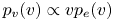 $p_v(v) \propto v p_e(v)$ (Dentz et al. Reference Dentz, Kang, Comolli, Le Borgne and Lester2016a). For strongly heterogeneous media, the Eulerian velocity distribution shows algebraic behaviour for small velocities (Hakoun et al. Reference Hakoun, Comolli and Dentz2019; Comolli et al. Reference Comolli, Hakoun and Dentz2019). This implies that the PDF
  $\psi (t)$ of the temporal increment
  $\tau _n$ in (6.1a,b) is broadly distributed as
 \begin{equation} \psi(t)=\frac{\ell}{t^2}\,p_v\left(\frac{\ell}{t}\right).\end{equation}
6.1. Deformation evolution as a coupled continuous-time random walk
The coarse-grained equations of motion (6.1a,b) of a particle in the CTRW framework can also be used to coarse-grain the deformation evolution equations (4.28) and (4.29), resulting in
 \begin{equation} \hat{F}_{12}(s_n)\equiv\hat{F}_{12,n}=v_n\sqrt{v_0 m_0}\,I_{12,n}, \quad \hat{F}_{13}(s_n)\equiv\hat{F}_{13,n}=v_n\sqrt{\frac{v_0}{m_0}}\, I_{13,n}, \end{equation}
where the coarse-grained integrals  $I_{12,n}$ and
  $I_{13,n}$ in (4.28) and (4.29) are approximated as
 \begin{gather} I_{12,n}\approx\sum_{i=1}^n\rho_{r,n}\ell, \quad \rho_{r,n}\equiv\frac{\sigma_{r,n}}{\sigma_c} \left(\frac{v_c}{v_n}\right)^{5/2}\sqrt{\frac{m_n}{m_c}}, \end{gather}
 \begin{gather}I_{13,n}\approx\sum_{i=1}^n\rho_{q,n}\ell, \quad \rho_{q,n}\equiv \frac{\sigma_{q,n}}{\sigma_c}\left(\frac{v_c}{v_n}\right)^{5/2} \sqrt{\frac{m_c}{m_n}}. \end{gather}
Thus  $I_{12,n}$ and
  $I_{13,n}$ satisfy the recursion relations
 \begin{gather} I_{12,n+1}=I_{12,n}+\rho_{r,n}\ell, \quad t_{n+1}=t_n+\frac{\ell}{v_n}=t_n+\tau_n, \end{gather}
 \begin{gather}I_{13,n+1}=I_{13,n}+\rho_{q,n}\ell, \quad t_{n+1}=t_n+\frac{\ell}{v_n}=t_n+\tau_n, \end{gather}
where the subscripts  $c$ and
  $n$ on
  $v$,
$v$,  $\sigma$,
  $m$ respectively denote characteristic values of these variables and their values at position
  $s_n$. Equations (6.6a,b) and (6.7a,b) are coupled CTRWs in the sense that the process increments
  $\rho _{r,n}$ and
  $\rho _{q,n}$ and the time increments
  $\tau _n$ are fully coupled via the local velocity
  $v_n$. Dentz et al. (Reference Dentz, Lester, Le Borgne and de Barros2016b) assume that for steady 2-D flows, the absolute value of the shear rate
  $\sigma _n$ is correlated strongly with the velocity magnitude
  $v_n$. For statistically isotropic Darcy flow,
  $\sigma _r$ and
  $\sigma _q$ have the same probability distribution. Indeed, for the model Darcy flow considered in § 5,
  $\sigma _r$ and
  $\sigma _q$ have the same distribution, and figure 3(a) indicates that both
  $|\sigma _r|$ and
  $|\sigma _q|$ are correlated strongly with the square of the velocity magnitude as
 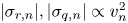 $|\sigma _{r,n}|, |\sigma _{q,n}|\propto v_n^2$. In general, the shear rate may be correlated with the velocity magnitude as
 \begin{equation} |\sigma_{i,n}|=\zeta_n\sigma_c\left(\frac{v_n}{v_c}\right)^{\hat{\alpha}}, \quad i=(r,q),\end{equation}
where  $\hat {\alpha }\approx 2, 1$ for 3-D and 2-D flows, respectively, and
  $\zeta _n$ is a random variable equal to
  $\pm 1$ with equal probability. Equation (6.8) is a general power-law correlation between the local shear rate
  $\sigma _{i,n}$ and velocity
  $v_n$. Several studies (Dentz et al. Reference Dentz, Lester, Le Borgne and de Barros2016b; Lester et al. Reference Lester, Dentz, Borgne and Barros2018) have found such a correlation to hold for steady random 2-D and 3-D flows. For statistically isotropic Darcy flows, the logarithm of the streamfunction relative gradient
  $\ln m_n$ is distributed symmetrically about
  $\ln m=0$, so in conjunction with the equivalence of the distribution of
  $|\sigma _{r}|$ and
  $|\sigma _{q}|$, the increments
  $\rho _r$,
  $\rho _q$ and thus the integrals
  $I_{12}$,
  $I_{13}$ respectively have the same distributions. Indeed, figure 3(b) shows that for the model Darcy flow in § 5, the logarithm of the streamfunction relative gradient
  $\ln m_n$ follows a normal distribution with zero mean and variance
  $\sigma _{\ln m}^2=6.533$ and is found to be uncorrelated to velocity or shear rate. From (6.8), (6.4a,b) and (6.5a,b), the process increments
  $\rho _{i,n}$ in the coupled CTRWs (6.6a,b) and (6.7a,b) are related to the transition times
  $\tau _n=\ell /v_n$ as
 \begin{equation} \rho_{i,n}=\zeta_n\left(\frac{\tau_n}{\tau_v}\right)^\alpha,\quad \alpha=\frac{5}{2}-\hat{\alpha},\quad i=(r,q),\end{equation}
where  $\tau _v\equiv \ell /v_c$,
  $\langle \rho \rangle =0$ and
  $|\rho _{i,n}|=(\tau _n/\tau _v)^\alpha$. In contrast to (6.9), for 2-D flows the index for the elongation increments is related to
  $\hat {\alpha }$ as
  $\alpha =3-\hat {\alpha }$ (Dentz et al. Reference Dentz, Lester, Le Borgne and de Barros2016b), reflecting the stronger coupling between low-velocity regions and fluid deformation in these flows. The joint PDF
  $\psi (\rho,\tau )$ of the process increments and transition times is then
 \begin{equation} \psi(\rho,\tau)=\frac{1}{2}\,\delta\left[|\rho |-\left(\frac{\tau}{\tau_v} \right)^\alpha\right]\psi(\tau).\end{equation}
Thus the index  $\alpha$ can differ significantly between 2-D and 3-D flows: for 2-D flow, Dentz et al. (Reference Dentz, Lester, Le Borgne and de Barros2016b) finds
  $\alpha =3-\hat {\alpha }=2$, whereas for steady 3-D Darcy flow,
  $\alpha =5/2-\hat {\alpha }$. For the specific Darcy flow considered in § 5, it is observed in figure 3(a) that
  $\hat \alpha =2$, hence
  $\alpha =5/2-\hat {\alpha }=1/2$, but different values of
  $\alpha$ are possible for other steady isotropic 3-D Darcy flows. These differences in
  $\alpha$ can result in qualitative differences in the deformation behaviour in these flows. Many porous media flows, including heterogeneous Darcy flow (Hakoun et al. Reference Hakoun, Comolli and Dentz2019), are characterised by a power-law velocity distribution
  $p_v(v)\propto (v/v_c)^{\beta -1}$ for velocities smaller than a characteristic velocity
  $v_c$, where
  $\beta$ decreases with increasing heterogeneity of the hydraulic conductivity field. The corresponding transition time PDF scales as
  $\psi (\tau )\propto (\tau /\tau _v)^{-1-\beta }$ for
  $\tau >\tau _v$. Under these conditions, the CTRWs (6.6a,b) and (6.7a,b) describe a coupled Lévy walk (Dentz et al. Reference Dentz, Le Borgne, Lester and de Barros2015) for each of the deformation tensor components
  $\hat {F}_{12}$,
  $\hat {F}_{13}$ that is parametrised by
  $\alpha$ and
  $\beta$.

Figure 3. (a) Correlation between absolute shear rate  $|\sigma (t)|$ and velocity
  $v(t)$, showing
  $\hat \alpha =2$. (b) Distribution of relative streamfunction gradient
  $m(t)=|\boldsymbol {\nabla } \psi _1|/|\boldsymbol {\nabla } \psi _2|$ for the model 3-D Darcy flow considered in § 5.
The dynamics of this class of coupled Lévy walk has been considered previously in detail by Dentz et al. (Reference Dentz, Le Borgne, Lester and de Barros2015), so these results can be applied directly to the CTRWs (6.6a,b) and (6.7a,b). Dentz et al. (Reference Dentz, Le Borgne, Lester and de Barros2015) derive a range of algebraic scaling behaviours for the moments of  $I_{n}$ that depend upon the parameters
  $\alpha$ and
  $\beta$, which have also been used by Dentz et al. (Reference Dentz, Lester, Le Borgne and de Barros2016b) to quantify fluid deformation in steady 2-D flow. For the case of fluid deformation in steady isotropic 3-D Darcy flow, the results from Dentz et al. (Reference Dentz, Le Borgne, Lester and de Barros2015) indicate that for
  $\alpha \geqslant 1$, the growth of the absolute value of the deformation components
  $\langle |\hat {F}_{1i}(t)|\rangle$ ranges from diffusive (
 $\langle |\hat {F}_{1i}(t)|\rangle \sim t^{1/2}$) to superlinear (
 $\langle |\hat {F}_{1i}(t)|\rangle \sim t^{1+\alpha -\beta }$) growth depending upon the relative magnitudes of
  $\alpha$ and
  $\beta$. For cases where
  $\alpha <1$, Dentz et al. (Reference Dentz, Le Borgne, Lester and de Barros2015) show that growth of the deformation components ranges from diffusive for
  $\beta >2\alpha$ to dispersive for
  $1<\beta <2\alpha$ to weakly anomalous for
  $0<\beta <1$, where the deformation components evolve as
  $\langle |\hat {F}_{1i}(t)|\rangle \sim t^r$, with
 \begin{equation} r=\begin{cases} \alpha, & 0<\beta<1,\\[2pt] \frac{1}{2}+\alpha-\frac{\beta}{2}, & 1<\beta<2\alpha,\\[2pt] \frac{1}{2}, & 2\alpha<\beta. \end{cases}\end{equation}
These scalings are tested by comparison with numerical evaluation of the CTRWs (6.4a,b), (6.5a,b) for various values of  $\alpha$ and
  $\beta$, and the results are shown in figure 4. As expected, (6.11) recovers the correct scaling behaviour of the absolute values of the integrals
  $|I_{12}|$,
  $|I_{13}|$ at long times, and the PDFs of
  $|I_{12}|$,
  $|I_{13}|$ at
  $t=10^3$ are well described by a half-normal distribution. Thus fluid deformation in random stationary 3-D isotropic Darcy flows can admit a diverse range of behaviour ranging from diffusive to superlinear growth, depending upon the correlation between fluid shear and velocity (as characterised by
  $\alpha$) and scaling of the velocity PDF in the small velocity regime (as characterised by
  $\beta$). This coupling leads to algebraic growth of the transverse deformation components as
 \begin{equation} \langle |\hat{F}_{12}(t)|\rangle\sim t^{r_2}, \quad \langle |\hat{F}_{13}(t)|\rangle\sim t^{r_3},\end{equation}
where the power-law indices  $0< r_2$,
  $r_3 < 2$ exhibit different scaling regimes (quantified by (Dentz et al. Reference Dentz, Le Borgne, Lester and de Barros2015)) that depend upon the specific values of
  $\alpha$ and
  $\beta$. It is useful to note that
  $\alpha$ appears to vary minimally from one medium to the next, whereas
  $\beta$ decreases with increasing medium heterogeneity (Dentz et al. Reference Dentz, Lester, Le Borgne and de Barros2016b), hence it may be possible to approximate these parameters from field studies. Although there exist minor differences in values of these exponents for 2-D and 3-D isotropic Darcy flows, the basic mechanism of persistent deformation in 3-D Darcy flows is remarkably similar to that of 2-D flow, where intermittency of low-velocity regions can amplify fluid stretching nonlinearly due to shear oriented parallel to the streamwise direction. The power-law growth of
  $\hat {F}_{12}(t)$ and
  $\hat {F}_{13}(t)$ in (6.12a,b) is consistent with the theory (Arnol'd Reference Arnol'd1965; Ottino Reference Ottino1989) that all non-chaotic helicity-free steady flows involve fluid deformation that scales algebraically in time. The novelty of the CTRW framework is that it quantifies the scaling laws for fluid deformation, and facilitates identification of the mechanisms that govern the various scaling regimes.

Figure 4. (a) Evolution of integrals  $\langle | I(t)|\rangle =\langle | I_{12}(t)|\rangle =\langle | I_{13}(t)|\rangle$ from numerical solution of the CTRWs (6.6a,b), (6.7a,b) (solid lines) and comparison with scalings given by (6.11) (dashed lines) for various values of
  $\alpha$ and
  $\beta$. (b) PDF of
  $| I(t)|$ (points) and fitted half-normal distribution (lines) from numerical solution of (6.6a,b), (6.7a,b) for various values of
  $\alpha$ and
  $\beta$ at
  $t=10^3$.
6.2. Longitudinal and transverse deformation
To illustrate how the deformation tensor controls longitudinal and transverse deformation of fluid elements, we decompose  $\boldsymbol {F}(\boldsymbol \varXi,t)$ into longitudinal and transverse components, respectively, as
  $\boldsymbol {F}(\boldsymbol \varXi,t)=\boldsymbol {F}_l(\boldsymbol \varXi,t)+\boldsymbol {F}_t(\boldsymbol \varXi,t)$, where
 \begin{gather} \boldsymbol{F}_l(\boldsymbol\varXi,t)\equiv\text{diag} (\hat{\boldsymbol{g}}_1)\boldsymbol{\cdot} \boldsymbol{F}(\boldsymbol\varXi,t)= \left( \begin{array}{ccc} \hat{F}_{11} & \hat{F}_{12} & \hat{F}_{13} \\ 0 & 0 & 0 \\ 0 & 0 & 0 \\ \end{array} \right), \end{gather}
 \begin{gather}\boldsymbol{F}_t(\boldsymbol\varXi,t)\equiv\text{diag}(\hat{\boldsymbol{g}}_2+\hat{\boldsymbol{g}}_3)\boldsymbol{\cdot} \boldsymbol{F}(\boldsymbol\varXi,t)= \left( \begin{array}{ccc} 0 & 0 & 0 \\ 0 & \hat{F}_{22} & 0 \\ 0 & 0 & \hat{F}_{33} \\ \end{array} \right), \end{gather}
where  $\text {diag}(\boldsymbol {a})$ is a diagonal matrix comprised of the vector
  $\boldsymbol {a}$ along the diagonal. From (4.1), a differential line element
  $\delta \boldsymbol {l}(\boldsymbol \varXi,t)$ at Lagrangian position
  $\boldsymbol \varXi$ at time
  $t=0$ evolves with time as
 \begin{align} \delta\boldsymbol{l}(\boldsymbol\varXi,t)&=\boldsymbol{F} (\boldsymbol\varXi,t)\boldsymbol{\cdot} \delta\boldsymbol{l}(\boldsymbol\varXi,0) =\boldsymbol{F}_l(\boldsymbol\varXi,t)\boldsymbol{\cdot} \delta\boldsymbol{l} (\boldsymbol\varXi,0)+\boldsymbol{F}_t(\boldsymbol\varXi,t)\boldsymbol{\cdot} \delta\boldsymbol{l}(\boldsymbol\varXi,0)\nonumber\\ &\equiv\delta\boldsymbol{l}_l(\boldsymbol\varXi,t)+ \delta\boldsymbol{l}_t(\boldsymbol\varXi,t), \end{align}
and so may be decomposed into its longitudinal  $\delta \boldsymbol {l}_l(\boldsymbol \varXi,t)$ and transverse
  $\delta \boldsymbol {l}_t(\boldsymbol \varXi,t)$ components. Similarly, the length
  $\delta l(t)$ of these line elements can also be decomposed as
  $\delta l(t)^2=\delta l_l(t)^2+\delta l_t(t)^2$ via
 \begin{align} \delta l(t)&\equiv|\delta\boldsymbol{l}(\boldsymbol\varXi,t)| =\sqrt{\delta\boldsymbol{l}(\boldsymbol\varXi,0)\boldsymbol{\cdot} (\boldsymbol{F}_l^{\rm T}(\boldsymbol\varXi,t)\boldsymbol{\cdot} \boldsymbol{F}_l (\boldsymbol\varXi,t)+\boldsymbol{F}_t^{\rm T}(\boldsymbol\varXi,t)\boldsymbol{\cdot} \boldsymbol{F}_t(\boldsymbol\varXi,t))\boldsymbol{\cdot} \delta\boldsymbol{l} (\boldsymbol\varXi,0)}\nonumber\\ &\equiv\sqrt{\delta l_l(t)^2+\delta l_t(t)^2}. \end{align}
From (6.15), we characterise longitudinal and transverse fluid deformation respectively in terms of the metrics  $\varLambda _l(t)$,
  $\varLambda _t(t)$ as
 \begin{gather} \varLambda_l(t)\equiv\left\langle\frac{\delta l_l(t)}{\delta l_l(0)} \right\rangle=\langle\|\boldsymbol{F}_l(\boldsymbol\varXi,t)\|\rangle= \langle\sqrt{\hat{F}_{11}(\boldsymbol\varXi,t)^2+\hat{F}_{12} (\boldsymbol\varXi,t)^2+\hat{F}_{13}(\boldsymbol\varXi,t)^2}\rangle, \end{gather}
 \begin{gather}\varLambda_t(t)\equiv\left\langle\frac{\delta l_t(t)}{\delta l_t(0)} \right\rangle=\langle\|\boldsymbol{F}_t(\boldsymbol\varXi,t)\|\rangle= \langle\sqrt{\hat{F}_{22}(\boldsymbol\varXi,t)^2+\hat{F}_{33} (\boldsymbol\varXi,t)^2}\rangle, \end{gather}
where  $\varLambda _l(t)$ characterises the longitudinal stretching of fluid elements along streamlines due to shear and vorticity, whereas
  $\varLambda _t(t)$ characterises the transverse deformation due to the separation of streamlines. In Lester et al. (Reference Lester, Dentz, Borgne and Barros2018), we show that the growth rates of these differential deformation metrics are important for different applications. For the pulsed injection of a tracer, growth of the longitudinal metric
  $\varLambda _l(t)$ governs longitudinal mixing and dispersion of the resultant solute plume. For steady 2-D Darcy flow, the mean and variance of the growth of
  $\varLambda _l(t)$ act as inputs (along with the Péclet number
  $Pe$) for predictive models (Le Borgne et al. Reference Le Borgne, Dentz and Villermaux2013, Reference Le Borgne, Dentz and Villermaux2015) of mixing and dispersion in 2-D Darcy flow. Conversely, for continuous injection of a tracer, the growth rate of the transverse element
  $\varLambda _t(t)$ characterises the transverse mixing and dispersion of the plume. Along with the Péclet number
  $Pe$, the mean and variance of the growth rate of
  $\varLambda _t(t)$ are used by Lester et al. (Reference Lester, Dentz and Le Borgne2016b) to predict mixing of a continuously injected source in steady 3-D pore-scale flow. From (4.24) and (6.12a,b), we find that for 3-D steady isotropic Darcy flow, the longitudinal deformation of fluid elements can grow algebraically, whereas the transverse deformation of fluid elements is zero:
 \begin{equation} \varLambda_l(t)\sim t^r, \quad \varLambda_t(t)\sim 1.\end{equation}
In conjunction with molecular diffusion, these deformation rates control the dispersion and mixing of solutes and colloids in isotropic Darcy flow.
7. Conclusions
We have considered the impacts of the Lagrangian kinematics of steady 3-D isotropic Darcy flow upon fluid deformation in isotropic heterogeneous porous media. These flows are characterised by the fact that they are helicity free in that the velocity is everywhere orthogonal to the vorticity, which severely constrains their kinematics. These flows admit a pair of coherent streamfunctions. The intersection of their corresponding streamsurfaces forms highly constrained streamlines that cannot be knotted or braided. Furthermore, as pairs of streamlines cannot diverge, there is zero transverse macro-dispersion. This behaviour arises as streamlines of isotropic Darcy flow are confined to coherent 2-D streamsurfaces that are topologically planar, hence many of the kinematic constraints of 2-D steady flows apply to steady isotropic 3-D Darcy flow. To quantify the impact of these kinematic constraints upon fluid deformation, solute mixing and dispersion, we have used the properties of isotropic Darcy flows to develop an orthogonal coordinate system (comprised of the two streamfunctions and fluid pressure) that imposes automatically the kinematic constraints of these flows. We use this coordinate system to solve the fluid deformation evolution equations in 3-D isotropic Darcy flow, and find that it is remarkably similar to 2-D Darcy flow in that fluid elements do not persistently deform transversely (consistent with zero transverse macro-dispersion), and deform longitudinally only due to shear flow parallel to the flow direction. We develop a coupled continuous time random walk (CTRW) framework to describe the evolution of fluid deformation in the streamfunction coordinates, and show how the structure of these flows controls this process. We introduce measures of ensemble-averaged longitudinal ( $\varLambda _l(t)$) and transverse (
 $\varLambda _t(t)$) fluid deformation, and show that although transverse deformation is zero
  $(\varLambda _l(t)\sim 1)$, longitudinal deformation grows algebraically at a rate that can range from sub-diffusive to ballistic (
 $\varLambda _l(t)\sim t^r$,
  $r\in [0,2]$), and the various scalings match direct numerical calculations of the stretching CTRW. Similar to steady 2-D flow (Dentz et al. Reference Dentz, Lester, Le Borgne and de Barros2016b), the stretching index
  $r$ is controlled by intermittency of the fluid velocity and its correlation with the local shear field. These findings shed light onto the deformation dynamics of steady 3-D isotropic Darcy flows, and provide a basis for quantitative prediction of solute mixing, dispersion and transport in strongly heterogeneous porous media.
Supplementary material
Supplementary material is available at https://doi.org/10.1017/jfm.2022.556.
Funding
This work was supported by the European Research Council (T.L.B., grant no. 648377) and the Spanish Ministry of Science and Innovation (M.D., grant no. PID2019-106887GB-C31).
Declaration of interests
The authors report no conflict of interest.


 Open access