


1. Introduction
A series of seminal experiments performed by Kramer in the late 1950s suggested that turbulent drag generated by flow around a streamlined body (like a submarine) could be significantly reduced by applying a compliant coating (Kramer Reference Kramer1957, Reference Kramer1960). The idea was motivated by Gray's paradox, the observation that a swimming dolphin generates significantly less turbulent drag than might be expected given the swimming speed (Gray Reference Gray1936). However, subsequent experiments proved inconclusive and the drag reduction observed in dolphins has since been attributed to cutaneous ridges in their skin (Carpenter, Davies & Lucey Reference Carpenter, Davies and Lucey2000), as opposed to the compliance alone.
Although controversial, Kramer's experiments motivated the theoretical study of the stability of viscous flow over a compliant surface (the classical Orr–Sommerfeld stability problem with a Blasius baseline flow profile and appropriate boundary conditions). The seminal work was conducted by Benjamin (Reference Benjamin1960), who showed how the classical Tollmien–Schlichting (TS) mechanism for instability of viscous flow over a rigid plate (Tollmien Reference Tollmien1929; Schlichting Reference Schlichting1933) could be generalised to flow over an Euler–Bernoulli beam with finite mass and internal damping held under longitudinal pre-tension: these TS waves were notably stabilised by wall flexibility but destabilised by wall damping (confirmed numerically by Carpenter & Garrad Reference Carpenter and Garrad1985). So, in principle, a compliant coating with appropriately chosen properties could delay the onset of TS instabilities. This prediction was confirmed by a series of experiments by Gaster (Reference Gaster1988), who demonstrated that wall compliance can increase the critical Reynolds number for TS by up to 30 %.
However, the analysis of Benjamin (Reference Benjamin1960) also demonstrated that wall flexibility and damping could, in principle, destabilise other surface-based normal modes not present in a rigid channel; these modes have been termed flow-induced surface instabilities (FISI). Benjamin showed that these modes could be classified through their response to wall damping (an irreversible transfer of energy from the fluid to the wall), suggesting a threefold classification system, with modes denoted as either class A, B or C (Benjamin Reference Benjamin1963): class A modes are destabilised by wall damping, class B modes are stabilised while class C modes are not influenced (such as the Kelvin–Helmholtz instability, Cairns Reference Cairns1979). Note that, according to this framework, TS waves are class A (Benjamin Reference Benjamin1963).
For incompressible viscous flow over a compliant surface these FISI fall broadly into two categories: travelling wave flutter (TWF) and static divergence (SD). TWF is a class B instability, observed in the experiments of Gaster (Reference Gaster1988), which takes the form of a travelling wave propagating with wavespeed close to that of the unloaded elastic wall (Carpenter & Garrad Reference Carpenter and Garrad1986); the mechanism of instability is similar to that of wind generating water waves, sustained by viscous effects within narrow viscous layers across the flow (Benjamin Reference Benjamin1959; Carpenter & Gajjar Reference Carpenter and Gajjar1990). Conversely, SD is a class A instability, observed in the experiments of Gad-El-Hak, Blackwelder & Riley (Reference Gad-El-Hak, Blackwelder and Riley1984), taking the form of a stationary or very slowly propagating mode (Carpenter & Garrad Reference Carpenter and Garrad1986); the mechanism of instability is not clearly understood, but non-zero wall damping is essential for destabilisation in an infinitely long system (Carpenter & Garrad Reference Carpenter and Garrad1986), although the story is more complicated when the compliant panel is of finite length (Lucey & Carpenter Reference Lucey and Carpenter1992, Reference Lucey and Carpenter1993; Peake Reference Peake2004; Burke et al. Reference Burke, Lucey, Howell and Elliott2014). In this study we consider the limit of large wall damping to elucidate the mechanism of SD in a long compliant channel.
Analogous FISI are also evident in the study of fully developed Poiseuille flow through a long flexible-walled channel formed with two compliant walls, with the distinct advantage that the baseline flow is genuinely parallel. In this case the classical TS mechanism evident in a rigid channel (Drazin & Reid Reference Drazin and Reid1981) is only weakly modified by wall compliance (Hains & Price Reference Hains and Price1962) and weakly destabilised by wall damping (Green & Ellen Reference Green and Ellen1972). However, these TS modes are accompanied by symmetric or anti-symmetric TWF and SD modes (Green & Ellen Reference Green and Ellen1972; Davies & Carpenter Reference Davies and Carpenter1997a; LaRose & Grotberg Reference LaRose and Grotberg1997) with similar characteristics to those observed for Blasius flow over a compliant surface. For instance, neutrally stable TWF has wavespeed less than the maximal speed of the Poiseuille flow and is destabilised by viscous effects across internal critical layers (the fluid pressure becomes out of phase with the wall motion, allowing work to be done on the wall; Davies & Carpenter Reference Davies and Carpenter1997a; Huang Reference Huang1998). In contrast, the SD mode onsets with almost zero wavespeed and the neutral stability curve eventually coalesces with that of the TS mode (Davies & Carpenter Reference Davies and Carpenter1997a). This stability problem was recently revisited by Lebbal, Alizard & Pier (Reference Lebbal, Alizard and Pier2022), extending the analysis of the parameter space and presenting an energy analysis of the TS and FISI modes. We present a similar energy analysis for our FISI below, although we decompose the work done by Reynolds stresses by explicitly calculating the modification to the mean flow induced by steady streaming.
Conversely, when the planar compliant channel is inherently asymmetric, formed by one flexible wall and one rigid wall (as in the present study), the system exhibits a nearly symmetric TS mode alongside strongly asymmetric FISI modes (Stewart, Waters & Jensen Reference Stewart, Waters and Jensen2010b): in this case neutrally stable TWF exhibits wavespeed greater than the maximal speed of the Poiseuille flow (in the absence of wall damping), and is unstable via a ‘weak’ critical layer in the centre of the channel; SD exhibits a strongly asymmetric eigenfunction and a two branch neutral stability curve completely distinct from that of the TS mode. We investigate this two branch structure of neutrally stable SD in more detail below.
Furthermore, these FISI can interact with the hydrodynamic modes (including TS), with energetically favourable interactions between modes of class A and class B. For example, for Blasius flow over a flat surface Carpenter & Garrad (Reference Carpenter and Garrad1985) demonstrated an interaction between TS and TWF modes in viscous flow with sufficient wall damping. Davies & Carpenter (Reference Davies and Carpenter1997a) also observed a mode interaction between TS and SD in flow through a compliant channel, which is energetically puzzling as both constituents are class A. In this study we elucidate several instances of mode interaction between the hydrodynamic and FISI modes, showing that in each case the interaction results in a stabilisation of a nearby region of the parameter space.
These FISI are related to the classical instabilities of aeroelasticity, known as flutter and divergence (Fung Reference Fung1969) which have been identified in the study of potential flow over a compliant surface (Carpenter & Garrad Reference Carpenter and Garrad1986) and in a compliant channel (Grotberg & Davis Reference Grotberg and Davis1980; Walsh Reference Walsh1995). However, there is evidence that these inviscid instabilities are both class C: Carpenter & Garrad (Reference Carpenter and Garrad1986) showed that flutter arises as a coalescence between neutrally stable modes of class A and class B (similar to Cairns (Reference Cairns1979), for Kelvin–Helmholtz instabilities with surface tension), while divergence is absolutely unstable (Carpenter, Lucey & Davies Reference Carpenter, Lucey and Davies2001). Note that the study of aeroelasticity also extends into the compressible flow regime (e.g. Dettenrieder & Bodony Reference Dettenrieder and Bodony2022), but in the present study we restrict our attention to incompressible flows.
Landahl (Reference Landahl1962) expressed the classification scheme of Benjamin (Reference Benjamin1960) in terms of the activation energy of the neutrally stable modes (the amount of energy needed to establish a wave of given amplitude in a previously undisturbed flow), characterised by the change in mechanical impedance induced by a small increment in frequency from the neutral value: modes with negative (positive) activation energy correlate to modes which are destabilised (stabilised) by wall damping and are thus class A (class B). Class C modes have zero activation energy at onset. Cairns (Reference Cairns1979) formalised this argument (making the analogy to plasma physics), constructing the activation energy for a neutral inviscid wave from the increment in normal stress induced by a change in perturbation frequency. However, this analysis relies on a scalar dispersion relation for the system (a dispersion relation constructed as a scalar-valued function of the wavenumber and frequency, in this case in terms of the normal stress on the wall), which is not typically how the full Orr–Sommerfeld stability problem is formulated (see for example Davies & Carpenter Reference Davies and Carpenter1997a; Stewart et al. Reference Stewart, Waters and Jensen2010b). In this paper, we construct a scalar dispersion relation for the Orr–Sommerfeld stability problem in an asymmetric compliant channel, and use this expression to compute the corresponding sign of the activation energy (both numerically and in several asymptotic limits).
An alternative way to characterise the neutrally stable FISI is through the work done by the fluid on the wall (Davies & Carpenter Reference Davies and Carpenter1997a; Huang Reference Huang1998). However, formulation of the energy budget of the neutrally stable modes involves continuing the linear stability analysis (the first-order problem) to the following order (the second-order problem) and computing the steady corrections to the energy budget that arise at this order, but then eliminating the second-order variables in favour of first-order variables, the so-called Reynolds–Orr energy equation (Domaradzki & Metcalfe Reference Domaradzki and Metcalfe1987; Schmid & Henningson Reference Schmid and Henningson2001; Stewart et al. Reference Stewart, Waters and Jensen2010b). However, this procedure obscures calculation of the work done by the fluid on the wall. In this paper, we continue the stability calculation to second order, allowing reconciliation with the activation energy and direct calculation of the work done by the fluid on the wall for each of the neutrally stable FISI.
So, in summary, the literature on flow over compliant surfaces elucidates a number of different modes of FISI, which can be characterised by their response to dissipation (both in the fluid and in the wall), their activation energy and their total work done by the fluid on the wall. However, what is missing is a clear understanding of mechanisms which generate these FISI (particularly SD).
Furthermore, these FISI are also known to play a role in instability of physiological systems. For example, Stewart et al. (Reference Stewart, Waters and Jensen2010b) showed how local hydrodynamic (e.g. TS) and surface-based modes (TWF, SD) can be combined to form global eigenmodes of flow through a rigid channel with a finite-length flexible panel, as a prototypical model for flow through a Starling resistor experiment (e.g. Bertram, Raymond & Pedley Reference Bertram, Raymond and Pedley1990; Bertram Reference Bertram2003). The analysis in the present study, where we focus particularly on the role of wall mass and structural damping, is of strong relevance to the onset of self-excited oscillations in air flow through the larynx during speech production (Titze Reference Titze1988; Mittal, Erath & Plesniak Reference Mittal, Erath and Plesniak2013a).
In this paper, we choose a prototypical system involving Poiseuille flow through a long asymmetric flexible-walled channel and propose a method to extract a scalar dispersion relation of the fully viscous system, from which we compute the activation energy of the modes directly (§ 2). We consider the stability of viscous (fully developed) Poiseuille flow through an asymmetric compliant channel in the absence of wall damping when the wall is heavy (i.e. non-negligible wall mass), elucidating neutrally stable TS and TWF modes, their interaction and providing a new asymptotic description of TWF in the limit of large wall mass (§ 3). We further consider how finite wall damping influences the stability of the system, providing a novel rational asymptotic description of neutrally stable SD and TWF in the limit of large wall damping, and elucidating their interaction with the hydrodynamic modes (§ 4). Furthermore, in Appendix A, we consider an inviscid model where the flow is both irrotational and potential (i.e. plug flow, based on the earlier work for potential flow over a compliant surface, Landahl Reference Landahl1962; Benjamin Reference Benjamin1963; Carpenter & Garrad Reference Carpenter and Garrad1986), including a derivation of the inviscid activation energy and characterisation of the neutrally stable FISI.
2. The model
We consider the stability of the flow of viscous fluid through a planar (asymmetric) channel of baseline width  $a$, formed by a rigid wall and a flexible wall. The fluid is assumed to be incompressible and Newtonian of density $\rho$ and viscosity $\mu$, driven by a fixed flow rate $Q$ (per unit width in the out-of-plane direction).
We establish Cartesian coordinates in the plane of the channel, where the coordinate  $x$ parameterises the rigid wall and the coordinate $y$ is normal to the rigid wall oriented into the channel. The model set-up shown in figure 1. For simplicity we assume that the flexible wall can only move normal to the rigid wall (in the $y$-direction) and so its location can be expressed in the form $y=h(x,t)$ at time $t$. Note that others have included lateral motion of the compliant wall driven by fluid shear (e.g. LaRose & Grotberg Reference LaRose and Grotberg1997; Tsigklifis & Lucey Reference Tsigklifis and Lucey2017), but that is neglected here for simplicity.
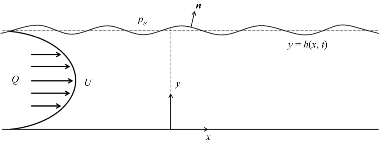
Figure 1. Set-up of the flow in dimensionless variables.
Following earlier studies of the stability of flow past flexible-walled boundaries (e.g. Carpenter & Garrad Reference Carpenter and Garrad1986; Davies & Carpenter Reference Davies and Carpenter1997a; Stewart et al. Reference Stewart, Waters and Jensen2010b) we assume the compliant wall can be modelled as an Euler–Bernoulli beam subject to an external pressure  $p_e$. In particular, we assume the flexible wall has restoring forces due its mass $m_0$, internal viscous damping $d_0$ and longitudinal pre-tension $T_0$.
We introduce dimensionless variables by scaling all lengths on  $a$, velocities on $Q/a$, times on $a^2/Q$ and pressures on $\rho Q^2/a^2$ from which we obtain the dimensionless parameters (each marked with a tilde)
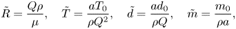 \begin{equation} \tilde R=\frac{Q\rho}{\mu}, \quad \tilde T=\frac{aT_0}{\rho Q^2},\quad\tilde d=\frac{ad_0}{\rho Q},\quad \tilde m=\frac{m_0}{\rho a}, \end{equation}
where  $\tilde R$ is the Reynolds number of the flow, $\tilde T$ is the dimensionless pre-tension of the wall, $\tilde d$ is the dimensionless wall damping and $\tilde m$ is the dimensionless wall mass. All dimensionless variables take the same symbol as their dimensional counterpart and we henceforth drop tildes for convenience.
2.1. Governing equations
The fluid flow is governed by the (two-dimensional) incompressible Navier–Stokes equations, where  ${\boldsymbol u}=(u,v)$ and $p$ denote the dimensionless velocity and pressure of the fluid, respectively, in the form
 \begin{gather} {u}_x+{v}_y=0, \end{gather}
 \begin{gather}{u}_t+u{u}_x+v{u}_y={-}{p}_x+{R}^{{-}1}(u_{xx} + u_{yy}), \end{gather}
 \begin{gather}{v}_t+u{v}_x+v{v}_y={-}{p}_y+{R}^{{-}1}(v_{xx} + v_{yy}). \end{gather}
On the rigid wall we apply boundary conditions of no slip and no penetration in the form
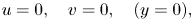 \begin{equation} u=0, \quad v=0, \quad (y=0),\end{equation}
while on the compliant wall we apply kinematic and no-slip conditions in the form
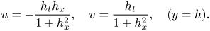 \begin{equation} u={-}\frac{h_t h_x}{1+h_x^2}, \quad v=\frac{h_t}{1+h_x^2}, \quad (y=h).\end{equation}
The shape of the flexible wall is governed by a normal stress balance, in the form
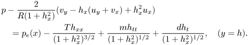 \begin{align} &p-\frac{2}{R(1+h_x^2)}(v_y-h_x(u_y+v_x)+h_x^2u_x) \nonumber\\ &\quad=p_e(x)-\frac{Th_{xx}}{(1+h_x^2)^{{3}/{2}}}+ \frac{mh_{tt}}{({1+h_x^2})^{1/2}}+\frac{dh_t}{({1+h_x^2})^{1/2}}, \quad (y=h). \end{align}
This wall model includes the same features as Benjamin (Reference Benjamin1960, Reference Benjamin1963) and Landahl (Reference Landahl1962). We note that this balance includes the normal viscous stress (terms appearing with coefficient  $R^{-1}$).
2.2. Nonlinear energy equation
To analyse the energy budget of the modes of instability in this collapsible channel system we compute the energy budget by taking the scalar product of the momentum equations (2.2b,c) with the fluid velocity  $\boldsymbol {u}$ in the form
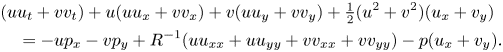 \begin{align} &(u{u}_t+v{v}_t)+u({u}{u}_x+v{v}_x)+v (u{u}_y+{v}{v}_y)+\tfrac{1}{2}(u^2+v^2) (u_x+v_y) \nonumber\\ &\quad ={-}u{p}_x-v{p}_y+R^{{-}1}(uu_{xx} + uu_{yy}+vv_{xx} + vv_{yy} )-p(u_x+v_y). \end{align}
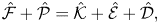
This energy equation can be manipulated into the familiar form
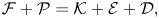 \begin{equation} {\mathcal{F}}+{\mathcal{P}}={\mathcal{K}}+{\mathcal{E}}+{\mathcal{D}},\end{equation}
where
 \begin{gather} {\mathcal{F}}={-}\left(\frac{1}{2}\int_{0}^{h}u (u^2+v^2)\,{\rm d} y\right)_x, \end{gather}
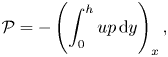 \begin{gather}{\mathcal{P}}={-}\left(\int_{0}^{h} up\,{\rm d} y\right)_x, \end{gather}
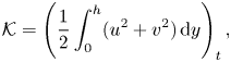 \begin{gather}{\mathcal{K}}=\left(\frac{1}{2}\int_{0}^{h}(u^2+v^2)\,{\rm d} y\right)_t, \end{gather}
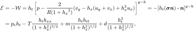 \begin{align} {\mathcal{E}}&={-}{\mathcal{W}}=h_t \left[p-\frac{2}{R(1+{h_x}^2)} (v_y-h_x(u_y+v_x)+{h_x^2} u_x)\right]^{y=h}={-} [h_t({\boldsymbol{\sigma}}{\boldsymbol n})\boldsymbol{\cdot} {\boldsymbol n}]^{y=h} \nonumber\\ &=p_e h_t - T\frac{h_t h_{xx}}{(1+h_x^2)^{{3}/{2}}}+m\frac{h_t h_{tt}}{({1+h_x^2})^{1/2}}+d\frac{h_t^2}{({1 +h_x^2})^{1/2}}, \end{align}
 \begin{equation} {\mathcal{D}}={R}^{{-}1}\left\{\int_0^h(2u_x^2+2v_y^2+(u_y+v_x)^2)\,{\rm d} y-\left(\int_0^h(2uu_x+vv_x+vu_y)\,{\rm d} y\right)_x\right\}, \end{equation}
where  ${\boldsymbol {\sigma }}$ is the Newtonian stress tensor and ${\boldsymbol n}$ is the outward pointing unit normal to the flexible wall (see figure 1). Here, ${\mathcal {F}}$ is the kinetic energy flux extracted from the mean flow, $\mathcal {P}$ is the rate of working of the axial pressure gradient, ${\mathcal {K}}$ is the rate of change of kinetic energy, ${\mathcal {W}}=-{\mathcal {E}}$ is the rate of working of fluid normal stress on the wall and ${\mathcal {D}}$ is the rate of energy loss due to fluid viscosity in the bulk. Note that we re-write ${\mathcal {E}}$ by substituting the normal stress balance (2.2f) and the boundary conditions (2.2e), which then expresses the work done by the fluid on the wall in terms of the wall parameters. Note also that previous studies (e.g. Carpenter & Gajjar Reference Carpenter and Gajjar1990; Huang Reference Huang1998) have considered the work done by fluid pressure on the wall, whereas in this case we consider the work done by the normal stress, including the viscous contributions (see also Lebbal et al. Reference Lebbal, Alizard and Pier2022).
2.3. Linearisation around the uniform basic state
We assume the velocity and pressure of the steady flow when the elastic wall is flat to be of the familiar (fully developed) Poiseuille form
 \begin{equation} (u,v)=(U(y),0)=(6y(1-y),0),\quad p=p_e=P(x)=C-\frac{12}{R}x, \quad h=1, \end{equation}
where  $C$ is a constant, which is a solution to (2.2) for all $C$. We note that the external pressure is not spatially uniform; we are applying an external pressure gradient to maintain a flat base state. Such an assumption was previously applied by Stewart et al. (Reference Stewart, Waters and Jensen2010b) and is consistent with earlier work which ignored the pressure gradient associated with the mean flow in the normal stress balance (e.g. Carpenter & Garrad Reference Carpenter and Garrad1985; Davies & Carpenter Reference Davies and Carpenter1997a).
We add a small perturbation to this steady flow in the form
 \begin{equation} (u,v,p,h)=(U(y),0,P(x),1)+\varepsilon (\hat{\phi}_y,-\hat\phi _x,\hat{p},\hat{\eta})+ \varepsilon^2(\breve\phi _y,-\breve\phi _x,\breve{p},\breve{\eta}) +O(\varepsilon^3),\end{equation}
where  $\varepsilon \ll 1$ is the perturbation amplitude, and $\hat \phi$ and $\breve \phi$ are the perturbation streamfunctions at $O(\varepsilon )$ and $O(\varepsilon ^2)$, respectively. Note that conservation of mass (2.2a) is satisfied automatically at each order.
We substitute the (2.5) into the Navier–Stokes equations (2.2b,c), the boundary conditions (2.2d,e) and the normal stress balance (2.2f) and examine successive orders in the perturbation amplitude  $\varepsilon$.
At  $O(1)$ these equations are satisfied automatically, while at $O(\varepsilon )$ the governing equations of the system become
 \begin{gather} \hat\phi _{yt}+U\hat\phi _{xy}-\hat\phi _{x}U_y+\hat p_x-R^{{-}1}(\hat\phi _{xxy}+\hat\phi _{yyy})=0, \end{gather}
 \begin{gather}\hat\phi _{xt}+U\hat\phi _{xx}-\hat p_y-R^{{-}1}(\hat\phi _{xxx}+\hat\phi _{xyy})=0, \end{gather}
subject to
 \begin{gather} \hat\phi_y=0, \quad \hat\phi_x=0, \quad (y=0), \end{gather}
 \begin{gather}\hat\phi_y+U_y(1)\hat\eta=0,\quad \hat\phi_x + \hat\eta_t=0,\quad (y=1), \end{gather}
while the normal stress balance takes the form
 \begin{equation} \hat p +{2}{R}^{{-}1}(\hat\phi_{y} + U_y(1)\hat\eta)_x + T\hat\eta_{xx}-m\hat\eta_{tt}-d\hat \eta_t =0, \quad (y=1).\end{equation}
Here, we have explicitly included the normal viscous stress contributions in (2.6e), although these cancel identically at this order due to the no-slip boundary condition (2.6d).
Similarly, at  $O(\varepsilon ^2)$, the governing equations of the system become
 \begin{gather} \breve\phi_{yt}+U\breve\phi_{xy}-U_y\breve\phi_x+\breve p_x-R^{{-}1}(\breve\phi_{xxy}+\breve\phi_{yyy}) =\hat\phi_x\hat\phi_{yy}-\hat\phi_y\hat\phi_{xy}, \end{gather}
 \begin{gather}\breve\phi_{xt}+U\breve\phi_{xx}-\breve{p}_y-R^{{-}1} (\breve\phi_{xxx}+\breve\phi_{xyy}) =\hat\phi_x\hat{\phi}_{xy}-\hat\phi_y\hat\phi_{xx}, \end{gather}
subject to boundary conditions
 \begin{gather} \breve\phi_y=0, \quad \breve\phi_x=0, \quad (y=0), \end{gather}
 \begin{gather}\breve\phi_y + U_y(1)\breve\eta ={-}\hat\phi_{yy}\hat\eta - \tfrac{1}{2}U_{yy}(1) {\hat \eta}^2 - \hat\eta_x\hat\eta_t,\quad \breve\phi_x+\breve\eta_t={-}\hat \eta\hat\phi_{xy}, \quad (y=1), \end{gather}
and the normal stress balance
 \begin{align} &\breve p+{2}{R^{{-}1}}(\breve\phi_{xy}+U_y(1)\breve\eta_x) +T\breve\eta_{xx}-m\breve\eta_{tt}-{\rm d} \breve \eta_t \nonumber\\ &\quad ={-}\hat\eta\hat p_y-{2}{R^{{-}1}}(\hat\phi_{xyy}\hat\eta +U_{yy}(1)\hat\eta\hat\eta_x+(\hat\phi_{yy}-\hat\phi_{xx}) \hat\eta_x),\quad (y=1). \end{align}
2.4. The first-order equations
To solve the first-order governing equations, we assume that all hatted variables are wave like in the form
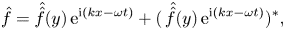 \begin{equation} {\hat f}=\hat{\hat{f}}(y)\, {\rm e}^{{\rm i}(kx-\omega t)}+(\,\hat{\hat{f}}(y)\, {\rm e}^{{\rm i}(kx-\omega t)})^*,\end{equation}
where  $k$ is the wavenumber and $\omega$ is the corresponding frequency of the perturbation, while $^*$ denotes the complex conjugate. We also express our neutral stability curves in terms of the perturbation wavespeed, $c=\omega /k$ for $k$ real (Whitham Reference Whitham1974).
Substituting (2.8) into the first-order governing equations (2.6a)–(2.6e), we have
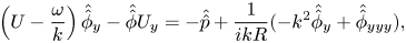 \begin{gather} \left(U-\frac{\omega}{k}\right)\hat{\hat{\phi}}_y- \hat{\hat{\phi}}U_y={-}\hat{\hat{p}}+\frac{1}{ikR} ({-}k^2\hat{\hat{\phi}}_y+\hat{\hat{\phi}}_{yyy}), \end{gather}
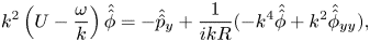 \begin{gather}k^2\left(U-\frac{\omega}{k}\right)\hat{\hat{\phi}} ={-}\hat{\hat{p}}_y+\frac{1}{ikR}({-}k^4\hat{\hat{\phi}} +k^2\hat{\hat{\phi}}_{yy}), \end{gather}
subject to boundary conditions
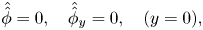 \begin{gather} \hat{\hat{\phi}}=0, \quad \hat{\hat{\phi}}_y=0,\quad (y=0), \end{gather}
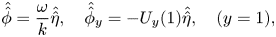 \begin{gather}\hat{\hat{\phi}}=\frac{\omega}{k}\hat{\hat{\eta}}, \quad \hat{\hat{\phi}}_y={-}U_y(1)\hat{\hat{\eta}},\quad (y=1), \end{gather}
and the normal stress balance
 \begin{equation} \hat{\hat{p}}=\frac{1}{ikR}({-}k^2\hat{\hat{\phi}}_y+ \hat{\hat{\phi}}_{yyy})=(Tk^2-m\omega^2-id\omega) \hat{\hat{\eta}}, \quad (y=1).\end{equation}
Combining (2.9a) and (2.9b) by eliminating  $\hat {\hat {p}}$, we obtain the classical Orr–Sommerfeld equation (see below, Drazin & Reid Reference Drazin and Reid1981; Schmid & Henningson Reference Schmid and Henningson2001).
We adopt two complementary approaches to solve this linear system. First, we use the no-slip boundary condition (2.9d) to eliminate the wall amplitude  $\hat {\hat {\eta }}$ to derive a (closed) fourth-order homogeneous system for ${\hat {\hat \phi }}(y)$ in the form
 \begin{equation} \left(U-\frac{\omega}{k}\right) (\hat{\hat{\phi}}_{yy}-k^2\hat{\hat{\phi}})- U_{yy}\hat{\hat{\phi}}-\frac{1}{ikR} (\hat{\hat{\phi}}_{yyyy}-2k^2\hat{\hat{\phi}}_{yy} +k^4\hat{\hat{\phi}})=0, \end{equation}
subject to four boundary conditions
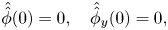 \begin{gather} \hat{\hat{\phi}}(0)=0, \quad \hat{\hat{\phi}}_y(0)=0, \end{gather}
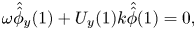 \begin{gather}\omega\hat{\hat{\phi}}_y(1) + U_y(1)k \hat{\hat{\phi}}(1)=0, \end{gather}
 \begin{gather}\frac{1}{i k R}U_y(1)({-}k^2\hat{\hat{\phi}}_y(1)+\hat{\hat{\phi}}_{yyy}(1) ) + (Tk^2 - m\omega^2-id\omega)\hat{\hat{\phi}}_y(1)=0. \end{gather}
For fixed Reynolds number,  $R$, and wavenumber, $k$, we solve the eigenvalue problem numerically by discretising (2.10) using a Chebyshev spectral method similar to that used by Stewart et al. (Reference Stewart, Waters and Jensen2010b) modified to include the wall mass. For a given value of the wavenumber and the other model parameters ( $R$,
$R$,  $T$,
$T$,  $m$ and $d$), for $N$ Chebyshev modes the numerical method isolates eigenvalues $\omega _i$ and corresponding eigenfunctions ${\hat {\hat \phi }}_i(y;k,\omega )$ for
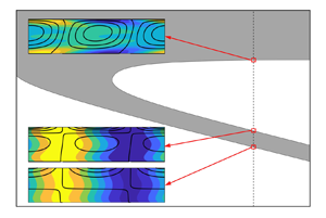
  $i=1,2,\ldots,N$. Typical eigenvalue spectra are shown in figure 6(c,d), where the eigenvalues can be divided into the familiar A, P and S branches (Mack Reference Mack1976; Drazin & Reid Reference Drazin and Reid1981; Schmid & Henningson Reference Schmid and Henningson2001). As the number of Chebyshev modes increases the additional eigenvalues appear with increasingly large and negative imaginary part (along the S branch) and the portion of the spectrum close to neutral stability becomes well resolved. See Wang (Reference Wang2019) for further details. Knowledge of the entire eigenvalue spectrum (as opposed to just neutrally stable modes) serves to elucidate the mode interactions discussed in later sections. For the plots in this paper we normalise the eigenfunction so that $\hat {\hat {\phi }}_y(1)=-U_y(1)=6$, consistent with the inhomogeneous formulation (2.11). We focus particular attention on neutrally stable solutions, where ${\rm Im} (\omega )=0$, which we isolate using a bisection method and trace various slices through the parameter space. In particular, we compute the neutrally stable wavenumber, denoted $k_n$, corresponding (real) neutrally stable frequency, denoted $\omega _n$ and corresponding (real) wavespeed, denoted $c_n=\omega _n/k_n$, as a function of the model parameters in figures 2–10.
To make analytical progress we also adopt an alternative approach which separates computation of the eigenfunction from the stability calculation. In this case we first normalise the eigenfunction based on the amplitude of the wall profile, scaling the perturbation streamfunction according to  $\hat {\hat {\phi }} = \hat {\hat {\eta }}{\tilde {\hat \phi }}$ and express (2.9) as a closed inhomogeneous system for ${\tilde {\hat \phi }}(y)$ alone in the form
 \begin{equation} \left(U-\frac{\omega}{k}\right)(\tilde{\hat{\phi}}_{yy} -k^2\tilde{\hat{\phi}})-U_{yy}\tilde{\hat{\phi}}- \frac{1}{ikR}(\tilde{\hat{\phi}}_{yyyy}-2k^2 \tilde{\hat{\phi}}_{yy}+k^4\tilde{\hat{\phi}})=0, \end{equation}
subject to
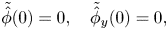 \begin{gather} \tilde{\hat{\phi}}(0)=0, \quad \tilde{\hat{\phi}}_y(0)=0, \end{gather}
 \begin{gather}\tilde{\hat{\phi}}(1)=\frac{\omega}{k}, \quad \tilde{\hat{\phi}}_y(1)={-}U_y(1). \end{gather}
In this way, the streamfunction  ${\tilde {\hat \phi }}(y)$ can be computed for any $k$ and $\omega$, independent of the stability criteria. Landahl (Reference Landahl1962) achieved an analogous separation in his (more approximate) approach by expressing the problem in terms of the wall admittance, which facilitated calculation of the activation energy. Given a solution of (2.11), following Cairns (Reference Cairns1979), the normal stress balance on the flexible wall can be expressed as a dispersion relation of the system in the form
 \begin{equation} D(\omega,k)\equiv\frac{1}{ikR}(\tilde{\hat{\phi}}_{yyy}(1)- k^2\tilde{\hat{\phi}}_y(1))-(Tk^2-m\omega^2-id\omega),\end{equation}
which is zero for normal modes. Crucially, this approach formulates the dispersion relation as a scalar-valued function involving the frequency  $\omega$ and the wavenumber $k$ (in this case in terms of the normal stress balance on the wall), rather than as a inhomogeneous eigenvalue problem which must be solved numerically (e.g. Davies & Carpenter Reference Davies and Carpenter1997a; Stewart et al. Reference Stewart, Waters and Jensen2010b); this scalar dispersion relation has two components: the first group of terms arises due to the viscous normal stress on the wall, while the second group of terms arises from the contributions to the Euler–Bernoulli beam. The inviscid dispersion relation (see Appendix A) does not have the viscous terms but contains an extra term due to inertial contribution to the pressure, which cancels identically here due to the no-slip condition on the flexible wall. We use this dispersion relation to compute the activation energy of the neutrally stable surface-based modes following Landahl (Reference Landahl1962) and Cairns (Reference Cairns1979).
Note that our choice of normalisation for the numerical solutions of the homogeneous system (2.10) means that at neutral stability the two streamfunction profiles are identical ( $\hat {\hat {\phi }}(y;\omega _n,k_n)=\tilde {\hat {\phi }}(y;\omega _n,k_n)$). For notational simplicity, we henceforth denote $\tilde {\hat {\phi }}(y)=\phi (y)$.
2.5. The second-order equations
At second order we express the variables in the form
 \begin{equation} \breve g(x,y,t)=\breve{\breve{g}}(y)\, {\rm e}^{2{\rm i}(kx-\omega t)}+\bar{{\breve{g}}}(y)+(\breve{\breve{g}}(y)\, {\rm e}^{2{\rm i}(kx-\omega t)})^*. \end{equation}
Substituting (2.12) into the second-order equations (2.7), we consider steady streaming terms which are independent of both  $x$ and $t$ (denoted with an additional overline) to obtain a system which depends only on $y$, in the form
 \begin{equation} {-\bar{\breve p}_x +} \frac{1}{R}\bar{\breve{\phi}}_{yyy} = \overline{\hat{\phi}_y \hat{\phi}_{xy}} {- \overline{\hat{\phi}_x \hat{\phi}_{yy}}}, \quad \bar{{\breve p}}_y=0, \quad (0\le y \le 1),\end{equation}
subject to
 \begin{equation} \bar{\breve{\phi}}_{y}(0)=0, \quad \bar{\breve{\phi}}_{y}(1)={-} U_{y}(1)\bar{{\breve \eta}} - \tfrac{1}{2}U_{yy}(1)\overline{{\hat \eta}^2} - \overline{{\hat \phi}_{yy}(1) {\hat \eta}} - \overline{{\hat \eta}_t {\hat \eta}_x},\end{equation}
noting that  $x$ and $t$ independent terms occur at this order from products of the first-order eigenfunctions. Note also that the term $\bar {\breve p}_x$ is independent of $x$, representing the steady modification to the pressure gradient along the channel. The corresponding kinematic boundary condition is identically zero. Steady streaming can either result in a modification to the steady pressure gradient ( $\bar {\breve p}_x$), a modification to the steady flux along the channel ( $\bar {\breve q}=\bar {\breve \phi }(1)-\bar {\breve \phi }(0)$) or the mean wall position ( ${\bar {\breve \eta }}$), only one of which can be fixed by solving the equations. In this case we are assuming a fixed baseline flow rate which imposes $\bar {\breve q}=0$ and ${\bar {\breve \eta }}=0$ to ensure the total mass of fluid in the channel remains fixed. By integrating (2.13a) and applying boundary conditions (2.13b) we obtain a prediction of the streamfunction profile $\bar {\breve {\phi }}_{y}$ and pressure gradient $\overline {\breve {p}}_x$ in terms the numerically computed eigenfunctions from the first-order problem (see Wang (Reference Wang2019), for details). This profile is used to calculate the full expression for the work done on the wall by the fluid in the time- and space-averaged energy budget (see § 2.6).
2.6. The Reynolds–Orr energy equation
We obtain the linearised energy equation by substituting the expansion (2.5) into the energy equation (2.3). The first non-trivial balance emerges at second order in perturbation amplitude, where we have
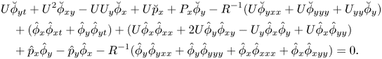 \begin{align} &U\breve\phi_{yt}+U^2\breve\phi_{xy}-UU_y\breve{\phi}_x +U\breve{p}_x+P_x\breve{\phi}_y-{R}^{{-}1}(U\breve{\phi}_{yxx} +U\breve{\phi}_{yyy}+U_{yy}\breve{\phi}_y)\nonumber\\ &\quad+(\hat{\phi}_x\hat\phi_{xt}+\hat{\phi}_y\hat\phi_{yt}) + (U\hat{\phi}_x\hat\phi_{xx}+2U\hat{\phi}_y\hat\phi_{xy}-U_y \hat{\phi}_x\hat{\phi}_y+U\hat{\phi}_x\hat\phi_{yy}) \nonumber\\ &\quad+\hat{p}_x\hat{\phi}_y-\hat{p}_y\hat{\phi}_x-{R}^{{-}1} (\hat{\phi}_y\hat{\phi}_{yxx}+\hat\phi_y\hat\phi_{yyy}+ \hat\phi_x\hat\phi_{xxx}+\hat\phi_x\hat{\phi}_{xyy})=0. \end{align}
Domaradzki & Metcalfe (Reference Domaradzki and Metcalfe1987) (see also Stewart et al. Reference Stewart, Waters and Jensen2010b; Lebbal et al. Reference Lebbal, Alizard and Pier2022) demonstrated that the terms involving breved variables can be eliminated in favour of terms involving the first-order variables alone (using the  $O(\epsilon ^2)$ governing equations), analogous to the derivation of the classical Reynolds–Orr equation (see details in Schmid & Henningson Reference Schmid and Henningson2001). The corresponding energy budget is obtained by integrating across the static channel $(0\le y\le 1)$ to obtain the work done by nonlinear Reynolds stresses, which was termed ${\hat {\mathcal {S}}}$ by Stewart et al. (Reference Stewart, Waters and Jensen2010b). However, in this approach, it is not then possible to explicitly construct the full expression for the work done by the fluid on the wall as some contributions are embedded within ${\hat {\mathcal {S}}}$. In this study, we adopt an alternative approach where we retain the full expressions for the terms in the energy equation (2.14) involving both hatted and breved variables. In this case the energy budget at $O(\varepsilon ^2)$ can be expressed as
 \begin{equation} {\hat{\mathcal{F}}} + {\hat{\mathcal{P}}} ={\hat{\mathcal{K}}} + {\hat{\mathcal{E}}} + {\hat{\mathcal{D}}}, \end{equation}
where
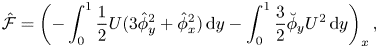 \begin{gather} {\hat{\mathcal{F}}}=\left( -\int_{0}^{1}\frac{1}{2}U(3{\hat\phi_y}^2+{\hat\phi_x}^2)\,{\rm d} y-\int_0^1\frac{3}{2}\breve\phi_yU^2\,{\rm d} y\right)_x, \end{gather}
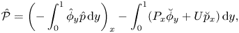 \begin{gather}{\hat{\mathcal{P}}}= \left(-\int_0^1\hat\phi_y\hat p\,{\rm d} y\right)_x- \int_0^1(P_x\breve\phi_y+{U{\breve p}_x})\,{\rm d} y, \end{gather}
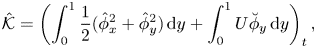 \begin{gather}{\hat{\mathcal{K}}}= \left(\int_{0}^{1}\frac{1}{2} ({\hat\phi_x}^2+{\hat\phi_y}^2)\,{\rm d} y + \int_0^1 U\breve\phi_y\,{\rm d} y\right)_t, \end{gather}
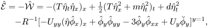 \begin{align} {\hat{\mathcal{E}}}&={-}{\hat{\mathcal{W}}}={-}(T\hat\eta_t\hat\eta_x)_x+\tfrac{1}{2} (T\hat\eta_x^2+m\hat\eta_t^2)_t+d\hat\eta_t^2\nonumber\\ &\quad {-}{R}^{{-}1}[-{U_{yy}}(\hat\eta\hat\phi_x)_x + \hat\phi_y\hat\phi_{yy}-3\hat\phi_y\hat\phi_{xx} + U_y\breve\phi_y]^{y=1}, \end{align}
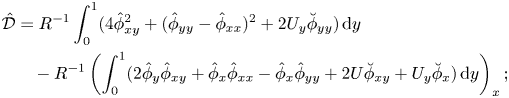 \begin{align} {\hat{\mathcal{D}}}&={R}^{{-}1}\int_0^1(4\hat\phi_{xy}^2+ (\hat\phi_{yy}-\hat\phi_{xx})^2+2U_y\breve\phi_{yy})\,{\rm d} y \nonumber\\ &\quad -{R}^{{-}1}\left(\int_0^1(2\hat\phi_y\hat\phi_{xy}+ \hat\phi_x\hat\phi_{xx}-\hat\phi_x\hat\phi_{yy} + 2U\breve\phi_{xy}+U_y\breve\phi_x)\,{\rm d} y\right)_x; \end{align}
where  ${\hat {\mathcal {F}}}$ represents the net energy extracted from the mean flow across the channel, ${\hat {\mathcal {P}}}$ represents the work done by axial pressure forces over a wavelength, ${\hat {\mathcal {W}}}=-{\hat {\mathcal {E}}}$ represents the total work done by the fluid normal stress on the wall (note the wall elasticity parameters appear as the normal stress condition (2.6e) has been used to eliminate the fluid pressure on the wall) and ${\hat {\mathcal {D}}}$ represents the total viscous dissipation across the bulk of the channel.
Following Landahl (Reference Landahl1962), we average (2.15) over a wavelength of perturbation where it reduces to
 \begin{align} &\left(\int_{0}^{1}\frac{1}{2}({\hat\phi_x}^2+{\hat\phi_y}^2) \,{\rm d} y + \frac{1}{2}(T\hat\eta_x^2+m\hat\eta_t^2)\right)_t ={-}d(\hat\eta_t)^2 \nonumber\\ &\quad -{R}^{{-}1}\int_0^1(4\hat\phi_{xy}^2+ (\hat\phi_{yy}-\hat\phi_{xx})^2+2U_y\breve\phi_{yy}) \,{\rm d} y \nonumber\\ &\quad -{R}^{{-}1}[\hat\phi_y\hat\phi_{yy}-3\hat\phi_y\hat\phi_{xx} + U_y\breve\phi_y]^{y=1} ; \end{align}
the term on the left-hand side is the rate of change of the activation energy of the system (sum of kinetic and elastic energies for the fluid and the wall), while the terms on the right-hand side represent (non-conservative) energy losses due to the wall damping, fluid viscosity across the bulk and viscous stresses exerted on the flexible wall, respectively. In a conservative system (with no wall damping or viscous dissipation) the activation energy is constant and must always be positive definite in this case. This suggests that undamped modes must always be class B (according to Benjamin's framework) in the limit of large Reynolds number. However, in the fully inviscid limit (Appendix A) the activation energy can be negative due to the extra (inertial) contribution to the fluid pressure on the wall which cancels in the viscous problem due to the no-slip condition. However, this approach cannot be used as a measure of activation energy for neutrally stable modes in a viscous system, since this formulation neglects the contribution of viscosity in establishing the neutrally stable mode. We propose an alternative method to construct the sign of the activation energy of neutrally stable viscous modes in the following subsection.
Instead, taking the average of (2.15) over both a period and wavelength (again denoted with an overbar), the averaged energy budget (2.15) reduces to
 \begin{equation} \bar{\hat{\mathcal{P}}} =\bar{\hat{\mathcal{E}}} + \bar{\hat{\mathcal{D}}}, \end{equation}
where
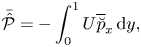 \begin{gather} {\bar{\hat{\mathcal{P}}}}={-}\int_0^1 U \overline{\breve{p}}_x\,\text{d}y, \end{gather}
 \begin{gather}{\bar{\hat{\mathcal{E}}}}={-}{\bar{\hat{\mathcal{W}}}} ={\rm d}\overline{{\hat\eta}_t^2} -{R}^{{-}1} [\overline{\hat\phi_y\hat\phi_{yy}} -3\overline{\hat\phi_{y}\hat\phi_{xx}}+U_y \bar{{\breve \phi}}_y]^{y=1}, \end{gather}
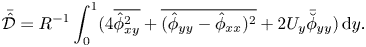 \begin{gather}{\bar{\hat{\mathcal{D}}}}={R}^{{-}1}\int_0^1 (4\overline{{\hat\phi}_{xy}^2}+ \overline{({\hat\phi}_{yy}-{\hat\phi}_{xx})^2}+2U_y \bar{{\breve\phi}}_{yy})\,{\rm d} y. \end{gather}
We particularly consider the averaged work done by the fluid on the wall over a period and wavelength,  ${\bar {\hat {\mathcal {W}}}}=-{\bar {\hat {\mathcal {E}}}}$, which we compute below. This time-averaged energy budget (2.17) also serves as a useful check of our neutrally stable solutions and we confirm that the total error is $O(10^{-5})$ for all cases tested (Wang Reference Wang2019). Note also that this energy budget explicitly separates the work done by the fluid on the wall and the work done by the axial pressure gradient, whereas in Stewart et al. (Reference Stewart, Waters and Jensen2010b) these contributions were lumped into other terms.
2.7. Activation energy
As shown previously, the Reynolds–Orr energy budget calculation does not lead to a self-consistent prediction of the activation energy for a viscous perturbation mode. Instead, we follow the formulation of Landahl (Reference Landahl1962), who computed the activation energy of a neutrally stable mode as proportional to the difference in mechanical impedance arising from a small perturbation from the neutral point. As noted by Landahl (Reference Landahl1962), this approach does not necessarily hold for a viscous flow as it neglects some terms, but, as in that study, we assume that the sign of the activation energy is predicted correctly for a viscous flow. Indeed, we show below that the sign of the activation energy for the FISI is consistent with the classification framework of Benjamin (Reference Benjamin1960) based on the response to wall damping. Similarly, Cairns (Reference Cairns1979) defined activation energy for a neutral inviscid wave (using piecewise-constant velocity profiles with no shear or critical layers), arguing that since both boundary layer flow and plane Poiseuille flow have nearly neutral inviscid normal modes in the long-wave limit, their activation energy can be approximated using the inviscid equations (provided a small indentation is taken in the complex plane to pass around the critical point) and the sign of their activation energy predicts the destabilising effects of viscosity in the Orr–Sommerfeld equation. We follow the notation of Cairns (Reference Cairns1979) and express the activation energy in terms of the fluid pressure on the wall through the dispersion relation  $D(\omega,k)$ (cf. (2.11d)); since ${D}=0$ for normal modes, it emerges that this difference in normal stress (impedance) must be Taylor expanded about the neutral stability point to obtain an expression for the activation energy in the form (Landahl Reference Landahl1962; Cairns Reference Cairns1979)
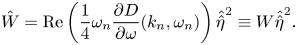 \begin{equation} {\hat W} = {{\rm Re} }\left(\frac{1}{4}\omega_n \frac{\partial {{D}}}{\partial \omega}(k_n,\omega_n)\right) {\hat{\hat \eta}}^2 \equiv W {\hat{\hat \eta}}^2. \end{equation}
Based on the dispersion relation (2.11d), this formula suggests there are two contributions to the activation energy for a viscous mode at neutral stability, one arising due to viscous effects and the other due to wall elasticity (wall mass and pre-tension). However, we note that if  ${{\phi }}$ is purely real then the viscous contribution to ${D}$ is purely complex, and so does not contribute to the activation energy. For an inviscid fluid (see Appendix A) there is another contribution which cancels here due to the no-slip boundary conditions. We use (2.18) below to compute the activation energy of neutrally stable FISI using a combination of numerical and asymptotic analysis. In particular, we apply (2.18) to compute explicit expressions for the activation energy in the limit of large wall mass (§ 3) and large wall damping (§ 4). Furthermore, to numerically compute the activation energy of a neutrally stable normal mode, we perturb the neutrally stable frequency by a real (small) amount $\pm {\rm \Delta} \omega$, and use a second-order centred finite difference stencil to approximate the derivative in (2.18) with error $O({\rm \Delta} \omega ^2)$, in the form
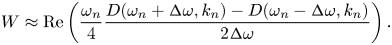 \begin{equation} {W} \approx {\rm Re} \left(\frac{\omega_n}{4} \frac{{D}(\omega_n+{\rm \Delta} \omega,k_n) - {D}(\omega_n-{\rm \Delta} \omega,k_n)}{2 {\rm \Delta} \omega} \right). \end{equation}
This numerical interpretation is equivalent to computing the difference in mechanical impedance arising from a small perturbation from the neutral stability point, consistent with Landahl (Reference Landahl1962). Note this approach to construct the activation energy only works for normal modes which are surface based (flutter, divergence, TWF, SD) and does not work for the hydrodynamic modes (TS).
3. Stability of Poiseuille flow in the absence of wall damping
We consider the stability of Poiseuille flow through an asymmetric compliant channel with a flexible wall with mass and pre-tension, using the numerical method described in § 2.4 to analyse the neutrally stable solutions of the system in the absence of wall damping (§ 3.1), examining the mode interaction between TWF and TS (§ 3.2), before exploring the asymptotic structure of the neutrally stable TWF modes in the limit of large wall mass (§ 3.3).
3.1. Numerical results
To assess the stability of viscous system in the absence of wall damping, in figure 2 we trace neutral stability curves as a function Reynolds number in terms of the critical wavenumber (figure 2a) and the corresponding wavespeed (figure 2b) for selected values of the wall mass. As expected, the system is unstable to class A TS modes within a tongue-shaped region for sufficiently large Reynolds numbers, analogous to those found in a rigid-walled channel (Drazin & Reid Reference Drazin and Reid1981). For small and large values of the wall mass the corresponding TS neutral stability curve is only modified very slightly from the case with zero wall mass (figure 2a). For example, the corresponding critical Reynolds number for instability is modified from  $R_c\approx 7743$ for $m=0$ to $R_c \approx 7693$ for $m=1000$. However, we note that for a range of intermediate values of the wall mass the behaviour of the TS mode is more complicated, exhibiting a mode interaction with TWF which is explored in more detail in § 3.2.
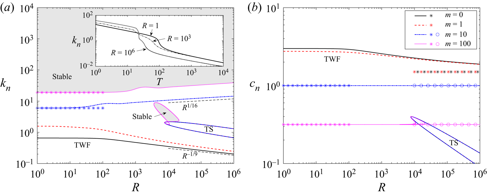
Figure 2. Neutral stability curves for Poiseuille flow as a function of the Reynolds number for selected values of the wall mass with fixed wall tension ( $T=10$) and zero wall damping ( $d=0$), illustrating: (a) critical wavenumber $k_n$; (b) critical wavespeed $c_n$. In each panel we consider $m=0$ (black), $m=1$ (red), $m=10$ (blue) and $m=100$ (magenta). The asterisks correspond to the leading-order prediction for neutrally stable TWF in the limit of large wall mass and low Reynolds number (3.2) while the open circles in (b) correspond to the leading-order wavespeed for large mass and large Reynolds number. The shaded regions in (a) indicate where the base state is asymptotically stable for $m=100$. The inset to (a) shows the neutrally stable wavenumber as a function of wall tension $T$ for three values of the Reynolds number ( $R=1$, $R=10^3$ and $R=10^6$).
The base flow is also unstable to a single surface-based normal mode, which takes the form of class B TWF at neutral stability. The corresponding neutral stability curves each enclose a region for small wavenumbers and each exhibit two regimes (figure 2a,b). For small Reynolds numbers these neutral stability curves are independent of  $R$, where the critical wavespeed reduces from twice the maximal flow speed ( $c=3$ for $R=0$, where the system is notably still unstable to TWF) towards zero as the wall mass increases. Note that for our choice of non-dimensionalisation the limit $R\to 0$ corresponds to increasing fluid viscosity rather than vanishing flow velocity. Indeed, in a different approach where the wall parameters are scaled consistent with Squire's theorem (Rotenberry & Saffman Reference Rotenberry and Saffman1990), the TWF neutral stability curves no longer persist all the way to $R=0$ (Lucey & Carpenter Reference Lucey and Carpenter1995; Davies & Carpenter Reference Davies and Carpenter1997a).
For large Reynolds numbers and low wall mass, the neutrally stable TWF modes are long wavelength but the corresponding limiting wavespeed becomes less than the maximal flow speed ( $c<3/2$) as the wall mass increases and the weak critical layer structure of Stewart et al. (Reference Stewart, Waters and Jensen2010b) is replaced by conventional critical layers (discussed in § 3.3). Conversely, for large values of the wall mass the critical wavenumber increases for large Reynolds numbers, encompassing modes of shorter wavelength (this short-wavelength mode is explored in detail in § 3.3). The transition between the long- and short-wavelength scalings occurs when $m\approx T$, reminiscent of the change in stability observed in potential flow with zero wall damping (Appendix A). However, in the viscous case the instability is class B and occurs as a result of a single normal mode becoming unstable rather than as a result of mode coalescence. Conversely, for $T>m$ the viscous system is long wavelength unstable while the potential flow system is stable. Hence, despite some qualitative similarity of the neutral stability curves, the flutter and TWF instabilities are distinct.
To further explore the behaviour of neutrally stable TWF as the wall becomes heavier, in figure 3 we trace the corresponding neutral stability curves as a function of wall mass for various Reynolds numbers, plotting the critical wavenumber (figure 3a) and the critical wavespeed (figure 3b) in the absence of wall damping. For low values of the wall mass the system is long wavelength unstable to TWF, where the neutral stability curves are independent of mass for small  $m$ (figure 3a,b). Conversely, for large wall mass the critical wavenumber (figure 3a) and frequency (figure 3b) both increase with $m^{1/2}$ and the neutral stability curves become independent of Reynolds number; we exploit this asymptotic scaling in § 3.3. For the neutrally stable TWF mode the total work done by the fluid on the wall over a period is non-zero (figure 3c), in agreement with the mechanism of TWF described by Huang (Reference Huang1998). However, we note that this quantity changes sign when $m\approx T$, suggesting a change in mechanism (figure 3(c) inset). In particular, the total work done by the fluid normal stress on the wall is positive ( ${\bar {\hat {\mathcal {W}}}}=-{\bar {\hat {\mathcal {E}}}}$) for large Reynolds numbers and low wall mass. On the other hand, the activation energy of TWF is always positive for all values of wall mass, consistent with its classification as a class B instability (figure 3d). In summary, this figure shows that in the absence of wall damping the viscous system is unstable to class B TWF which always has positive activation energy but where the work done by the fluid on the wall can change sign as a function of wall mass.
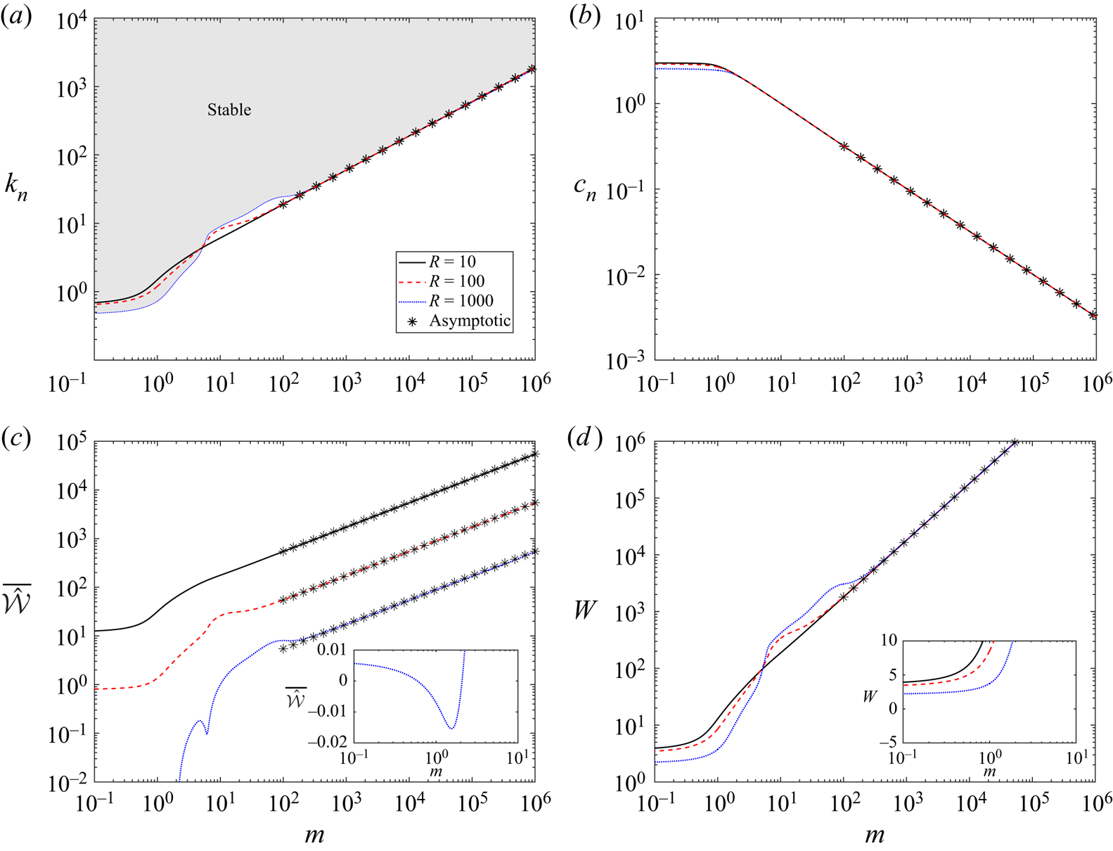
Figure 3. Neutral stability curves of TWF as a function of wall mass for various values of the Reynolds number with fixed pre-tension ( $T=10$) and no wall damping ( $d=0$): (a) critical wavenumber $k_n$; (b) critical wavespeed $c_n$; (c) the negative of the work done by the fluid stress on the wall $\bar {\hat {\mathcal {E}}}=-\bar {\hat {\mathcal {W}}}$; (d) the activation energy $W$. In each panel we consider $R=10$ (solid), $R=100$ (dashed) and $R=1000$ (dotted). The asterisks in (a,b,d) correspond to the leading-order prediction for neutrally stable TWF in the limit of large wall mass (3.2). The shaded region in (a) indicates where the base state is asymptotically stable for $R=1000$. The insets to (c) and (d) show the work done by the fluid on the wall and the activation energy on a linear scale for small values.
3.2. Mode interaction between TS and TWF
In § 3.1 we noted that as the wall mass increases the critical wavespeed of TWF reduces below the maximal flow speed and becomes independent of Reynolds number (figure 2). It emerges that for some parameter values the TWF mode and the TS mode interact (evident from the modification to the TS neutral stability curve in figure 2 for  $m=100$). Such a mode interaction between class A and class B modes is energetically favourable.
To elucidate this mode interaction in more detail, figure 4 explores the neutral stability curves of TWF and TS modes in terms of the critical wavenumber (figure 4a) and wavespeed (figure 4b) as a function of the wall mass for fixed pre-tension and Reynolds number. Across most of the parameter space these neutral stability curves are distinct, but we note that for  $50 \lesssim m \lesssim 120$ the neutral stability curve for TS is no longer independent of wall mass (this range is within the unstable zone of the primary TWF mode). Across this range the frequency of the TS and TWF modes become comparable (for a given wavenumber) and the resulting mode interaction breaks the TS neutral curve into two pieces. These two segments connect to the unstable zones for TS at large and small mass, respectively, but also exhibit a distinct loop at each end within which the base flow is asymptotically stable (shaded regions in figure 4). To examine these islands of stability, we plot the growth rate of the two most unstable normal modes ( ${\rm Im} (\omega )$) as a function of wavenumber for various values of the wall mass (figure 4c–e). For low mass (figure 4c) the TWF and TS modes remain distinct, and both are unstable across a narrow range of wavenumbers. The mode interaction is evident for $m=65$ (figure 4d), where the traces of the two modes deviate and almost touch one another, resulting in a narrow range of $k$ where both modes are stable within the larger TWF unstable zone, but also a substantial increase in the growth rate for larger wavenumbers. The mode interaction is similarly evident for $m=100$ (figure 4e), where the stable island is now relatively large compared with the outer TWF neutral curve (figure 4a). In summary, this figure demonstrates that TS and TWF modes can interact resulting in large stable islands within previously unstable regions.
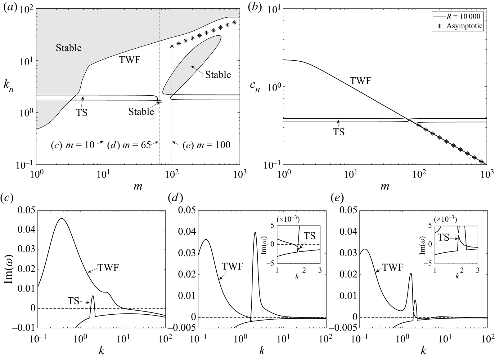
Figure 4. Mode interaction between TS and TWF, plotting the neutral stability curves for Poiseuille as a function of wall mass for fixed pre-tension ( $T=10$) and Reynolds number ( $R=10^6$) with no wall damping ( $d=0$), illustrating: (a) the critical wavenumber $k_n$; (b) the critical wavespeed $c$. The shaded regions in (a) indicate where the base state is asymptotically stable. The asterisks in (a), (b) correspond to the leading-order prediction for neutrally stable TWF in the limit of large wall mass (3.2). To illustrate the mode interaction we plot traces of the perturbation growth rate ${\rm Im} (\omega )$ as a function of wavenumber for the two most unstable normal modes of the system for: (c) $m=10$; (d) $m=65$ and (e) $m=100$. The insets in (d) and (e) show a close-up of the mode interaction.
3.3. The limit of large wall mass
The viscous system with no wall damping exhibits an asymptotic scaling in the limit of large mass ( $m\gg 1$) for fixed wall tension (figure 4), which we exploit by adopting the short-wavelength rescaling
 \begin{equation} k = m^{1/2} k_0, \quad \omega =\omega_0+ m^{{-}1/2}\omega_1 + O(m^{{-}1}), \end{equation}
where  $k_0$ and $\omega _0$ are to be determined at neutral stability. In this limit it emerges that the perturbation eigenfunction is zero across the interior of the channel and close to the lower rigid wall and exhibits a rapidly varying (viscous) solution over a narrow boundary layer adjacent to the compliant wall; a typical eigenfunction profile in this regime is shown in figure 5(a). Across this wall layer we expand the variables according to
 \begin{equation} y =1- m^{{-}1/2} Y, \quad \phi(y) ={-} m^{{-}1/2} \varPhi_{0}(Y) + O(m^{{-}1}), \quad D=m D_0 + m^{1/2} D_1 + O(1). \end{equation}
In this limit, the inhomogeneous Orr–Sommerfeld system (2.11) takes the leading-order form
 \begin{equation} \varPhi_{0,YYYY}-2k_0^2\varPhi_{0,YY}+k_0^4\varPhi_{0}=0, \quad (Y\ge 0), \end{equation}
subject to boundary conditions
 \begin{equation} \varPhi_{0,Y}(0)={-}U_y(1)=6,\quad \varPhi_{0}(0)={-}\frac{\omega_0}{k_0}, \quad \varPhi_{0} \rightarrow 0 \ \text{as} \ Y\rightarrow \infty. \end{equation}
These equations can be solved explicitly in the form
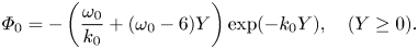 \begin{equation} \varPhi_{0}={-}\left(\frac{\omega_0}{k_0}+ (\omega_0-6)Y\right)\exp({-}k_0Y), \quad (Y\ge 0). \end{equation}
For  $k_0$ and $\omega _0$ as calculated below, this profile shows excellent agreement with the numerically computed perturbation streamfunction for large wall mass (figure 5a). As in the full system, the leading-order normal stress balance on the wall (2.11d) can be expressed as a dispersion relation
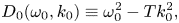 \begin{equation} D_0(\omega_0,k_0) \equiv \omega_0^2 - T k_0^2, \end{equation}
implying that  $\omega _0=\sqrt {T} k_0$ for normal modes, and so the leading-order system is always neutrally stable. This is consistent with the potential flow formulation in Appendix A, where the inviscid class B mode is neutrally stable.
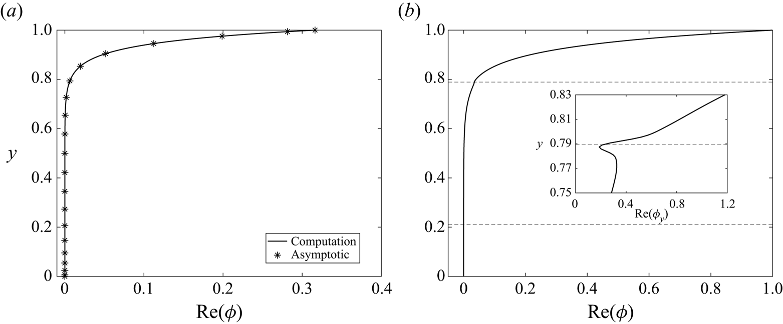
Figure 5. Neutrally stable eigenfunctions for TWF for pre-tension  $T=10$ and no wall damping, illustrating: (a) numerically computed eigenfunction profile ${\rm Re} (\phi (y))$ for $m=100$ and $R=10$ compared with the large $m$ approximation to the eigenfunction (3.1e) for the same wall mass; (b) numerically computed eigenfunction profile ${\rm Re} (\phi (y))$ for $m=10$, $R=10^6$. The dashed lines in (b) indicate the positions of the two critical layers. The inset to (b) shows the streamwise velocity profile ${\rm Re} (\phi _y(y))$ in the neighbourhood of the critical layer.
Expanding the normal stress balance (2.11d) to the following order ( $O(m^{1/2})$), we obtain the next-order correction to the dispersion relation (which includes viscous effects) in the form
 \begin{equation} D_1(\omega_0,\omega_1,k_0) \equiv \frac{1}{i k_0 R} (\varPhi_{0,YYY}(0)-k_0^2\varPhi_{0,Y}(0)) + 2 \omega_0\omega_1. \end{equation}
Normal modes require  $D_1=0$, so that
 \begin{equation} \omega_1 ={-}\frac{i k_0}{R}\frac{(\omega_0-6)}{\omega_0}, \end{equation}
independent of both the wall tension and the wall mass (in contrast to the inviscid flutter modes of Appendix A). Hence, neutrally stable TWF (with  ${\rm Im} (\omega _1)=0$) requires $\omega _{0n}=6$ and $k_{0n}=6/\sqrt {T}$ in the limit of large wall mass, independent of the Reynolds number. We note particularly that the TWF can be shown to be unstable even for $R=0$ (unlike the TWF modes reported by Stewart et al. Reference Stewart, Waters and Jensen2010b) since the leading-order balance is between the tension and mass components of the flexible wall.
Expressing in terms of the original model parameters, we obtain the criticality conditions
 \begin{equation} k_n = 6\left(\frac{m}{T}\right)^{1/2}, \quad \omega_n = 6, \end{equation}
which show excellent agreement with the numerical predictions for large mass (asterisks in figures 2–4). The leading-order stability criterion involves only the viscous components of the flow and is independent of the fluid inertia. In this case, for  $m\gg 1$ the instability is driven by the wall inertia alone, which dominates the leading-order activation energy (obtained by expanding (2.18)), in the form
 \begin{equation} W = \tfrac{1}{2}m\omega_0^2 + O(m^{1/2}), \end{equation}
the kinetic energy of wall deflections at leading order. Since  ${{W}}>0$, this TWF instability is class B, as expected. This prediction shows almost perfect agreement with the numerical simulations for large wall mass (figure 3d).
At neutral stability the steady correction to the pressure gradient along the channel (2.13) takes the form
 \begin{equation} \bar{{\breve p}}_x = 72 R^{{-}1} + O(m^{{-}1/2}), \end{equation}
which remains  $O(1)$ as $m\rightarrow \infty$. Hence, the breved terms are all $O(1)$ and do not feature in the leading-order ( $O(m^{1/2}$)) components of the time-averaged energy budget (2.17); at neutral stability the time-averaged components take the simple form
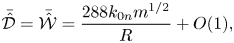 \begin{equation} \bar{\hat{\mathcal{D}}} =\bar{\hat{\mathcal{W}}}= \frac{288 k_{0n} m^{1/2}}{R} + O(1), \end{equation}
which is plotted in figure 3(c), showing excellent agreement with the numerical calculation.
Note that although asymptotically large values of  $m$ are not feasible for conventional materials, the scalings show reasonable agreement with the numerical simulations even for $O(1)$ values of the wall mass (figure 3) and so this analysis provides insight into the mechanism of TWF in feasible parameter regimes. At leading order the oscillating wall and the fluid are perfectly in phase ( $\phi$ is purely real when normalised by $\eta$), where the net work done by the fluid stress on the wall releases energy ( $\bar {\hat {\mathcal {W}}}>0$) which is then dissipated by viscous effects across the boundary layer beneath the wall ( $\bar {\hat {\mathcal {D}}}>0$). The neutrally stable TWF oscillation results in a slightly less negative (steady) pressure gradient along the channel compared with the baseline flow ( $\overline {{\breve p}_x}>0$), but the accompanying decrease in energy is a higher-order effect i.e. the work done by Reynolds stresses does not feature at leading order in the energy balance. This observation contrasts with the TWF modes of Lebbal et al. (Reference Lebbal, Alizard and Pier2022), who found TWF modes driven by the working of Reynolds stresses, although the rate of working of fluid normal stress on the wall is also a (less significant) source of energy.
3.3.1. The limit of large wall mass and Reynolds number
The scalings identified above assume that the Reynolds number remains  $O(1)$ with respect to the increasing wall mass. However, we note that the neutral stability curves in figure 2 indicate a different scaling regime for larger Reynolds numbers, where the critical wavenumber (figure 2a) and frequency both increase weakly with $R^{1/16}$, while the critical wavespeed is independent of Reynolds number (figure 2b). In principle, the scalings (3.1) could be modified to capture this behaviour by setting $R=R_0 m^n$, for some $n>0$. In this case the leading-order dispersion relation would again be (3.1f) with corresponding critical wavespeed $c_n = \sqrt {T/m}$. This approximation is plotted as open circles in figure 2(b), showing excellent agreement with the neutral stability curves for large Reynolds numbers. Setting $n=1$ would balance the convective inertia with the viscous dissipation at leading order across the boundary layer. However, if $n>1$ then the boundary layer profile for neutrally stable TWF can be further decomposed into distinct layers including a viscous layer adjacent to the wall, an inviscid shear layer and a critical layer (similar to the ‘triple-deck’ decomposition of neutrally stable TWF arising in Blasius flow over a compliant surface discussed by Carpenter & Gajjar Reference Carpenter and Gajjar1990); a typical example of the eigenfunction profile in this regime is shown in figure 5. The neutral stability curves in figure 2(a) suggest that this new scaling regime emerges for $n \approx 2$, while consistency with the observed scaling in Reynolds number would suggest $n \approx 8$. However, we do not pursue this scaling further here.
4. Stability of Poiseuille flow including wall damping
We now consider the additional influence of wall damping on the stability of the flexible-walled system. In particular, we trace the neutral stability curves of TWF and SD numerically (§ 4.1), construct an asymptotic approximation to these neutral stability curves in the limit of large wall damping (§ 4.2) and examine mode interactions with the hydrodynamic modes for large wall mass (§ 4.3).
4.1. Numerical results
We consider the numerical results in two stages. First, we consider weak damping (§ 4.1.1) to examine how the class B TWF modes from § 3 are perturbed by an irreversible energy transfer to the wall. We then consider large wall damping (§ 4.1.2), where unstable SD modes destabilise for much lower Reynolds numbers and rearrange the structure of the neutral stability curves.
4.1.1. Weak wall damping
To examine the influence of weak wall damping on the TWF normal mode of § 3.1, figure 6 illustrates the TWF neutral stability curves as the wall damping is increased from low values, showing the critical wavenumber (figure 6a) and the critical frequency (figure 6b) as a function of the Reynolds number. TWF is stabilised by wall damping (as expected), where the critical wavenumber and frequency are both reduced for all values of the Reynolds number; the short-wavelength scaling of the neutral stability curve for large Reynolds numbers is overwhelmed by even small amounts of damping (see curve for  $d=0.25$), with the critical wavenumber decreasing weakly with $R$ for finite damping.
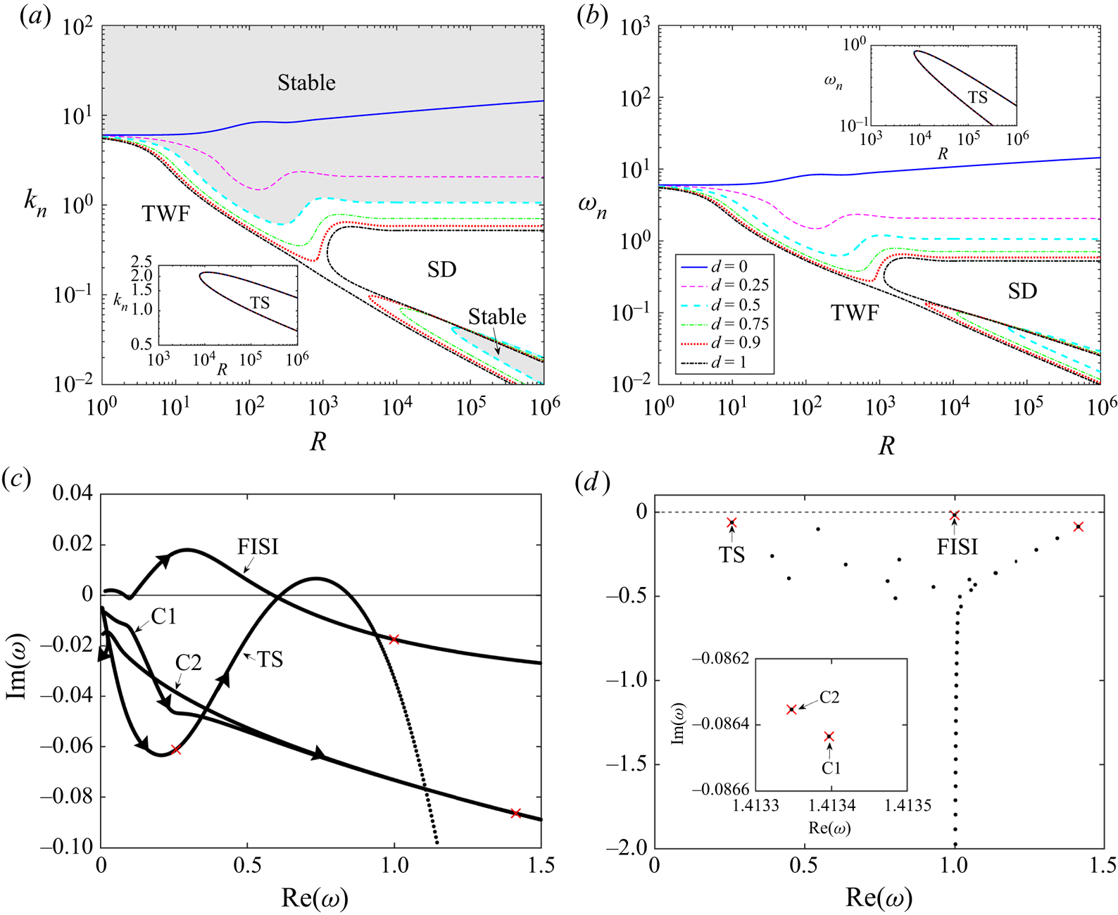
Figure 6. Neutrally stable curves of Poiseuille flow as a function of Reynolds number for various small values of the wall damping with fixed wall mass ( $m=10$) and pre-tension ( $T=10$) illustrating: (a) the critical wavenumber $k_n$ ; (b) the critical frequency $\omega _n$. In each panel we consider $d=0$ (solid line), $d=0.25$ (dashed line), $d=0.5$ (dashed line), $d=0.75$ (dash-dotted line), $d=0.9$ (dotted line) and $d=1$ (dash-dotted line). The shaded regions in (a) indicate where the base state is asymptotically stable for $d=0.5$. The insets indicate the neutral stability curves traced as a function of $R$ for the TS mode in terms of (a) critical wavenumber, (b) critical frequency. Normal modes of the weakly damped system including: (c) trace of the five most unstable eigenvalues in the complex frequency plane as a function of wavenumber for $R=10\ 000$ and $d=0.9$, where arrows indicate the direction of increasing wavenumber and red crosses indicate eigenvalues for $k=1$; (d) wider eigenvalue spectrum for $k=1$ and $R=10\ 000$, with an inset around the two most unstable centre modes.
As the wall damping increases a second neutral stability curve also becomes evident (see figure 6 for  $d=0.5$, $d=0.75$, $d=0.9$), encompassing a stable island within the TWF unstable region. As the wavenumber increases, the locus of the surface-based mode in the complex frequency plane is deviated toward the locus of another hydrodynamic mode (figure 6c), causing it to cross into the lower half-plane and form a stable zone. We identify this hydrodynamic mode by continuing to larger wavenumbers, showing that it takes the form of a ‘centre’ mode, located on the P branch of the eigenvalue spectrum with wavespeed close to the maximal flow speed (Schmid & Henningson Reference Schmid and Henningson2001); see the corresponding eigenvalue spectrum in figure 6(d). Such centre modes have recently been identified as destabilising in channel flows of viscoelastic fluids (Khalid et al. Reference Khalid, Chaudhary, Garg, Shankar and Subramanian2021), but this mode always remains stable in the present case. This stable island enlarges as the wall damping increases, where the encompassing neutral stability curve interacts with the outer TWF neutral stability curve, deviating toward one another (e.g. see neutral stability curves for $d=0.9$ in figure 6a,b). For sufficiently large wall damping this stable loop interacts with the TWF neutral curve, merging and separating in a different configuration (see curves for $d=1$ in figure 6a,b); this neutral curve structure is discussed in greater detail in § 4.1.2. Note that the neutral stability curves for TS (insets to figure 6a,b) are not significantly influenced by wall damping. In summary, this figure demonstrates that neutrally stable TWF is stabilised by wall damping, reducing the critical wavenumber but also facilitating a mode interaction which creates a stable island within the TWF unstable region. Furthermore, figure 6 shows how the three neutrally stable points for a given Reynolds number (for sufficiently large wall damping) all arise from instability of the same normal mode.
4.1.2. Large wall damping
To examine the stability of the system for values of the wall damping beyond the merger noted previously, figure 7 illustrates the neutral stability curves as a function of Reynolds number in terms of the critical wavenumber (figure 7a) and the critical frequency (figure 7b). The neutral stability curves are rearranged compared with figure 6: the low Reynolds number portion of the TWF neutral curve has merged with the lower branch of the stable loop, forming a single neutral stability curve for TWF, while the large-Reynolds-number portion of the TWF neutral stability curve has merged with the upper branch of the stable loop forming a two branch loop for class A SD. Hence, similar to Stewart et al. (Reference Stewart, Waters and Jensen2010b), SD is only unstable above a critical Reynolds number and the neutral stability curve exhibits a two branch structure; we term the upper (lower) branch as that with greater (lower) critical wavenumber. For non-zero wall damping the time-averaged work done by the fluid normal stress on the wall ( $\bar {\hat {\mathcal {W}}}$) is always positive for all normal modes (figure 7c). We note that along the upper branch of the SD neutral stability curve the activation energy is weakly negative (figure 7d), approaching zero from below as the Reynolds number increases. This suggests that the upper branch SD for large damping is nearly class C, reminiscent of the class C divergence mode that becomes unstable in damped potential flow (Appendix A). However, we show in § 4.2 that this upper-branch neutral stability curve approaches zero wavenumber as the Reynolds number increases, and so the critical wavenumber does not asymptote to $k_d$ as $R \rightarrow \infty$. We also show below that this upper-branch SD mode exhibits a very different energy balance to the inviscid divergence mode, involving viscous effects at leading order, and so we cannot conclude that these two modes are aligned.
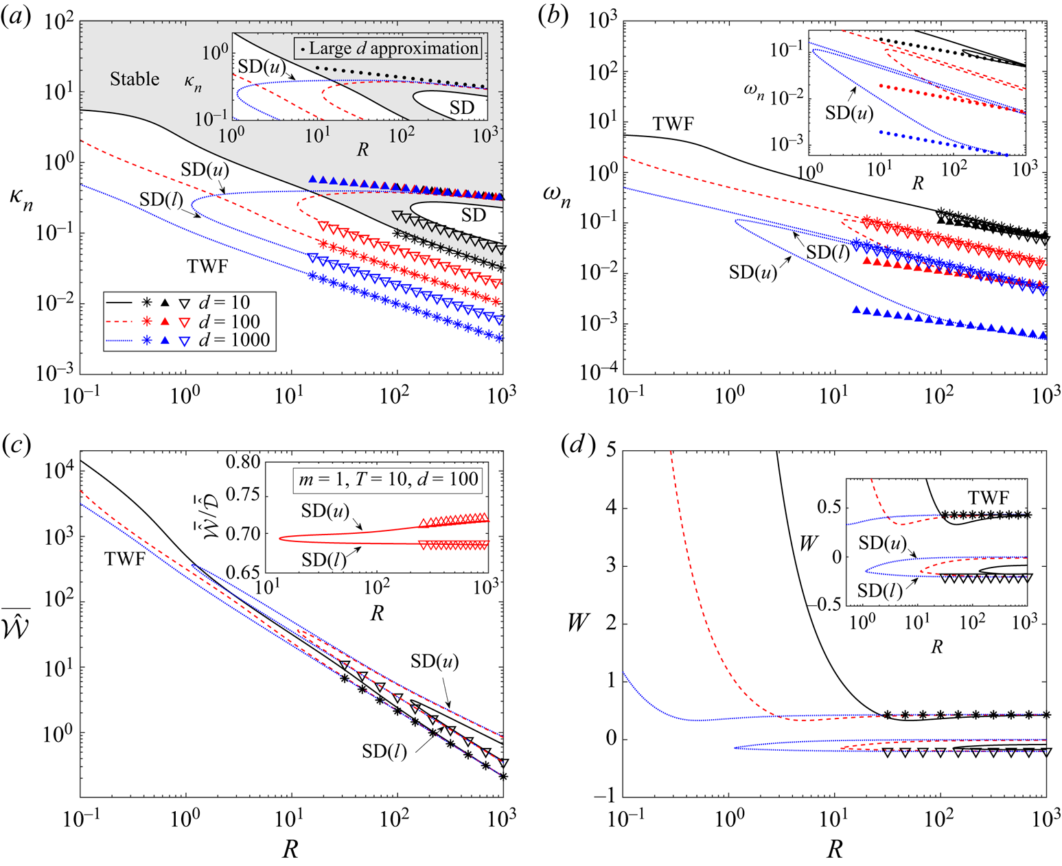
Figure 7. Neutral stability curves of Poiseuille flow as a function of Reynolds number for various large values of the wall damping with fixed wall mass ( $m=10$) and pre-tension ( $T=10$), illustrating: (a) the critical wavenumber $k_n$; (b) the critical frequency $\omega _n$; (c) the negative of the work done by the fluid stress on the wall $\bar {\hat {\mathcal {E}}}=-\bar {\hat {\mathcal {W}}}$; (d) the activation energy $W$. In each panel we consider $d=10$ (black), $d=100$ (red) and $d=1000$ (blue). The shaded region in (a) indicates where the base state is asymptotically stable for $d=10$. The symbols in (a), (b) and (d) correspond to the leading-order prediction of the large $d$ approximation for TWF (asterisks, (4.13a,b) with $+$), SD(l) (filled triangles, (4.13a,b) with $-$) and SD(u) (open inverted triangles, (4.38a,b)). The insets in (a) and (b) show the neutral stability curves as a function of Reynolds number for the large $d$ theory (filled circles, (4.37a,b)). The inset to (c) shows the ratio of the work done by fluid normal stress on the wall ( $\bar {\hat {\mathcal {W}}}$) to the energy dissipation in the bulk fluid ( $\bar {\hat {\mathcal {D}}}$) computed numerically for SD as a function of Reynolds number, alongside asymptotic predictions in the limit of large damping for both lower-branch SD (inverted triangles, computed from (4.16)) and upper-branch SD (triangles, computed numerically from (4.19)). The inset in (d) shows a close-up around zero activation energy.
In order to assess the properties of these FISI, figure 8 plots neutral stability curves of the system as a function of wall damping. As expected, for each Reynolds number the system exhibits three neutral stability curves for sufficiently large wall damping; the neutral stability curves for TWF and lower branch SD are parallel and exhibit similar critical wavenumber (figure 8a) and frequency (figure 8b), where both scale with  $d^{-1/2}$ as $d\rightarrow \infty$. Conversely, upper-branch SD exhibits critical wavenumber independent of wall damping (figure 8a) and the critical frequency scales with $d^{-1}$ as $d \rightarrow \infty$ (figure 8b). We utilise these scalings in § 4.2 to construct rational asymptotic descriptions of TWF and SD in the limit of large wall damping.
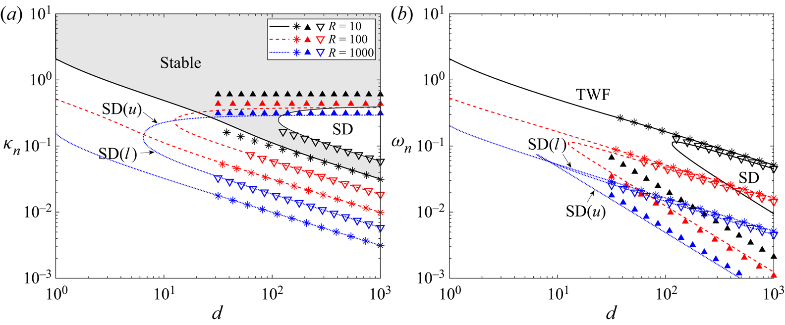
Figure 8. Neutral stability curves of Poiseuille flow as a function of the wall damping for various Reynolds numbers with fixed wall mass ( $m=10$) and pre-tension ( $T=10$), illustrating: (a) the critical wavenumber $k_n$; (b) the critical frequency $\omega _n$. In each panel we consider $R=10$ (black), $R=100$ (red) and $R=1000$ (blue). The shaded region in (a) indicates where the base state is asymptotically stable for $R=10$. The symbols correspond to the leading-order prediction of the large $d$ approximation for TWF (asterisks, (4.13a,b) with $+$), SD(l) (filled triangles, (4.13a,b) with $-$) and SD(u) (open inverted triangles, (4.38a,b)).
To elucidate the spatial structure of the three neutrally stable FISI, figure 9 illustrates the streamfunction profiles of TWF (figure 9a), lower-branch SD (figure 9b) and upper-branch SD (figure 9c) for the same Reynolds number and choice of wall properties. The spatial profiles of TWF and lower-branch SD are similar, exhibiting a non-trivial asymmetric profile across the entire domain. Conversely, upper-branch SD exhibits rapid variations across narrow boundary layers adjacent to the channel walls, indicating a substantial difference in mechanism.
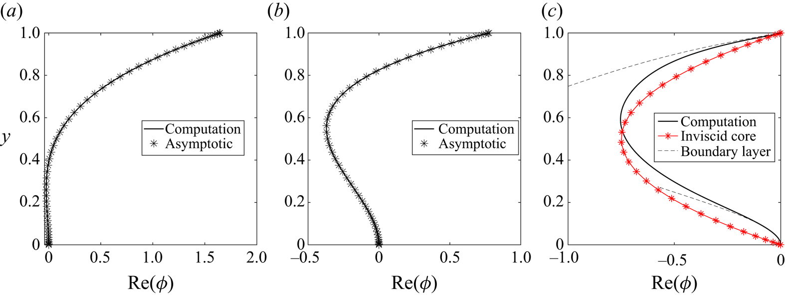
Figure 9. Neutrally stable eigenfunctions  $\phi$ for (a) TWF; (b) SD(l); (c) SD(u). The asterisks in (a,b) correspond to the leading-order asymptotic prediction for large wall damping (4.6). The asterisks in (c) correspond to the inviscid core solution (4.22), while the dashed lines correspond to the two boundary layer solutions (4.26) and (4.30). Here, $T=10$, $m=10$ and $R=1000$.
4.2. The limit of large wall damping
The scalings identified in § 4.1 facilitate a rational asymptotic description of neutrally stable TWF and SD modes in the limit of large wall damping, building on the ad hoc description of lower-branch SD provided by Stewart et al. (Reference Stewart, Waters and Jensen2010b) (based on a flow profile assumption). In particular, in the limit of large wall damping we describe neutrally stable lower-branch SD and TWF (§ 4.2.1) and neutrally stable upper-branch SD (§ 4.2.2).
4.2.1. Neutrally stable TWF and lower-branch SD in the limit of large wall damping
Following the scalings identified in § 4.1 we return to the inhomogeneous system (2.11) and treat the wall damping as a large parameter ( $d\gg 1$). We adopt a long-wavelength, low-frequency rescaling in the form
 \begin{equation} k = d^{{-}1/2} k_0, \quad \omega = d^{{-}1/2} \omega_0 + d^{{-}1} \omega_1 + O(d^{{-}3/2}), \end{equation}
where  $k_0$ and $\omega _0$ are to be determined at neutral stability. We expand the perturbation streamfunction and the dispersion relation $D$ according to
 \begin{equation} \phi = \phi_0 + d^{{-}1/2} \phi_1 + O(d^{{-}1}), \quad D=d^{1/2} D_0 + D_1 + O(d^{{-}1/2}). \end{equation}
The inhomogeneous Orr–Sommerfeld system (2.11) becomes at leading order
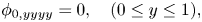 \begin{equation} \phi_{0,yyyy}=0, \quad (0\le y \le 1), \end{equation}
subject to boundary conditions
 \begin{gather} \phi_0=0, \quad \phi_{0,y}=0 \quad (y=0), \end{gather}
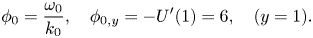 \begin{gather}\phi_0=\frac{\omega_0}{k_0}, \quad \phi_{0,y}={-}U'(1) = 6, \quad (y=1). \end{gather}
We solve for  $\phi _0$ explicitly in the form
 \begin{equation} \phi_0(y) = \frac{1}{k_0}y^2(\omega_0 (3 - 2y) + 6 k_0 ({-}1 + y)), \quad (0\le y \le 1). \end{equation}
Given  $k_0$ and $\omega _0$ as calculated below, this profile is plotted in figure 9(a) (figure 9(b)) against numerical predictions of the eigenfunction for TWF (lower-branch SD) showing excellent agreement. In both cases the leading-order streamfunction is purely real for neutrally stable solutions.
Substituting these expansions into the normal stress balance (2.11d) and substituting for  $\phi _0$ we obtain the leading-order dispersion relation
 \begin{equation} D_0(\omega_0,k_0) \equiv \frac{1}{ik_0 R}\phi_{0,yyy}(1) + i\omega_0 = \frac{12}{ik_0 R}\left(\frac{3\omega_0}{k_0}-1\right) + i\omega_0, \end{equation}
where the first term corresponds to viscous effects and the second term is due to wall damping. For normal modes  $D_0(\omega _0,k_0)=0$, so we have
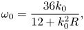 \begin{equation} \omega_0= \frac{36 k_0}{12 + k_0^2 R}, \end{equation}
where  $\omega _0$ is purely real for $k_0$ real.
To fix the corresponding critical wavenumber of the system we expand the governing equations to the following order in the form:
 \begin{equation} \frac{1}{ik_0 R}{\phi}_{1,yyyy} = \left(U - \frac{\omega_0}{k_0}\right) {\phi}_{0,yy} -U_{yy}{\phi}_0, \end{equation}
subject to the inhomogeneous boundary conditions
 \begin{gather} {\phi}_1(0)=0, \quad {\phi_{1,y}}(0)=0, \end{gather}
 \begin{gather}{\phi}_1(1)=\frac{\omega_1}{k_0}, \quad {\phi_{1,y}}(1)=0. \end{gather}
We integrate (4.9) four times and apply the four boundary conditions to determine  $\phi _1$ explicitly as a polynomial in $y$. The normal stress condition (2.11d) at $O(1)$ then implies the first-order correction to the dispersion relation, in the form
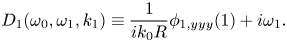 \begin{equation} D_1(\omega_0,\omega_1,k_1) \equiv \frac{1}{i k_0 R}\phi_{1,yyy}(1) + i\omega_1. \end{equation}
Setting  $D_1=0$ and substituting for $\phi _1(y)$, we obtain the correction to the frequency in the form
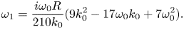 \begin{equation} \omega_1 = \frac{i \omega_0 R}{210 k_0}(9k_0^2 - 17\omega_0 k_0 + 7 \omega_0^2 ). \end{equation}
Looking for neutrally stable solutions ( ${\rm Im} (\omega _1)=0$), we obtain a second constraint linking $k_0$ and $\omega _0$ in the form
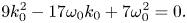 \begin{equation} 9k_0^2 - 17\omega_0 k_0 + 7 \omega_0^2=0. \end{equation}
Solving the constraints (4.8) and (4.12) simultaneously, we obtain a pair of physical solutions which can be rewritten in terms of the unscaled dimensionless variables and parameters in the form
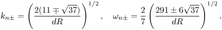 \begin{equation} k_{n\pm} = \left(\frac{2(11 \mp \sqrt{37})}{dR} \right)^{1/2}, \quad \omega_{n\pm} = \frac{2}{7}\left(\frac{291\pm 6 \sqrt{37}}{dR} \right)^{1/2}. \end{equation}
These solutions are almost indistinguishable from the numerically computed neutral stability curves as  $d$ becomes large (figures 7a,b and 8a,b), where $k_{n+}$ corresponds to TWF and $k_{n-}$ corresponds to lower-branch SD.
The dispersion relation (2.11d) expanded to first order ( $D\approx d^{1/2}D_0+D_1$) can be differentiated to calculate the leading-order activation energy (2.18). Applying the neutral stability condition (4.8), the corresponding activation energy can be calculated as
 \begin{equation} {{W}}_\pm = {\frac{3 (37 \pm 17 \sqrt{37})}{980}} + O(d^{{-}1/2}), \end{equation}
independent of Reynolds number. So neutrally stable TWF (SD), the  $+(-)$ branch of solutions, has positive (negative) activation energy, as expected. Again these show excellent agreement with numerically computed activation energy along the two neutrally stable branches (figure 7d).
This asymptotic analysis elucidates the steady correction to driving pressure gradient (2.13), which can be calculated as
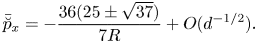 \begin{equation} \bar{\breve p}_x ={-}\frac{36(25 \pm \sqrt{37})}{7R} + O(d^{{-}1/2}). \end{equation}
Hence, unlike TWF modes described in the limit of large mass (§ 3.3), the oscillating flow serves to make the steady pressure gradient along the channel more negative at leading order.
Furthermore, we calculate the leading-order contributions to the terms in the time-averaged energy budget (2.17), where we obtain
 \begin{equation} (\bar{\hat{\mathcal{D}}},\bar{\hat{\mathcal{W}}},\bar{\hat{\mathcal{P}}})=\frac{(25\pm\sqrt{37})}{49R}(804,552,252) +O(d^{{-}1/2}). \end{equation}
Hence, approximately 2/3 of the energy consumed by dissipation across the bulk ( $\bar {\hat {\mathcal {D}}}$) is provided by the working of fluid stresses on the wall ( $\bar {\hat {\mathcal {W}}}$), in strong agreement with the numerical simulations (inset to figure 7c), with the remaining amount released by a decrease in the steady (negative) pressure gradient along the channel ( $\bar {\hat {\mathcal {P}}}$). However, in this case we also note that the contributions involving breved variables to the leading-order terms in the time-averaged energy budget (2.17) combine perfectly to zero at this order, and so there is an additional balance between the terms involving hatted variables in $\bar {\hat {\mathcal {W}}}$ and $\bar {\hat {\mathcal {D}}}$, suggesting a similar mechanism to the TWF mode described in § 3.3 where the correction to the mean flow does not play a role; this balance is not true in general and arises because the leading-order eigenfunction is purely real when normalised on the wall deflection, so the wall and flow are perfectly in phase at neutral stability.
Note that, although asymptotically large values of wall damping are not feasible for conventional materials, the scalings show reasonable agreement with the numerical simulations even for  $O(1)$ values (figure 8) and so this analysis provides insight into the mechanism of these FISI in feasible parameter regimes. At leading order the oscillating wall and the fluid are perfectly in phase ( $\phi$ is purely real when normalised by $\eta$), where both the net work done by the fluid stress on the wall ( $\bar {\hat {\mathcal {W}}}>0$) and the work done by the steady pressure gradient ( $\bar {\hat {\mathcal {P}}}>0$) release energy (in a ratio of approximately 2 : 1), which is then dissipated by viscous effects across the channel ( $\bar {\hat {\mathcal {D}}}>0$). A similar mechanism of SD driven by the working of fluid normal stress on the wall was recently noted by Lebbal et al. (Reference Lebbal, Alizard and Pier2022). However, their work found that TWF modes were primarily driven by the rate of working of Reynolds stresses, in contrast to the modes analysed here, although the working of fluid normal stress on the wall was also shown to be mildly destabilising.
4.2.2. Neutrally stable upper-branch SD in the limit of large wall damping
Following the scalings identified in figure 8 we return to the full model (2.11) and assume the wavenumber remains  $O(1)$ with respect to the wall damping and rescale according to
 \begin{equation} k=k_0, \quad \omega = d^{{-}1} \omega_0 + O(d^{{-}2}), \end{equation}
where we calculate the criticality conditions in terms of the wavenumber  $k_0$ and leading-order frequency $\omega _0$. Similarly, we expand the streamfunction according to
 \begin{equation} \phi = \phi_0 + O(d^{{-}1}). \end{equation}
The inhomogeneous linear stability problem (2.11) becomes at leading order
 \begin{equation} U (\phi_{0,yy} - k_0^2 \phi_0) - U_{yy}\phi_0 = \frac{1}{i k_0 R}(\phi_{0,yyyy} - 2k_0^2 \phi_{0,yy}+ k_0^4 \phi_0), \end{equation}
subject to boundary conditions
 \begin{gather} \phi_0=0, \quad \phi_{0,y}=0 \quad (y=0), \end{gather}
 \begin{gather}\phi_0=0, \quad \phi_{0,y}={-}U_y(1) = 6, \quad (y=1); \end{gather}
note that the leading-order kinematic boundary condition does not involve the wall profile in this limit. This system for  $\phi _0$ is notably independent of the leading-order frequency $\omega _0$. Substituting these expansions into the normal stress balance (2.11d) leads to the dispersion relation
 \begin{equation} D(\omega_0,k_0) \equiv \frac{1}{ik_0 R}({\phi}_{0,yyy}(1) - k_0^2 \phi_{0,y}(1) ) - T k_0^2 + i \omega_0 + O(d^{{-}1}). \end{equation}
In this case, the wall mass does not feature in the leading-order problem, but, unlike lower-branch SD modes (§ 4.2.1), the restoring force due to wall tension features prominently. To the best of our knowledge it is not possible to solve this system analytically, but numerical solution is straightforward using a spectral method analogous to that described in § 2.4. It emerges that numerical solution of the leading-order system (4.19) is sufficient to isolate the critical conditions for instability; these neutral stability curves are shown in figure 7, plotting the approximated critical wavenumber (inset to figure 7a) and critical frequency (inset to figure 7b) as a function of the Reynolds number, showing excellent agreement with the numerically computed neutral stability curves of upper-branch SD.
Given the leading-order dispersion relation (4.19d) we find that the leading-order activation energy for neutrally stable upper branch SD is  $O(d^{-1})$ and so approaches zero as the wall damping becomes large, consistent with the numerical simulations (figure 8d). Hence, this upper-branch SD mode approaches class C as the wall damping becomes large, reminiscent of the inviscid divergence mode (Appendix A).
This approach does not provide analytical insight into the partition of energy, but we note that numerical calculation of the corresponding energy terms in (2.17), plotted as symbols in figure 7(c), show excellent agreement with the full computations. These numerical computations indicate that the mechanism of upper-branch SD is broadly similar to lower-branch SD, with energy released by the working of fluid stress on the wall ( $\bar {\hat {\mathcal {W}}}>0$) and the working of the steady pressure gradient along the channel ( $\bar {\hat {\mathcal {P}}}$), which is then dissipated by viscous effects across the bulk ( $\bar {\hat {\mathcal {D}}}$). In the limit of large damping the ratio of work done by fluid normal stress on the wall compared with the work done by dissipation in the fluid $\bar {\hat {\mathcal {W}}}/\bar {\hat {\mathcal {D}}} \approx 0.73$ as $R \rightarrow \infty$ (almost perfectly independent of $T$); this value is close to, but slightly larger than, that predicted for lower-branch SD ( $\bar {\hat {\mathcal {W}}}/\bar {\hat {\mathcal {D}}} = 46/67 \approx 0.69$, § 4.2.1), but the balance is broadly similar. Interestingly, unlike lower-branch SD, the contributions to these energies which arise from the (breved) terms do not all cancel internally, and so contribute to the overall partition (the leading-order eigenfunction is complex, so the wall and streamfunction profiles are not in phase, and the work done by Reynolds stresses is non-negligible).
To form a more intuitive description of the flow we consider the leading-order system in the limit of large damping (4.19) in the additional limit of large Reynolds number. It emerges that the eigenfunction  $\phi _0$ can be separated into an inviscid core with viscous effects confined to a narrow boundary (critical) layers adjacent to the walls. Based on the scalings evident in figure 7(a,b), we consider long-wavelength, low-frequency instabilities of the form
 \begin{equation} k_0 = R^{{-}1/7} k_{00}, \quad \omega_0 = R^{{-}2/7} \omega_{00} + O(R^{{-}4/7}). \end{equation}
 Across the inviscid core, the eigenfunction  $\phi _0$ is expanded according to
 \begin{equation} \phi_0 = \phi_{00} + R^{{-}2/7} \phi_{01} + O(R^{{-}4/7}), \end{equation}
where the governing equations (4.19) become at leading order in  $R$
$R$
 \begin{equation} U\phi_{00,yy} - U_{yy}\phi_{00} = 0, \end{equation}
subject to reduced boundary conditions
 \begin{equation} \phi_{00}(0)=0, \quad \phi_{00}(1)=0. \end{equation}
This system admits the simple solution  $\phi _{00} = A U$, where $A$ is an undetermined constant. Note that this inhomogeneous system has already been normalised with respect to the wall deflection, and so $A$ must be calculated as part of the solution. Plotting this parabolic profile (for $A$ as computed below) shows reasonable agreement with the numerically computed eigenfunction (figure 9c). In this case the outer limit of the axial velocity component takes the form
 \begin{gather} \phi_{00,y} \rightarrow A U_y(0) = 6A \ \text{as} \ y\rightarrow 0, \end{gather}
 \begin{gather}\phi_{00,y} \rightarrow A U_y(1) ={-}6A \ \text{as} \ y\rightarrow 1. \end{gather}
 For large Reynolds numbers the flow exhibits narrow boundary layers adjacent to the walls of width  $R^{-2/7}$. Adjacent to the rigid wall (denoted with the superscript $^{(r)}$) we rescale
 \begin{equation} y=R^{{-}2/7} Y, \quad \phi_0 = R^{{-}2/7} \varPhi^{(r)}_{00}(Y) + O(R^{{-}4/7}). \end{equation}
In this case, the governing equations (4.19) take the leading-order form across the boundary layer
 \begin{equation} 6 Y k_{00} \varPhi^{(r)}_{00,YY} + i \varPhi^{(r)}_{00,YYYY} = 0, \quad (Y \ge 0), \end{equation}
subject to boundary conditions
 \begin{equation} \varPhi^{(r)}_{00}(0)=0, \quad \varPhi^{(r)}_{00,Y}(0)=0, \quad \varPhi^{(r)}_{00,Y} \rightarrow 6A \ \text{as} \ Y \rightarrow \infty. \end{equation}
This is Airy's equation in  $\varPhi ^{(r)}_{00,YY}$, with solution
 \begin{equation} \varPhi^{(r)}_{00,YY} = A_0 \text{Ai}((6ik_{00})^{1/3} Y ) + B_0 \text{Bi}((6ik_{00})^{1/3} Y ), \end{equation}
where  $\text {Ai}$ and $\text {Bi}$ are Airy functions of the first and second kinds, respectively, and $A_0$ and $B_0$ are complex constants; we immediately set $B_0=0$ to ensure the solution is bounded at $Y=0$. Integrating this expression once, and applying the no-slip and far-field conditions (4.24b) as well as known results for the integral of Airy functions (Abramowitz & Stegun Reference Abramowitz and Stegun1965), we deduce
 \begin{equation} \varPhi^{(r)}_{00,Y}(Y) = 18 A (6ik_{00})^{1/3} \int_0^Y \text{Ai}((6ik_{00})^{1/3} \zeta)\,\text{d}\zeta. \end{equation}
For  $k_{00}$ and $A$ calculated below, this profile is plotted in figure 9(c), showing good agreement with the numerically computed streamfunction profile close to the rigid wall. This expression can be integrated once more to obtain the streamfunction explicitly, although the final expression is cumbersome and not reproduced here. In the limit as $Y\rightarrow \infty$ we obtain the limiting form
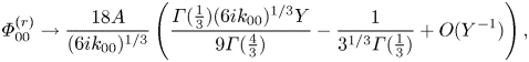 \begin{equation} \varPhi^{(r)}_{00} \rightarrow \frac{18 A}{(6ik_{00})^{1/3}}\left( \frac{\varGamma(\frac{1}{3})(6ik_{00})^{1/3}Y}{9 \varGamma(\frac{4}{3})} - \frac{1}{3^{1/3} \varGamma(\frac{1}{3})} + O(Y^{{-}1})\right), \end{equation}
where  $\varGamma ({\cdot })$ is the gamma function; this ejection of fluid from the boundary layer drives flow in the inviscid core at first-order. The leading-order fluid pressure is constant across the boundary layer on the rigid wall and takes the form
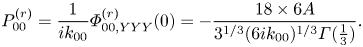 \begin{equation} P_{00}^{(r)} = \frac{1}{i k_{00}}\varPhi^{(r)}_{00,YYY}(0) ={-}\frac{18\times 6 A}{3^{1/3} (6i k_{00})^{1/3} \varGamma(\frac{1}{3})}. \end{equation}
 Similarly, adjacent to the compliant wall (denoted with the superscript  $^{(c)}$) we rescale the variables according to
 \begin{equation} y=1- R^{{-}2/7} Y, \quad \phi_0 = R^{{-}2/7} \varPhi^{(c)}_{00}(Y) + O(R^{{-}4/7}). \end{equation}
The governing equations (4.19a) across the boundary layer again reduce to Airy's equation (4.24a), subject to boundary conditions
 \begin{equation} \varPhi^{(c)}_{00}(0)=0, \quad \varPhi^{(c)}_{00,Y}(0)=U_y(1) ={-}6, \quad \varPhi^{(c)}_{00,Y} \rightarrow -A U_y(1) = 6A \ \text{as} \ Y \rightarrow \infty. \end{equation}
In a similar manner to the other boundary layer, we deduce
 \begin{equation} \varPhi^{(c)}_{00,Y}(Y) = U_y(1) + 18 (1+ A ) (6ik_{00})^{1/3} \int_0^Y \text{Ai}((6ik_{00})^{1/3} \zeta)\,\text{d}\zeta. \end{equation}
For  $k_{00}$ and $A$ calculated below, this profile is also shown in figure 9(c), again showing close agreement to the numerically computed profile close to the flexible wall. As before, this expression can be integrated once more to obtain the limiting form of the streamfunction as $Y\rightarrow \infty$ in the form
 \begin{equation} \varPhi^{(c)}_{00} \rightarrow -6Y + \frac{18 (A+1)}{(6ik_{00})^{1/3}}\left( \frac{\varGamma(\frac{1}{3}) (6ik_{00})^{1/3}Y}{9 \varGamma(\frac{4}{3})} - \frac{1}{3^{1/3} \varGamma(\frac{1}{3})} + O(Y^{{-}1})\right), \end{equation}
which, similar to the boundary layer on the rigid wall, drives flow in the inviscid core at first order. The leading-order fluid pressure is constant across the boundary layer on the compliant wall and takes the form
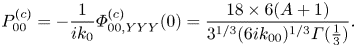 \begin{equation} P_{00}^{(c)} ={-}\frac{1}{i k_0}\varPhi^{(c)}_{00,YYY}(0) = \frac{18\times 6 (A+1)}{3^{1/3} (6 i k_{00})^{1/3} \varGamma(\frac{1}{3})}. \end{equation}
 The upper and lower boundary layer profiles can be solved for a given  $A$. To determine the constant $A$ we expand the inviscid core flow to the following order in $R^{-2/7}$ to obtain the governing equations
 \begin{equation} U\phi_{01,yy} - U_{yy}\phi_{01} = (U\phi_{01,y} - U_y \phi_{01})_y= A k_{00}^2 U^2, \end{equation}
subject to boundary conditions modified by the flow ejected from the boundary layers (4.27a), (4.31a), in the form
 \begin{equation} \phi_{01}(0)= \frac{18 A}{3^{1/3}(6ik_{00})^{1/3} \varGamma(\frac{1}{3})}, \quad \phi_{01}(1)= \frac{18 (A+1)}{3^{1/3}(6ik_{00})^{1/3}\varGamma(\frac{1}{3})}. \end{equation}
This system can be solved directly using the method of variation of parameters. However, we note that the  $x$-momentum equation (2.6a) expanded to $O(R^{-2/7})$ across the inviscid core can be expressed as
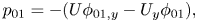 \begin{equation} p_{01} ={-}(U\phi_{01,y} - U_y \phi_{01}), \end{equation}
so that (4.32a) can be written in terms of the fluid pressure, in the form
 \begin{equation} p_{01,y} ={-}A k_{00}^2 U^2. \end{equation}
Furthermore, using (4.33), the boundary conditions on  $\phi _{01}$ (4.32b) can be re-written in terms of the fluid pressure in the lower (4.27b) and upper boundary layers (4.31b), such that
 \begin{equation} p_{01}(0) = P_{00}^{(r)} ={-}\frac{18\times 6 A}{3^{1/3} (6i k_{00})^{1/3} \varGamma(\frac{1}{3})}, \quad p_{01}(1) = P_{00}^{(c)} = \frac{18\times 6 (A+1)}{3^{1/3} (6 i k_{00})^{1/3} \varGamma(\frac{1}{3})}. \end{equation}
The two boundary layers are interacting across the core flow, in a similar manner to the large-Reynolds-number approximation to lower-branch TS instabilities in a rigid channel (Bogdanova & Ryzhov Reference Bogdanova and Ryzhov1983; Pedley Reference Pedley2000; Stewart et al. Reference Stewart, Waters and Jensen2010b). Integrating (4.34a) once and applying both boundary conditions (4.34b), determines the amplitude of the leading-order flow in the inviscid core, in the form
 \begin{equation} A=\left({-}2 + \frac{6}{5}k_{00}^2\frac{3^{1/3} (6ik_{00})^{1/3} \varGamma(\frac{1}{3})}{108} \right)^{{-}1}. \end{equation}
We note that for  $k_{00}\ll 1$ in (4.34a), where the cross-stream pressure gradient is weak, $P_{00}^{(r)}=P_{00}^{(c)}$ and this constraint reduces to $A=-\frac {1}{2}$.
The compliant wall boundary layer is coupled to the leading-order dispersion relation
 \begin{equation} D_1(\omega_{01},k_{00})\equiv P_{00}^{(c)} - T k_{00}^2 + i\omega_{00} = \frac{108 (A+1)}{3^{1/3} (6i k_{00})^{1/3} \varGamma(\frac{1}{3})} - T k_{00}^2 + i\omega_{00}. \end{equation}
Neutrally stable modes ( ${\rm Im} (\omega _{00})=0$) can be identified by setting $D_1=0$ coupled to the criterion for $A$ (4.35), resulting in a polynomial dispersion relation which can be solved for $k_{00n}$ and $\omega _{00n}$ by separating into real and imaginary parts; however, this final step must be taken numerically. In the simplified case where the cross-stream pressure gradient is weak we can approximate $A\approx -\frac {1}{2}$, these criticality conditions reduce to the explicit form
 \begin{equation} k_{00n} = \left(\frac{3^{17/6}}{2^{1/3} T \varGamma(\frac{1}{3})} \right)^{3/7} , \quad \omega_{00n}=\frac{1}{3^{1/2}}T k_{00n}^2. \end{equation}
Furthermore, these criticality conditions can be expressed in terms of the unscaled dimensionless variables and parameters in the form
 \begin{equation} k_{n} = \left(\frac{3^{17/6}}{2^{1/3} \varGamma(\frac{1}{3})} \right)^{3/7} T^{{-}3/7} R^{{-}1/7}, \quad \omega_{n}=\left(\frac{3^{9/4}}{2^{1/3} \varGamma(\frac{1}{3})} \right)^{6/7} T^{1/7} d^{{-}1} R^{{-}2/7}. \end{equation}
These expressions demonstrate excellent agreement with the numerically computed neutral stability curves shown in figures 7 and 8.
Note that this analytical calculation could be extended to explicitly compute the partition of energies for the neutrally stable modes (similar to lower-branch TWF and SD), where each term is formally  $O(R^{-1})$. However, this calculation requires the first correction to the streamfunction across the viscous boundary layers, and so is not pursued further here.
4.3. Mode interaction with TS for large wall mass
In § 3.2 we elucidated a mode interaction between the undamped TWF and TS modes for increasing wall mass, exhibiting a new stable island within the unstable TWF zone. To explore this mode interaction in the presence of wall damping, in figure 10 we plot the critical wavenumber (figure 10a) and frequency (figure 10b) of the system as a function of Reynolds number for several values of the wall mass holding all other parameters fixed. For low wall mass (e.g.  $m=10$ in figure 10), the wall damping is sufficiently large so that the SD neutral curve has disconnected from the TWF neutral curve (cf. § 4.2). As the wall mass increases the interaction with the centre mode, which leads to the separate TWF and SD neutral stability curves (§ 4.1), becomes weaker, meaning that the locus of the surface-based mode as a function of wavenumber no longer transiently crosses into the lower half-plane. Instead, the system exhibits a single neutral stability curve and the SD and TWF neutral curves merge together ( $m=100$ in figure 10). As the wall mass increases the TS and TWF modes interact and eventually merge into a configuration reminiscent of the case with low wall damping, where the system exhibits a stable loop within the outer unstable region (e.g. $m=200$). For even larger values of the wall mass the neutral stability curve self-intersects, creating a second stable island in the parameter space (e.g. $m=1000$). Hence, although increasing wall mass is destabilising to TWF, mode interaction leads to new stable islands within the unstable region. Figure 10 also exhibits further evidence of mode interaction with a visible modification to the TS neutral stability curve for large wall mass (e.g. $m\geqslant 100$). However, given that this interaction occurs for very large Reynolds numbers we do not consider this further.
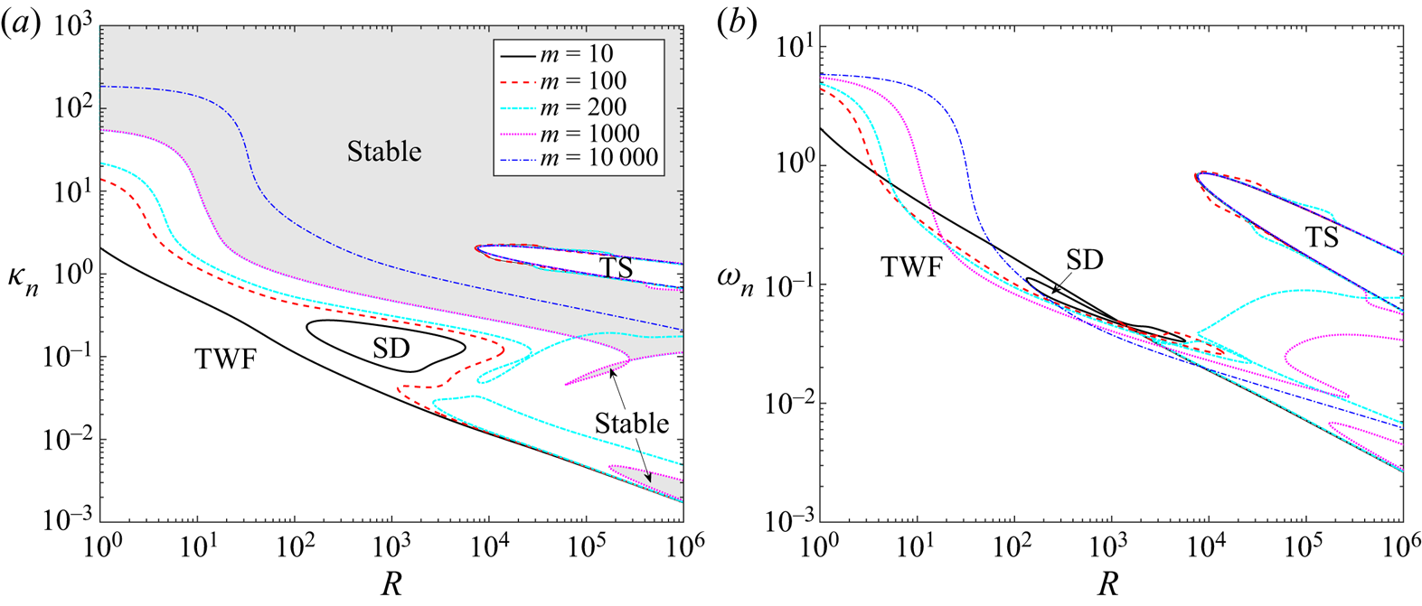
Figure 10. Neutral stability curves for Poiseuille flow as a function of wall mass for various Reynolds numbers with fixed wall damping ( $d=10$) and pre-tension ( $T=10$), illustrating: (a) the critical wavenumber $k_n$; (b) critical frequency $\omega _n$. Here, we consider $m=10$ (solid line), $m=100$ (dashed line), $m=200$ (dash-dotted line), $m=1000$ (dotted line) and $m=10\ 000$ (dash-dotted line). The shaded regions in (a) indicate where the base state is asymptotically stable for $m=1000$.
5. Discussion
In this paper we considered the stability of flow through an asymmetric collapsible channel formed by a rigid wall and a damped, tensioned wall with finite mass, considering both potential flow (with a plug profile) and viscous flow (with a fully developed Poiseuille profile). The simplified wall model is similar to classical studies of boundary layer flow over a compliant surface (Benjamin Reference Benjamin1960; Landahl Reference Landahl1962; Benjamin Reference Benjamin1963) and in flexible-walled channels (Hains & Price Reference Hains and Price1962; Green & Ellen Reference Green and Ellen1972), and is prototypical of compliant coatings used in an effort to delay laminar–turbulent transition. This choice of wall model neglects the effect of bending stiffness and spring foundation from the general formulation of a linear Euler–Bernoulli beam (these extra effects have been previously considered in other studies, see Carpenter & Garrad Reference Carpenter and Garrad1986; Davies & Carpenter Reference Davies and Carpenter1997a), in an effort to reduce the number of model parameters.
In line with previous studies of flow over a compliant surface (Carpenter & Garrad Reference Carpenter and Garrad1985, Reference Carpenter and Garrad1986) and in compliant channels (Davies & Carpenter Reference Davies and Carpenter1997a; Stewart et al. Reference Stewart, Waters and Jensen2010b), we identified several forms of instability using a combination of numerical and asymptotic analyses (in the limits of large wall mass and wall damping), elucidated their corresponding neutral stability curves and their interaction with other normal modes. Furthermore, we extended the linear stability analysis to the following order in perturbation amplitude to construct the work done by the fluid normal stress on the wall over a period of neutrally stable oscillation ( $\bar {\hat {\mathcal {W}}}$), and devised a numerical method to construct the sign of the activation energy of these normal modes, from which they were classified as either class A, B or C according to the framework of Benjamin (Reference Benjamin1960).
The simulations we have presented are restricted to a planar channel. It should be noted that our choice of non-dimensionalisation means that the Squire transformation (Squire Reference Squire1933) cannot be directly applied, and so we are unable to make any conclusions about three-dimensional perturbations. However, we note that an alternative scheme of non-dimensionalisation (where the wall parameters are scaled differently with respect to Reynolds number) is compatible with a Squire transformation and so in that case two-dimensional perturbations are always the most unstable (Rotenberry & Saffman Reference Rotenberry and Saffman1990; Lucey & Carpenter Reference Lucey and Carpenter1995; Davies & Carpenter Reference Davies and Carpenter1997a; Lebbal et al. Reference Lebbal, Alizard and Pier2022). Three-dimensional flow also allows the possibility of more elaborate design of compliant coating which may have more optimal properties for the delay of laminar–turbulent transition (e.g. Nagy, Szabó & Paál (Reference Nagy, Szabó and Paál2022) considered a three-dimensional flow over a compliant coating which can move in the streamwise direction only, exhibiting delay in the onset of TS modes), but this level of complexity in the wall model is beyond the scope of the current study.
Uniform potential flow in the absence of wall damping exhibits two normal modes, which coalesce to form an unstable flutter mode for small wavenumbers, which is class C at onset (Carpenter & Garrad Reference Carpenter and Garrad1986); this combined mode is only unstable when the destabilising influence of the wall mass exceeds the stabilising influence of the wall tension. This coalescence is overwhelmed by viscous effects in the fluid or the wall, where the constituent normal modes are (de)stabilised and instabilities instead occur through a single normal mode of the system crossing into the upper half-frequency plane. For example, for low wavenumbers, potential flow with finite wall damping exhibits a class C divergence instability through one normal mode, which onsets with zero frequency.
The viscous system with Poiseuille flow also exhibits two surface-based normal modes, in addition to an infinite family of hydrodynamic modes analogous to those in a rigid channel (Drazin & Reid Reference Drazin and Reid1981). Only one of these hydrodynamic modes can become unstable (via the classical TS mechanism), tracing a two branch neutral stability curve for large Reynolds numbers (figures 2 and 6). However, one of the surface-based normal modes can also become unstable to a flow-induced surface instability. In the absence of wall damping this surface-based normal mode becomes unstable as long-wavelength TWF, which is class B at neutral stability; this mode persists as the wall mass becomes negligible (figure 2) and so is not directly related to the inviscid flutter mode. In the limit of large wall mass the neutrally stable TWF mode becomes increasingly short wavelength (figure 3a), where the work done by the fluid normal stress on the wall releases energy which is dissipated by the non-trivial viscous flow in the adjacent boundary layer (figure 5).
Conversely, for viscous Poiseuille flow in the presence of wall damping, the inviscid divergence instability is replaced by a small wavenumber, low-frequency SD mode which has weakly positive activation energy (class A), approaching class C in the limit of large wall damping (figures 7 and 8). In this limit the neutrally stable SD perturbation profile exhibits narrow viscous layers adjacent to the channel walls which interact across an inviscid core (figure 9c), similar to lower-branch TS instabilities (Bogdanova & Ryzhov Reference Bogdanova and Ryzhov1983). However, across the range of unstable wavenumbers the surface-based normal mode can interact with the most unstable centre mode (a stable hydrodynamic mode with wavespeed close to the maximal flow speed, Schmid & Henningson Reference Schmid and Henningson2001), partially stabilising the surface-based mode for an intermediate range of wavenumbers (figure 7). This narrow range is confined by two neutral stability curves which run parallel, the lower corresponding to a class B TWF mode and the upper to a class A SD mode (figures 7 and 8). Despite having contrasting responses to an irreversible energy transfer from the wall, these two neutrally stable modes have similar character and have been simultaneously described in the limit of large wall damping, where viscous effects are distributed across the entire channel (figure 9a,b). We note in the limit of large damping both TWF and SD exhibit a similar partition of energy at neutral stability, where approximately 2/3 of the energy dissipated by the fluid viscosity is released by the working of normal stress on the flexible wall, while the remaining 1/3 arises due to a modification to the steady pressure gradient along the channel. Note that a similar mechanism of SD, driven by the rate of working of fluid normal stress on the wall, was recently noted by Lebbal et al. (Reference Lebbal, Alizard and Pier2022).
For sufficiently large wall mass the surface-based normal modes can interact with the TS mode (even when it is stable), and the subsequent deviation of the frequency leads to stable islands within the large unstable region (figures 2, 4, 10). These stable zones enlarge with increasing wall mass, and could be of use in designing compliant coatings for delaying laminar–turbulent transition.
In this paper, focus was restricted to analysis of normal modes and their interactions. However, non-modal analysis of Poiseuille flow through rigid channels or rigid pipes has indicated that non-normality of the Orr–Sommerfeld operator can lead to substantial transient growth in regions of the parameter space where the flow is asymptotically stable (Reddy & Henningson Reference Reddy and Henningson1993; Schmid & Henningson Reference Schmid and Henningson2001; Schmid Reference Schmid2007). Such large amplitude non-normal growth has been identified in Poiseuille flow through a compliant channel by Hoepffner, Bottaro & Favier (Reference Hoepffner, Bottaro and Favier2010) and in Blasius flow over a compliant surface (Tsigklifis & Lucey Reference Tsigklifis and Lucey2017; Malik, Skote & Bouffanais Reference Malik, Skote and Bouffanais2018). However, it remains to be determined if this transient growth simply provides an alternative route to the nonlinear flow profiles which grow from the unstable normal modes, or if it can lead to additional (possibly transient) nonlinear flow structures. Investigation of the non-modal stability of flow in an asymmetric flexible-walled channel is an active avenue of future work.
In future work it would be interesting to infer whether the unstable FISI modes identified herein are convective or absolute; from previous work in related systems we might expect that TWF and TS would be convective instabilities (Lucey & Carpenter Reference Lucey and Carpenter1995) and that SD would be an absolute instability (Carpenter & Garrad Reference Carpenter and Garrad1986). In addition, our method for constructing the sign of the activation energy (§ 2.7) could be used to predict the sign of the interaction coefficients as these normal modes grow in amplitude and decide if explosive nonlinear breakdown is possible (Cairns Reference Cairns1979; Craik Reference Craik1985). However, such considerations are beyond the scope of the current study.
The system we have considered breaks the symmetry compared with the stability analysis in a channel formed from two compliant walls (Davies & Carpenter Reference Davies and Carpenter1997a; Lebbal et al. Reference Lebbal, Alizard and Pier2022). Our inherently asymmetric system exhibits analogous modes of FISI to these previous studies and the mechanism of energy transfer driving these instabilities is broadly similar (involving the destabilising influence of the working of the fluid normal stress on the flexible wall, Lebbal et al. Reference Lebbal, Alizard and Pier2022). However, the asymmetry of the channel also drives some fundamental differences. For example, in our channel with one flexible wall, the FISI eigenfunctions are fundamentally asymmetric about the channel mid-line (see figure 9) while the TS eigenfunction remains almost perfectly symmetric (the wall deflection is not a significant feature of the streamfunction profile). Conversely, in a channel with two compliant walls the modes are either perfectly symmetric or anti-symmetric. This difference in symmetry properties suppresses the interaction between SD and TS modes noted by Davies & Carpenter (Reference Davies and Carpenter1997a) in our system. Furthermore, the asymmetry of our channel results in cases where the TWF normal mode is supercritical (particularly for low wall mass and damping, figure 2), not present in the system with two flexible walls (see also Stewart et al. Reference Stewart, Waters and Jensen2010b). It would be interesting to generalise the asymptotic structures considered here to a channel formed from two compliant walls, but this is deferred to future work.
This study considered the stability of flow through a long compliant channel with periodic boundary conditions. However, the resulting normal modes can be superimposed to describe global instabilities of flow through a finite-length system, such as global TS modes through a series of compliant segments as a model of flow over compliant coatings (Davies & Carpenter Reference Davies and Carpenter1997b; Sen et al. Reference Sen, Carpenter, Hegde and Davies2009), or self-excited oscillations which occur in rigid channels with a finite-length compliant segment as a model of Korotkoff sounds which occur during sphygmomanometry (Stewart, Waters & Jensen Reference Stewart, Waters and Jensen2009; Stewart et al. Reference Stewart, Heil, Waters and Jensen2010a). The latter is based on matching the flow across the junctions between rigid and compliant segments using the formalism of Manuilovich (Reference Manuilovich2004). Our reduced asymptotic descriptions of the surface-based modes (§§ 3.3 and 4.2) could be utilised to form a rational description of flow through a finite-length compliant segment (in a similar way to how the interactive boundary layer theory constructed to describe lower-branch TS modes has been used to describe global instabilities in a finite-length compliant segment, see Pedley Reference Pedley2000; Pihler-Puzović & Pedley Reference Pihler-Puzović and Pedley2013). Our reduced asymptotic descriptions also have application to models of speech production and phonation in the vocal tract, where the mass and damping of the vocal folds are key ingredients to the onset of instability (Titze Reference Titze1988; Mittal, Erath & Plesniak Reference Mittal, Erath and Plesniak2013b). Application of our predictions to these finite-length channel systems is deferred to future work.
Funding
We acknowledge funding from the Chinese Scholarship Council (DYW), the National Natural Science Foundation of China grant number 11820101001 (DYW, ZSL), Royal Society International Exchanges grant IEC/NSFC/170202 (ZSL, XYL) and UK Engineering and Physical Sciences Research Council grants EP/P024270/1, EP/S020950, EP/S030875 and EP/N014642 (XYL, PSS).
Data accessibility
The data presented in this paper are accessible at http://dx.doi.org/10.5525/gla.researchdata.1232.
Declaration of interests
The authors report no conflict of interest.
Appendix A. Stability of inviscid flow in an asymmetric compliant channel
In this appendix we consider the stability of inviscid flow through an asymmetric compliant channel, closely related to the model of potential flow over a compliant surface, examined by Landahl (Reference Landahl1962) and Benjamin (Reference Benjamin1963) (reviewed by Carpenter & Garrad Reference Carpenter and Garrad1986). In particular, we consider the model presented in § 2 but assume that the fluid is inviscid with a uniform plug flow profile,  $U(y)=U_0$, where $U_0$ is a constant and $P(x)=0$. To ensure the flux is comparable to the Poiseuille flow we enforce $U_0=1$.
We denote all variables with the superscript  $^{(i)}$ to distinguish from the corresponding viscous problem considered above. In this case, at $O(\varepsilon )$ the linearised governing equations (2.6a,b) take the form
 \begin{equation} {\hat \phi}^{(i)}_{yt} + U_0 {\hat \phi}^{(i)}_{xy} ={-} {\hat p}^{(i)}_{x}, \quad -{\hat \phi}^{(i)}_{xt} - U_0 {\hat \phi}^{(i)}_{xx} ={-} {\hat p}^{(i)}_{y}, \end{equation}
subject to linearised boundary conditions (dropping the no-slip conditions)
 \begin{equation} {\hat \phi}^{(i)}_x(0) =0, \quad - {\hat \phi}^{(i)}_{x}(1) = {\hat \eta}^{(i)}_t + U_0{\hat \eta}^{(i)}_x, \end{equation}
and the normal stress balance across the wall in the form
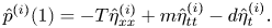 \begin{equation} {\hat p}^{(i)}(1)={-}T\hat\eta_{xx}^{(i)}+m\hat{\eta}_{tt}^{(i)} -d\hat\eta_{t}^{(i)}. \end{equation}
This system has analytical solution in terms of frequency  $\omega$ and wavenumber $k$ given by
 \begin{equation} ({\hat \phi}^{(i)},{\hat p}^{(i)},{\hat \eta}^{(i)}) = \left(\frac{(\omega-U_0 k)}{k} \frac{\sinh(ky)}{\sinh(k)}, \frac{(\omega-U_0 k)^2}{k}\frac{\cosh(ky)}{\sinh(k)},1\right){\hat{\hat \eta}}^{(i)}\cos(k x - \omega t), \end{equation}
where in this case the wave amplitude  ${\hat {\hat \eta }}^{(i)}$ is purely real. Note that this flow profile is irrotational, consistent with the potential flow models of Landahl (Reference Landahl1962) and Benjamin (Reference Benjamin1963). To complete the problem we apply the normal stress balance (A1c) to determine the inviscid dispersion relation
 \begin{equation} D^{(i)}(\omega,k) \equiv \frac{(\omega -U_0 k)^2}{k}\coth(k) + m \omega^2 - T k^2 + i\omega d. \end{equation}
The two normal modes follow from setting  $D^{(i)}(\omega,k) = 0$, and take the explicit form
 \begin{equation} \omega^{(i)}_{{\pm}} = \frac{2k\coth(k)-idk{\pm}(4mTk^2-d^2+4\coth(k)(kT-i U_0 d-mkU_0^2))^{1/2}}{2(\coth(k)+mk)}. \end{equation}
In a similar manner to § 2 we can construct the steady streaming component of the second-order problem and the corresponding Reynolds–Orr energy equation. These are not reproduced here for brevity. However, averaging the energy equation over a wavelength of perturbation it can be written in the form
 \begin{equation} {\hat W}^{(i)}_t ={-}d ({\hat \eta}^{(i)}_t)^2, \end{equation}
where the inviscid activation energy is given by
 \begin{equation} {\hat W}^{(i)}=\frac{1}{4}\left(\frac{(\omega^2 - k^2 U_0^2)}{k} \text{coth}(k) + T k^2 + m \omega^2 \right)({\hat{\hat \eta}}^{(i)})^2 \equiv W^{(i)}({\hat{\hat \eta}}^{(i)})^2. \end{equation}
In this inviscid case we confirm by direct substitution that at neutral stability (Cairns Reference Cairns1979)
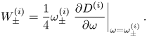 \begin{equation} {W}_{{\pm}}^{(i)} = \frac{1}{4}\omega^{(i)}_{{\pm}} \left.\frac{\partial D^{(i)}}{\partial \omega }\right|_{\omega = \omega_{{\pm}}^{(i)}}. \end{equation}
Interestingly,  $\partial D^{(i)}/\partial \omega$ depends explicitly on the wall damping parameter $d$, but when we substitute the corresponding normal modes (A4) the dependency on $d$ cancels identically. In this case, neutrally stable modes with $W^{(i)}<0$ (termed negative energy waves by Cairns Reference Cairns1979) are class A according to Benjamin's framework, while those with $W^{(i)}>0$ (positive energy waves) are class B and those with $W^{(i)}=0$ are class C.
For a heavy pre-tensioned flexible wall with no wall damping the system is unstable for  $m>T$ (so wall mass is essential for destabilisation), where ${\rm Im} (\omega _+^{(i)})>0$ for $k< k_f$, which satisfies the transcendental equation
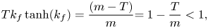 \begin{equation} T k_f \tanh(k_f) = \frac{(m-T)}{m}{=1-\frac{T}{m}<1},\end{equation}
since  $T$,
$T$,  $m>0$. A typical case with $m>T$ is shown in figure 11, plotting the frequency (figure 11a) and activation energy (figure 11b) for both normal modes of the inviscid system. For $k \ge k_f$ we have two neutrally stable modes, one with negative activation energy ( $\omega ^{(i)}_-$, class A) and the other positive ( $\omega ^{(i)}_+$, class B); both modes have positive activation energy for $k>k_d$, which satisfies
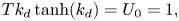 \begin{equation} T k_d \tanh(k_d) = U_0={1},\end{equation}
where  ${\rm Re} (\omega ^{(i)}_-(k_d))=0$. Note that $k_d>k_f$ for all $m$,
$m$,  $T>0$. At $k=k_f$ the two neutrally stable modes of class A and class B coalesce to form a class C flutter mode which is unstable for smaller wavenumbers (Benjamin Reference Benjamin1963; Cairns Reference Cairns1979; Carpenter & Garrad Reference Carpenter and Garrad1986). However, it emerges below that that this mode coalescence is overwhelmed by even mild viscous effects. Conversely, for $m< T$ both normal modes are neutrally stable for all $k$ (the system is never unstable), where again $\omega ^{(i)}_{-}$ transitions from class B to class A as $k$ increases through $k_d$.
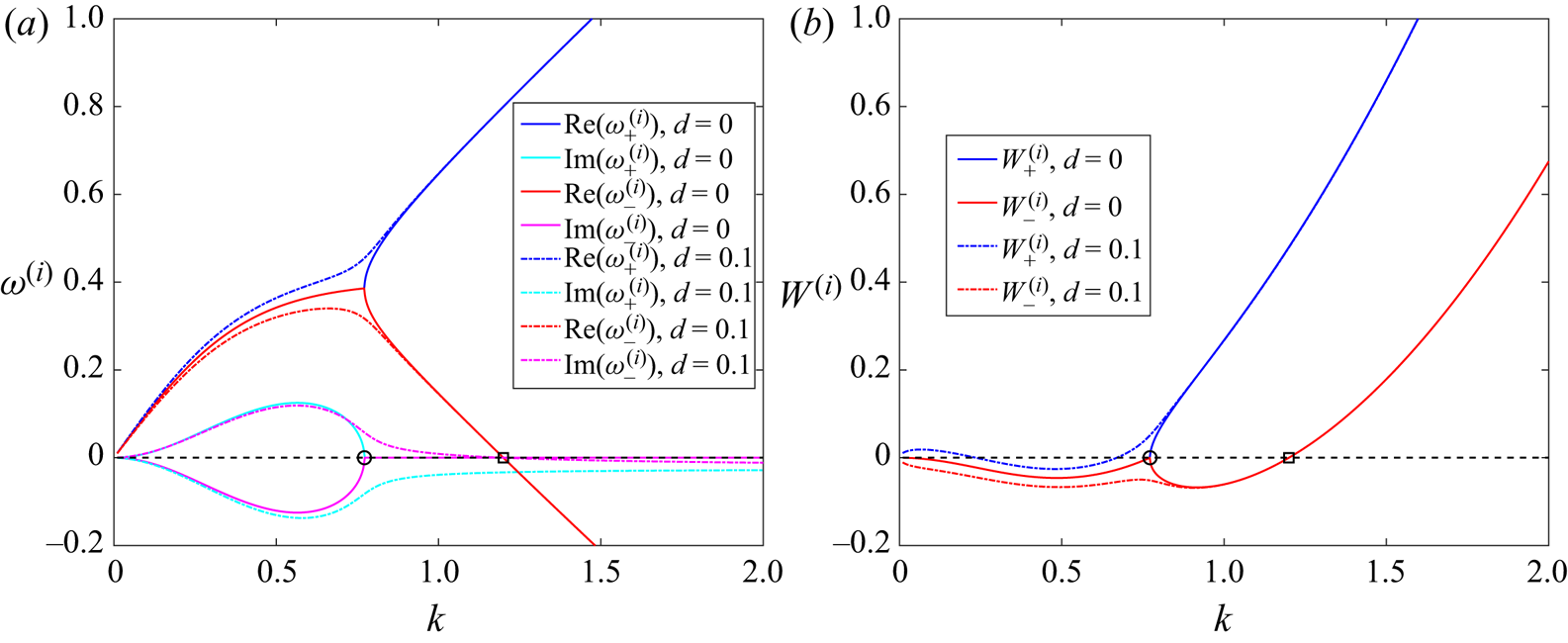
Figure 11. Stability of potential flow through the asymmetric collapsible channel for  $T=1$ and $m=2$ for $d=0$ (solid lines) and $d=0.1$ (dashed lines): (a) the real and imaginary parts of the normal mode frequencies $\omega ^{(i)}_\pm$ as a function of the wavenumber $k$; (b) the activation energy as a function of wavenumber $k$. The open circle is the neutral stability point for zero wall damping (denoted $k_f$, (A6)) while the open square is the neutral stability point for finite wall damping (denoted $k_d$, (A7)).
For potential flow with wall damping we note that neutrally stable modes must have zero frequency ( ${\rm Re} (\omega ^{(i)})=0$) to satisfy the averaged energy budget (A5). Hence, any unstable mode must also have zero activation energy at onset (class C), with corresponding critical wavenumber $k_d$ (A7). To examine how wall damping perturbs the flutter mode, in figure 11 we trace the frequency (figure 11a) and activation energy (figure 11b) when the wall damping is incremented from zero. In this case the two normal modes remain entirely distinct as a function of wavenumber; for $k< k_d$ one normal mode ( $\omega ^{(i)}_-$) is unstable and the other is stable, while for $k>k_d$ both modes are asymptotically stable. This unstable normal mode is destabilised by wall damping.
Hence, in the absence of wall damping, potential flow through a flexible-walled channel is unstable to a class C flutter mode (provided the destabilising influence of wall mass exceeds the stabilising influence of wall tension), which onsets as a coalescence between neutrally stable modes of classes A and B. Conversely, for finite wall damping the coalescence leading to flutter is suppressed and instead one of these normal modes transitions to a class C divergence instability.


 Open access