


1. Introduction
The phenomena of liquid bridge stretching were first studied by Plateau (Reference Plateau1864), Stefan (Reference Stefan1875) and Rayleigh (Reference Rayleigh1878) more than a hundred years ago. Since then, the dynamics of liquid jets and bridges have been studied extensively. Several comprehensive reviews of this field present state-of-the-art modelling approaches (Schulkes Reference Schulkes1993; Yarin Reference Yarin1993; Eggers Reference Eggers1997; Villermaux Reference Villermaux2007; Eggers & Villermaux Reference Eggers and Villermaux2008).
Liquid jet or liquid bridge stretching is a phenomenon relevant to many practical applications like rheological measurements, atomisation, crystallisation, car soiling, oil recovery and typical industrial printing processes, such as gravure, flexography, lithography and roll coating (Ambravaneswaran & Basaran Reference Ambravaneswaran and Basaran1999; Marmottant & Villermaux Reference Marmottant and Villermaux2004; Gordillo & Gekle Reference Gordillo and Gekle2010; Jarrahbashi et al. Reference Jarrahbashi, Sirignano, Popov and Hussain2016; Gaylard, Kirwan & Lockerby Reference Gaylard, Kirwan and Lockerby2017; Xu et al. Reference Xu, Zhang, Fu and Huang2017). The dynamics of liquid bridges also govern coalescence processes of solid wetted particles (Crüger et al. Reference Crüger, Salikov, Heinrich, Antonyuk, Sutkar, Deen and Kuipers2016).
A broad class of models have been developed for relatively long jets. The long-wave approach for a nearly cylindrical jet describes well, for example, the transverse instability of a jet exposed to airflow, introduced by Entov & Yarin (Reference Entov and Yarin1984). A slender jet model was also used by Eggers & Dupont (Reference Eggers and Dupont1994) and Eggers (Reference Eggers1993) to show that liquid bridge pinching is universal but asymmetric in the pinching region for pinned liquid bridges. Papageorgiou (Reference Papageorgiou1995) later introduced an alternative model with a symmetric geometry solution in the pinching region. A more recent study of Qian & Breuer (Reference Qian and Breuer2011) has shown the effects of surface wettability and moving contact lines on liquid bridge break-up behaviour for stretching speeds up to 600  ${\rm \mu }$m s $^{-1}$. Further studies use this long-wave approach to show the importance of the pinching position for the break-up time (Yildirim & Basaran Reference Yildirim and Basaran2001) or the behaviour of non-Newtonian liquids on bridge thinning and break-up behaviour (Anna & McKinley Reference Anna and McKinley2000; McKinley Reference McKinley, Binding and Walters2005).
If the height of a liquid bridge ( $H_0$) is much smaller than its diameter ( $D_0$), the dimensionless height is $\lambda \ll 1$ with $\lambda =H_0/D_0$, and therefore the modelling approach has to be different from that of previous studies. For such cases, the surface of the liquid bridge can become unstable because of the high interface retraction rates and small initial liquid bridge heights. Due to the small initial heights and large initial diameter, the conditions are similar to those in Hele-Shaw flow cells.
Frequently observed phenomena are finger patterns formed from growing instabilities in fixed-height Hele-Shaw cells for transverse (Saffman & Taylor Reference Saffman and Taylor1958) or radial (McCloud& Maher Reference McCloud and Maher1995; Mora & Manna Reference Mora and Manna2009) flows. The study by Maxworthy (Reference Maxworthy1989) compares modified wavenumber theories based on the fastest growing mode from Park, Gorell & Homsy (Reference Park, Gorell and Homsy1984) and Schwartz (Reference Schwartz1986) to experiments in radial flows. Paterson (Reference Paterson1981) derived a prediction for the number of fingers formed at a radially expanding interface of the liquid spreading between two fixed substrates.
The problem is entirely different if the flow is caused by the motion of substrates and the gap thickness changes in time. For example, the rate equation for the displacement of a liquid bridge under a defined pulling force is investigated in the study by Ward (Reference Ward2011). The measurements from Amar & Bonn (Reference Amar and Bonn2005) were conducted at very low stretching speeds of 20–50  ${\rm \mu }$m s $^{-1}$, high viscosities of 30 Pa s and large initial heights. For a lifting Hele-Shaw cell, Nase, Derks & Lindner (Reference Nase, Derks and Lindner2011) developed a model for the interfacial stability of the liquid bridge, leading to a prediction of the maximum number of fingers. Dias & Miranda (Reference Dias and Miranda2013a), Shelley, Tian & Wlodarski (Reference Shelley, Tian and Wlodarski1997), Sinha et al. (Reference Sinha, Kabiraj, Dutta and Tarafdar2003), Amar & Bonn (Reference Amar and Bonn2005) and Spiegelberg & McKinley (Reference Spiegelberg and McKinley1996) studied liquid bridge stretching in lifted Hele-Shaw set-ups. In most of these cases, the stretching speed is constant and is relatively small, such that inertial effects are comparably small.
The analysis of fingering instability has been further generalised by Dias & Miranda (Reference Dias and Miranda2013a), where the influence of radial viscous stresses at the meniscus has been taken into account. For identifying the most unstable mode, the maximum amplitude has to be considered instead of the usual approach of selecting the fastest growing modes. This approach accounts for the non-stationary effects in the flow, even if the substrate velocity is constant. The amplitude growth due to the disturbances is not exponential since the parameters of the problem, mainly the thickness of the gap, change in time. More recently, Anjos, Dias & Miranda (Reference Anjos, Dias and Miranda2017) showed in an analytical and numerical study that inertia has a significant impact on finger formation at higher velocities, especially on dendritic-like structures on the fingertips.
In this study, the flow in a thin liquid bridge between two substrates, generated by an accelerating downward motion of the lower substrate, is studied experimentally and modelled theoretically. This situation is a generic model for processes like gravure printing or water splash due to a tyre rolling on a wet road. The novel feature of this study is that the substrate can be moved with very high accelerations. In the conducted parameter studies, accelerations up to 180 m s $^{-2}$ are investigated. The stretching of the liquid bridge between the two substrates is observed using a high-speed video system. In the experimental part, finger formation of the fluid bridge is characterised, and the number of fingers is measured.
Linear stability analysis of the liquid bridge accounts for the inertial term, the viscous stresses and capillary forces in the fluid flow, and allows the prediction of the maximum number of fingers. This number is obtained using the mode exhibiting the highest amplification rate to interface perturbations. The second criterion for the fingering threshold is associated with the limiting value of the dimensionless wave amplitude. Both requirements lead to the same scaling of the threshold parameter for fingering and agree well with the experimental observations.
It should be noted that in this study the number of fingers is predicted as a function of the substrate acceleration in a lifted Hele-Shaw cell, whereas most previous studies were based on experiments in fixed or lifting Hele-Shaw cells with significantly lower lifting velocities. Those predictions (e.g. Saffman & Taylor Reference Saffman and Taylor1958; Park et al. Reference Park, Gorell and Homsy1984; Schwartz Reference Schwartz1986; Maxworthy Reference Maxworthy1989) deviate significantly from the present measurement results due to physical differences among the experiments. In other words, since no characteristic velocity exists (only acceleration  $a$), the main dimensionless numbers, like the capillary number $\mathit {Ca}$, are defined completely differently. It is important to note that the physical mechanism of instability in all these problems is the same. The pressure gradient causes instability in the liquid at the interface. This mechanism is thus analogous to the Rayleigh–Taylor instability.
2. Experimental method
2.1. Experimental set-up and procedure
The experimental set-up for stretching a liquid bridge is shown schematically in figure 1(a). The stretching system consists of two substrates orientated horizontally. The lower substrate is mounted on a linear drive which allows accelerations from 10 to 180 m s $^{-2}$. The positional accuracy of the linear drive is about 5 $ {\rm \mu }$m. The upper substrate is fixed. Both substrates are transparent, fabricated from glass with a roughness of $R_a = 80\,{\rm nm}$. The initial thickness of the gap in the experiments, $H_0$, varies from 20 to 140 $ {\rm \mu }$m, as shown later in figure 5. The static contact angle between the $Gly50$/ $Gly80$ liquid and the glass substrates is $\theta \approx 40^{\circ }$. The measurements for hydrophobic substrates are performed on silanised glass wafers (Hartmann & Hardt Reference Hartmann and Hardt2019) with a static contact angle between substrate and $Gly50$/ $Gly80$ of $\theta \approx 110^{\circ }$.
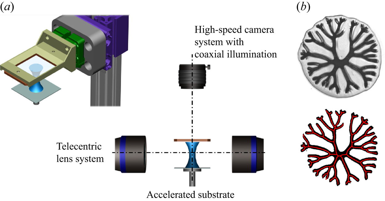
Figure 1. Experimental method: (a) the set-up and (b) post-processing of images.
A microlitre syringe is used as a fluid dispensing system. To investigate the effect of the liquid properties, two water–glycerol mixtures with different viscosities are used:  $Gly50$ with viscosity $\mu =5.52\times 10^{-3}$ Pa s, surface tension $\sigma =67.3\times 10^{-3}$ N m $^{-1}$ and density $\rho =1129$ kg m $^{-3}$; and $Gly80$ whose properties are $\mu =5.36\times 10^{-2}$ Pa s, $\sigma =65.5\times 10^{-3}$ N m $^{-1}$ and $\rho =1211$ kg m $^{-3}$. The possible variation of the liquid properties with temperature is accounted for in the data analysis.
To investigate the influence of the geometry parameter on the bridge strain, the liquid volumes of the bridge are varied in this study between  $1$ and 5 $ {\rm \mu }$l. This allows variation of the initial height-to-diameter ratio, $\lambda = H_0/D_0$, in the range $0.003<\lambda <0.2$.
The observation system consists of two high-speed video systems. The side-view camera is equipped with a telecentric lens. The camera on top uses a  $12\times$ zoom lens system. The images are captured with a resolution of one megapixel at a frequency of 12.5 kfps.
The post-processing for the top view was performed using trainable weka (Arganda-Carreras et al. Reference Arganda-Carreras, Kaynig, Rueden, Schindelin, Eliceiri, Cardona and Seung2017), a machine learning algorithm, assisting with the segmentation of the images. Afterwards, the images were skeletonised and the number of fingers was counted. An example of the segmentation and skeleton is shown in figure 1(b) and later in figure 7 the number of fingers is plotted against  $R/R_0$.
2.2. Observations of bridge stretching
The experimental set-up allows shadowgraphy images of the contact area between substrate and liquid to be captured during the stretching process. An example of a side-view, high-speed visualisation of a stretching  $Gly80$ bridge is shown in figure 2(a). In this example, the substrate acceleration is 180 m s $^{-2}$ and the initial height is 20 $ {\rm \mu }$m. The initial liquid bridge height-to-diameter ratio is $\lambda =0.02$. During the stretching process, the diameter in the middle of the bridge, $D_M$, reduces and a thin liquid film remains on both substrates. The contact line remains pinned for all experiments performed, evident from the top views in figure 3. After 12.6 ms the bridge pinches off. In figure 2(b) the evolution of the scaled bridge diameter during stretching is shown as a function of the dimensionless gap width. For the stage when $H \ll D_M$, the evolution of the bridge diameter is universal and it does not depend on the substrate acceleration or liquid properties.
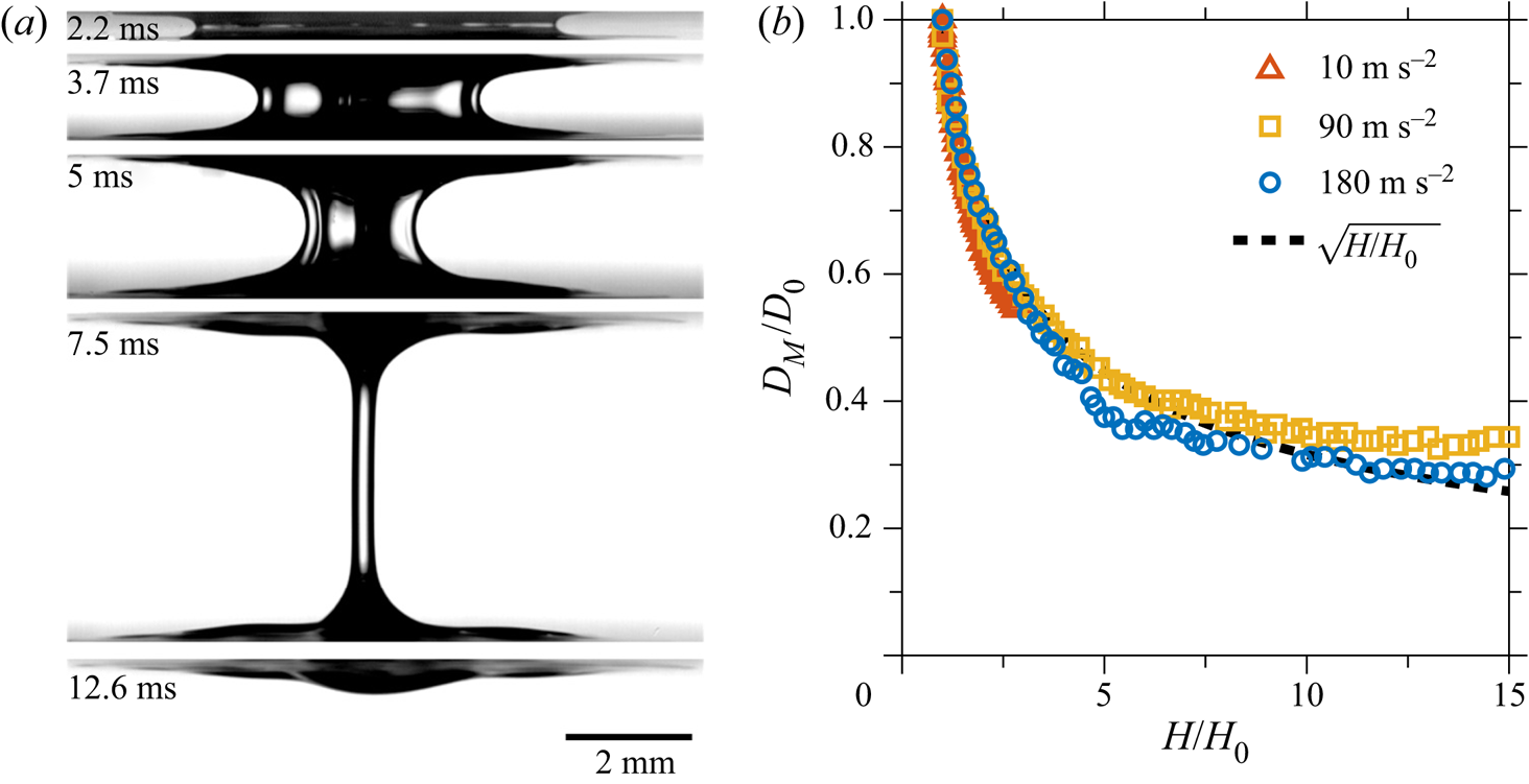
Figure 2. Evolution of the diameter of a liquid bridge. (a) Side views of a  $Gly80$ bridge stretched with a constant acceleration of 180 m s $^{-2}$. The initial gap is 20 $ {\rm \mu }$m and the gap-to-diameter ratio is $\lambda = 0.02$. (b) The scaled bridge middle diameter $D_M/D_0$ as a function of the dimensionless gap width $H/H_0$ for various substrate accelerations. The curve corresponds to the predictions based on (3.2).
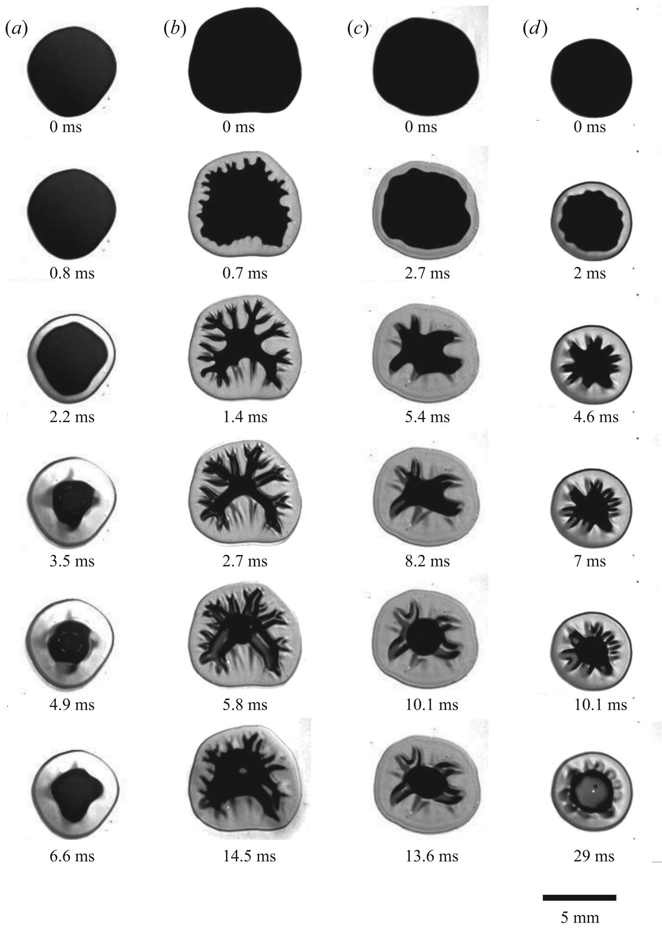
Figure 3. Top view of the receding interface due to bridge stretching under various experimental conditions: (a) liquid  $Gly50$, substrate acceleration $a=180$ m s $^{-2}$, relative gap width $\lambda =0.03$; (b) $Gly50$, $a=180$ m s $^{-2}$, $\lambda =0.006$; (c) $Gly50$, $a=10$ m s $^{-2}$, $\lambda =0.06$; (d) $Gly80$, $a=10$ m s $^{-2}$, $\lambda =0.03$. Contact angles are $\theta \approx 40^{\circ }$ for $Gly50$ and $Gly80$ on the glass substrate.
Several typical top views of the liquid bridge through the transparent substrate are shown in figure 3 at different instants for various experimental parameters. In some cases, the onset of instability can be clearly seen, which leads to the appearance of a net of fingers. The most stable case in figure 3(a) is obtained with a relatively wide gap and low acceleration. The most unstable case, associated with the highest number of fingers, corresponds to the highest accelerations and smaller initial gap widths, as shown in the example in figure 3(b). In the example in figure 3(c), fingers can be observed even with relatively small substrate acceleration, but only for small dimensionless heights  $\lambda$. Figure 3(d) shows how increased liquid viscosity leads to an evolved finger pattern. Increasing the substrate acceleration or viscosity enhances the fingering instability, whereas, with an increasing dimensionless height $\lambda$, finger formation is mitigated.
The main part of this study was conducted using glass substrates with a static contact angle of  $\theta \approx 40^{\circ }$, as shown in figure 3. As already mentioned, the outer contour of the bridge remains almost stationary during finger formation. To investigate the effect of wettability on the fingering instability, also measurements with different contact angles were performed. The reference measurements were executed on hydrophobic silanised glass substrates with static contact angles of $\theta \approx 110^{\circ }$, as shown in figure 4. Since a higher contact angle results in a higher contact line speed (Hoffman Reference Hoffman1975; Voinov Reference Voinov1976; Dussan Reference Dussan1979; Tanner Reference Tanner1979), an effect on the fingering instability is more likely. In direct comparison to figure 3, it is evident that the contact line movement starts earlier, and therefore the contact line speed is higher. It is also observable from figure 4 that the contact line also stays immobile during finger formation and starts to move after the fingers have already begun to disintegrate, at times of around 9.04 ms. Therefore the dewetting does not seem to affect the fingering instability due to their subsequent appearance.
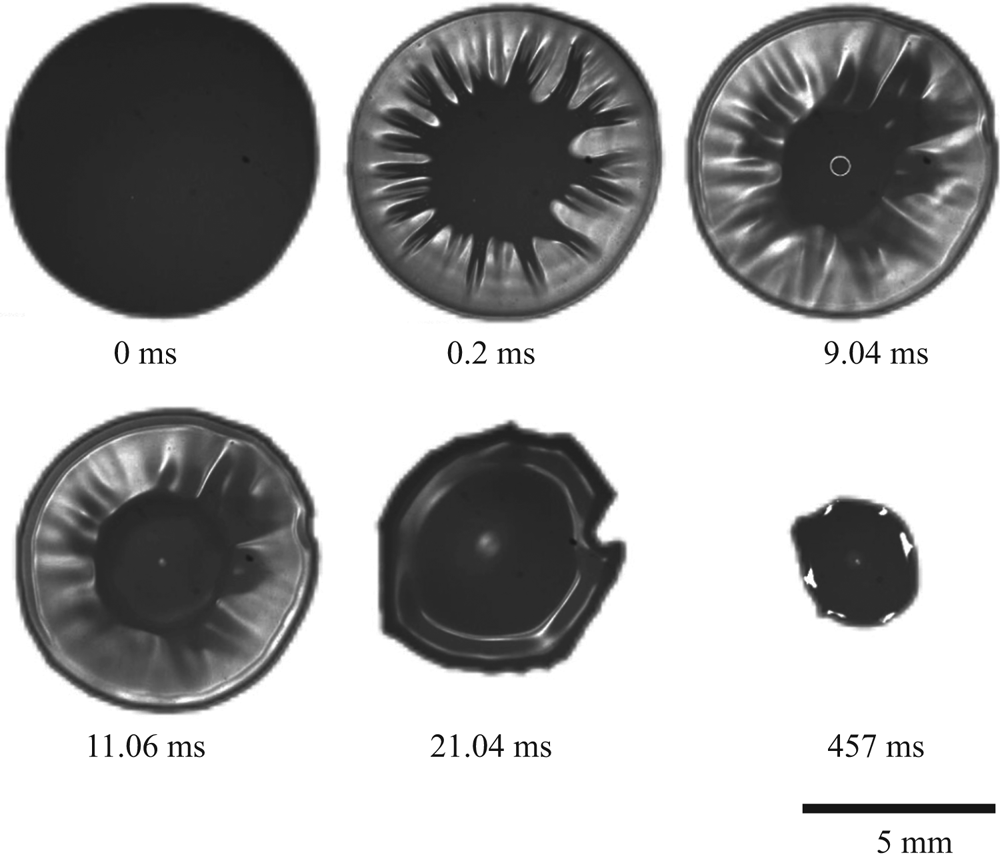
Figure 4. Sequence of bottom views of the liquid bridge and the wetted spot at different instants. The time associated with the fingering (approximately  $10^{-1}$ ms) is one order of magnitude smaller than the time at which the dewetting process becomes notable, at approximately 20 ms. Contact angles for the hydrophobic substrates are $\theta \approx 110^{\circ }$ for $Gly50$ and $Gly80$.
3. Stability analysis of the bridge interface
In this study, a stability analysis is performed based on experimental measurements of the flow in a thin gap between two substrates. The problem is linearised in the framework of the long-wave approximation.
3.1. Basic flow
The flow field in a stretching liquid bridge can be subdivided into two main regions: the meniscus region and the central, inner region, which is not influenced by the meniscus. The solution for an axisymmetric creeping flow between two parallel substrates, one of which moves, is well known (Landau & Lifshitz Reference Landau, Lifshitz, Sykes and Reid1959). The axial and the radial components of the velocity field are
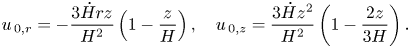 \begin{equation} u_{\,{0,r}} = -\frac{3 \skew4\dot{H} r z}{H^{2}} \left(1-\frac{z}{H}\right), \quad u_{\,{0,z}} = \frac{3\skew4\dot{H} z^{2}}{H^{2}} \left(1-\frac{2 z}{3 H}\right). \end{equation}
This velocity field satisfies the equation of continuity, the momentum balance equation and the kinematic conditions at both substrates. Unfortunately, this solution does not apply to the case when the effect of the substrate acceleration becomes significantly high. Moreover, the expression for the velocity field between two substrates (3.1) is not applicable at the interface of the meniscus. It does not satisfy the conditions for the pressure at the interface, determined by the Young–Laplace equation, and it does not satisfy the conditions of zero shear stress at this interface. Moreover, this velocity field is not able to accurately predict the rate of change of the meniscus radius  $\skew4\dot{R}$. Assuming the rate of change of the minimum meniscus radius at the middle plane as $\skew4\dot{R} = u_{\,0,r}$ at $z= H/2$, and using (3.1), the solution of the equation for the meniscus propagation becomes $R=R_0 (H_0/H)^{3/16}$. This solution does not agree with the experimental data for the evolution of the meniscus radius. Therefore, the flow in the meniscus region has to be treated differently.
An expression for the radius and the height can be derived from the overall mass balance, where the initial thickness is  $H_0$, the initial radius is $R_0$ and the lower substrate moves with a constant acceleration $a$. The radius of the bridge meniscus, $R(t)$, can be estimated as
 \begin{equation} R(t)=R_0 \left[\frac{H_0}{H(t)}\right]^{1/2}, \quad H(t) = H_0 + \frac{a t^{2}}{2}, \end{equation}
which gives a valid estimate for the initial times, when  $R(t)\gg H(t)$, as demonstrated in figure 2(b).
The flow in the meniscus region has to be treated separately. This flow has to satisfy the boundary conditions at the curved meniscus interface and must also include the corner flows (Moffatt Reference Moffatt1964; Anderson & Davis Reference Anderson and Davis1993). The model of the meniscus flow is not trivial and can lead to multiple solutions (Gaskell et al. Reference Gaskell, Savage, Summers and Thompson1995). However, an accurate solution for the meniscus stability problem has to be based on the meniscus velocity field, since the stresses in this region govern the meniscus instability.
In this study, it is assumed that the main reason for the meniscus instability is the appearance of a normal pressure gradient at the meniscus interface. This mechanism is analogous to the Rayleigh–Taylor instability, where the pressure gradient is caused by gravity or by the interface acceleration. This approximate solution is valid only for the case of a very small relative gap thickness,  $\lambda \ll 1$. Note also that the ratio of the axial and radial components of the liquid velocity is comparable with $\lambda$. The stresses associated with the axial flow are therefore much smaller than those associated with the radial velocity component.
In the following, only the dominant terms of the pressure gradient at the interface are considered. The pressure gradient includes the viscous stresses and the inertial terms associated with the material acceleration of the meniscus  $\ddot R$. The approximation is based on the fact that the radial velocity in the liquid at the interface at the middle plane $(z=H/2)$ is equal to $\skew4\dot{R}$. The value of the pressure gradient is then estimated from the Navier–Stokes equations with the help of (3.2) in the form
 \begin{equation} p_{\, 0,r}= - b \mu \frac{\skew4\dot{R}}{H(t)^{2}} - \rho \ddot R = \mu a t b\frac{ \sqrt{H_0} R_0}{2 H^{7/2}}+\rho a \frac{ \sqrt{H_0} R_0 }{2 H^{5/2}}(H_0-a t^{2}), \end{equation}
where  $b$ is a dimensionless constant. Its value $b\approx 12$ can be roughly estimated approximating the velocity profile by a parabola, as in the gap-averaged Darcy's law (Bohr, Brunak & Nørretranders Reference Bohr, Brunak and Nørretranders1994; Shelley et al. Reference Shelley, Tian and Wlodarski1997; Amar & Bonn Reference Amar and Bonn2005; Dias & Miranda Reference Dias and Miranda2013b).
Approximation (3.3) is valid only for the cases of  $\lambda \ll 1$ considered in this study. Since the ratio of the axial to the radial velocity, which can be estimated from (3.2), is comparable with $\lambda$, the effect of the axial velocity on the pressure gradient is negligibly small.
3.2. Planar interface, long-wave approximation of small flow perturbations
Since the radius of the liquid bridge is much larger than the gap thickness,  $R \gg H$, the flow leading to small interface disturbances can be considered in a Cartesian coordinate system $\{x, y\}$, where the $x$ coordinate coincides with the radial direction normal to the meniscus, defined as $x=0$, and the $y$ direction is tangential to the meniscus. The kinematic relation (3.2) allows the evaluation of the necessary condition $R \gg H$, which is satisfied at times $t\ll \sqrt {2 (R_0-H_0)/a}$. In all our experiments this condition is satisfied.
The coordinate system  $\{x, y\}$ is fixed at the meniscus of the liquid bridge, such that
 \begin{equation} r = R(t) + x. \end{equation}
 The small flow perturbations, in the direction normal to the substrates, are neglected. Liquid flow occupies the semi-infinite space  $x\in\;]-\infty ;\;0]$. Denote $\{u'(x,y,t); \;v'(x,y,t)\}$ as the velocity vector of the flow perturbations, averaged through the gap width, and $p'(x,y,t)$ is the pressure perturbation. The absolute velocity and the pressure $p$ in the gap can be expressed in the form
 \begin{equation} u = \skew4\dot{R}(t) + u'(x,y,t),\quad v = v'(x,y,t),\quad p = p_0(x,t) + p'(x,y,t). \end{equation}
Therefore, the time derivatives of the components of the velocity field can be written in the form
 \begin{equation} u_{\, ,t}= \ddot R + u'_{\, ,t} - \skew4\dot{R} u'_{,x}, \quad v_{,t}= v'_{,t} - \skew4\dot{R} v'_{,x}. \end{equation}
 The gap thickness  $H$ is assumed to be the smallest length scale in the problem. In this case, consideration of only the dominant terms in the Navier–Stokes equation, written in the accelerating coordinate system, yields
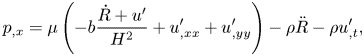 \begin{gather} p_{,x} = \mu \left(-b \frac{\skew4\dot{R}+ u'}{H^{2}} + u'_{,xx} + u'_{,yy}\right) - \rho \ddot R - \rho u'_{,t}, \end{gather}
 \begin{gather}p_{,y} = \mu \left(-b \frac{v'}{H^{2}} + v'_{,xx} + v'_{,yy}\right) - \rho v'_{,t}. \end{gather}
 The characteristic value of the leading viscous terms in the pressure gradient expressions (3.7a) and (3.7b) is  $\mu b u'/H_0^{2}$. The characteristic time of the problem is $\sqrt {H_0/a}$. Therefore, the inertial terms of the flow fluctuations are of order $\rho u'_{,t}\sim \rho u' \sqrt {a/H_0}$. The Reynolds number, defined as the ratio of the inertial and viscous terms, is therefore
 \begin{equation} \mathit{Re} = \frac{a^{1/2} H_0^{3/2}\rho}{b \mu}. \end{equation}
In all experiments, the Reynolds number is of the order of  $10^{-2}$. The inertial effects associated with the flow fluctuations are therefore negligibly small. The governing equation for the velocity perturbation can then be obtained from (3.7a) and (3.7b), neglecting the terms $\rho u'_{,t}$ and $\rho v'_{,t}$:
 \begin{equation} -b \frac{u'_{,y}-v'_{,x}}{H^{2}} + u'_{,xxy} + u'_{,yyy} - v'_{,xxx} - v'_{,yyx}=0. \end{equation}
 The velocity field  $\{u', v'\}$ has to satisfy (3.9) as well as the continuity equation and the condition of the shear-free meniscus surface:
 \begin{gather} u'_{,x}+v'_{,y}=0 , \end{gather}
 \begin{gather} u'_{,y}+v'_{,x}=0, \quad \mathrm{at}\ x=0. \end{gather}
 Consider the sinusoidal profile of the flow fluctuations along the  $y$ direction. This means that both velocity components include the term $\exp (\textrm {i} k y)$, where $k$ is the wavenumber. The corresponding velocity field for the velocity of the small flow disturbances satisfying (3.9)–(3.10b) is
 \begin{gather} u' = \left( \exp(kx)-\frac{2H^{2}k^{2}}{b+2H^{2}k^{2}}\exp\left[\frac{\sqrt{b+H^{2} k^{2}}}{H}x\right]\right)\exp(\textrm{i} k y ) T(t), \end{gather}
 \begin{gather}v' =\textrm{i}\left( \exp(kx)-\frac{2H k \sqrt{b+H^{2} k^{2}}}{b+2H^{2}k^{2}}\exp\left[\frac{\sqrt{b+H^{2} k^{2}}}{H}x\right]\right)\exp(\textrm{i} k y ) T(t), \end{gather}
where  $T(t)$ is a function of time.
The small perturbations of the meniscus shape, defined as  $x=\delta (y,t)$, are determined by the normal velocity component $u$ at the meniscus $x=0$. The boundary conditions for the meniscus perturbations, $\delta _{,t}=u$ at $x=0$, yield
 \begin{equation} \delta = \exp(\textrm{i} k y) G(t),\quad \mathrm{with} \quad T(t) =\frac{b+2 H^{2} k^{2}}{b} \dot G(t). \end{equation}
 The pressure increment, associated with the flow perturbations at the interface,  $p'$, is determined by the capillary forces and viscous stress:
 \begin{equation} p'(x,t) =- \sigma \delta_{,yy}-2 \mu u_{,x},\quad \mathrm{at}\ x =\delta(y,t). \end{equation}
 The total pressure near the meniscus also depends on the curvature in the plane normal to the substrate. In this study, the dependence of the shape of the meniscus in this plane on  $\delta (y,t)$ is neglected, since the capillary pressure associated with this curvature is approximated by $p\sim \sigma /H$. Thus, this pressure does not depend on the $y$ coordinate and does not contribute to flow stability.
The pressure  $p'$ at position $x=0$ can be approximated accounting for the smallness of the shape deformation:
 \begin{equation} p' =- \sigma \delta_{,yy} - \delta p_{0,r}-2 \mu u_{,x},\quad \mathrm{at}\ x =0, \end{equation}
where  $p_{0}$ is the pressure gradient at the meniscus of the basic flow, determined in (3.3). The term $\delta p_{0,r}$ appears as a result of linearisation of the pressure terms in the neighbourhood of the liquid bridge interface.
Substituting (3.14) in expression (3.7b) yields, with the help of (3.11a)–(3.12), the following ordinary differential equation for the function  $G(t)$:
 \begin{equation} b (k^{3} \sigma -k p_{0,r}) H^{2} G(t) + \big[4 H^{3} k^{3}\big(\sqrt{H^{2} k^{2}+b}-H k \big) +b^{2}\big] \mu \dot G(t)=0. \end{equation}
The solution of the ordinary differential equation (3.15) is
 \begin{equation} G(t) = \delta_0 \exp\left[-\frac{b}{\mu}\int_0^{t} \frac{ H^{2} \big(k^{3} \sigma -k p_{0,r}\big)}{4 H^{3} k^{3}\big(\sqrt{H^{2} k^{2}+b}-H k\big) +b^{2} }\,\mathrm{d}t\right], \end{equation}
where  $\delta _0$ is the initial meniscus perturbation.
The function  $G(t)$ in (3.16) can be derived using (3.2) and (3.3). It can be expressed in dimensionless form as
 \begin{gather} G=\delta_0\exp\left[ \frac{\sqrt{b}}{2\lambda}\int_0^{\tau}\Omega(\xi,\tau)\,\mathrm{d}\tau\right], \end{gather}
 \begin{gather}\Omega=\frac{\tau \xi (\tau ^{2}+1)^{-3/2} -\dfrac{\xi ^{3}}{\mathit{Ca}}{(\tau ^{2}+1)^{2}} + \dfrac{\mathit{Re}(1-2 \tau^{2}) \xi }{\sqrt{2} \sqrt{\tau^{2}+1}} }{1-4 (\tau ^{2}+1)^{3} \xi ^{3} [\xi (\tau ^{2}+1) -\sqrt{(\tau ^{2}+1)^{2} \xi ^{2}+1}]}, \end{gather}
where the dimensionless time  $\tau$, the dimensionless wavenumber $\xi$ and the capillary number $\mathit {Ca}$ are defined as
 \begin{equation} \tau = t\sqrt{\frac{a}{2 H_0}}, \quad \xi = \frac{k H_0}{\sqrt{b}},\quad \mathit{Ca}=\frac{\sqrt{a} \mu R_0}{\sqrt{2 H_0} \sigma }. \end{equation}
The Reynolds number is defined in (3.8) and the geometrical parameter is  $\lambda = H_0/2 R_0$, as defined in § 2.
Equations (3.17) and (3.18) allow computation of the evolution of the amplitude of waves for a given wavelength and given parameters of liquid bridge stretching.
In figure 6 the dimensionless amplitude of the perturbations of the bridge radius  $\ln (G/\delta _0)$, computed using (3.17), is shown as a function of the dimensionless wavenumber $\xi$ for various times $\tau$. In the cases shown in figure 6(a,b), corresponding to a large number of fingers, the absolute amplitude of the perturbation $G$ is two orders of magnitude higher than the amplitude of the initial perturbations $\delta _0$. In the case of figure 6(c) close to the fingering threshold, $G/\delta _0\sim 10^{1}$, while in the case shown in figure 6(d), in which no apparent fingering has been observed, the value of $G/\delta _0$ is of order unity. In each of the cases shown in figure 6(a) the wavenumber corresponding to the maximum amplitude is only slightly dependent on time, but is significantly influenced by the parameters of bridge stretching.
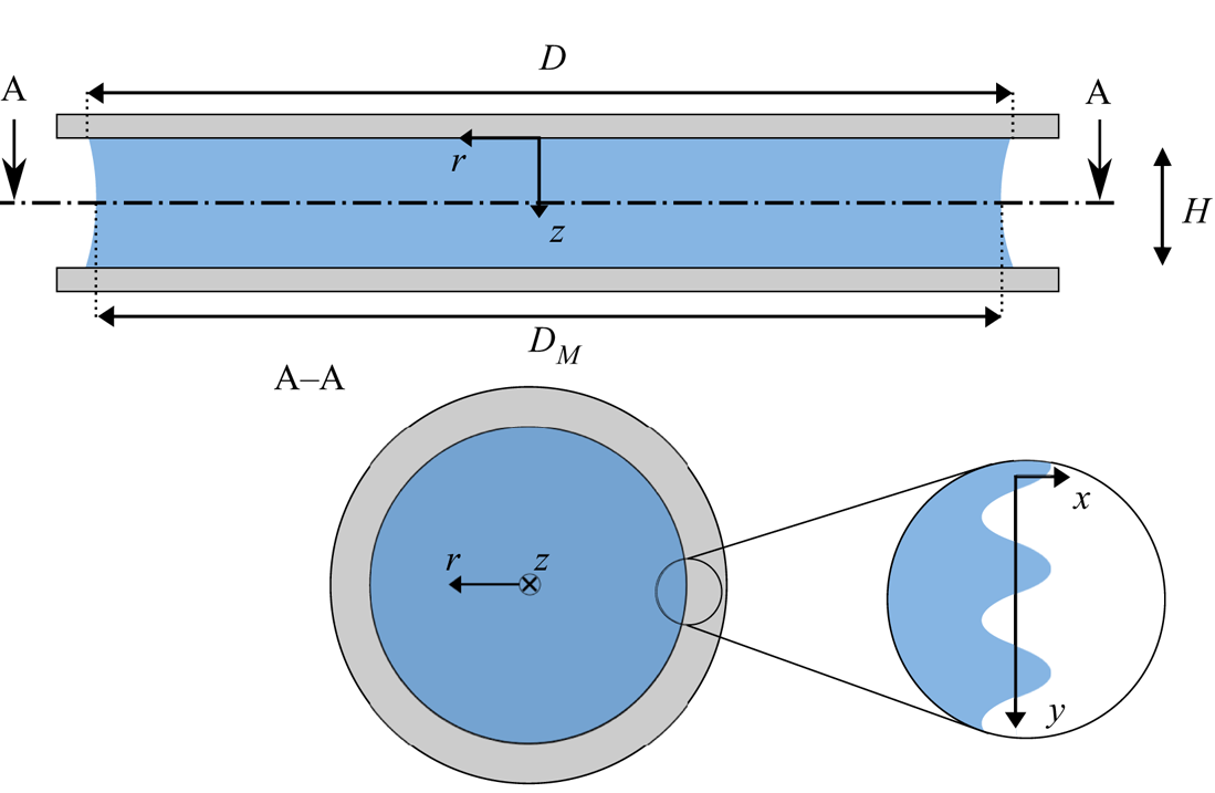
Figure 5. A cylindrical frame of reference is used at the symmetry axis ( $r, z$). The area of interest for instability analysis is magnified, and a Cartesian frame of reference is used at the interface $\{x, y\}$.
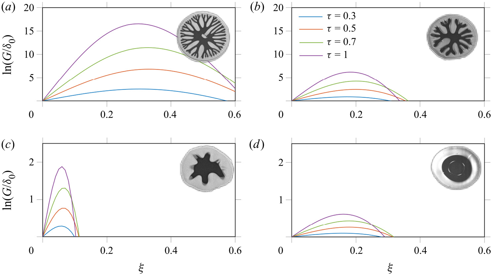
Figure 6. Dimensionless amplitude of radius perturbations  $\ln (G/\delta _0)$ as a function of the dimensionless wavenumbers $\xi$ for various time instants $\tau$, computed by numerical integration of (3.16): (a) $\mathit {Ca}=2.45$, $\mathit {Re}=0.005$, $\lambda =0.0059$; (b) $\mathit {Ca}=0.704$, $\mathit {Re}=0.0026$, $\lambda =0.0099$; (c) $\mathit {Ca}=0.0663$, $\mathit {Re}=0.0252$, $\lambda =0.0109$; and (d) $\mathit {Ca}=0.5109$, $\mathit {Re}=0.034$, $\lambda =0.0902$.
3.3. Approximation for small capillary numbers
In the long-wave approximation, values of  $\xi$ are assumed to be small. This assumption can again be examined after the solution for typical values of $\xi$ has been obtained. In this study, only the dominant terms are taken into account, while the terms of $O(\xi ^{4})$ are neglected. The corresponding approximate expression for $\int _0^{\tau }\Omega \,\mathrm {d}\tau$ is derived in the form
 \begin{align} \int_0^{\tau}\Omega(\xi,\tau)\,\mathrm{d}\tau &=\xi-\frac{\tau (3 \tau ^{4}+10 \tau ^{2}+15) \xi ^{3}}{15 \mathit{Ca}}-\frac{\xi }{\sqrt{\tau ^{2}+1}}\nonumber\\ &\quad -\frac{\mathit{Re} \xi}{\sqrt{2}}\big(\tau \sqrt{\tau ^{2}+1}-2\,\mathrm{arcsinh}\,\tau \big)+O(\xi^{4}). \end{align}
 The most unstable mode  $\xi _\ast$ associated with the maximum positive value of the function $\int _0^{\tau }\Omega \,\mathrm {d}\tau$ is therefore
 \begin{equation} \xi_\ast =\sqrt{\mathit{Ca}}\left[\frac{1-\dfrac{1}{\sqrt{\tau ^{2}+1}}+ \dfrac{\mathit{Re}}{\sqrt{2}}(\tau \sqrt{\tau ^{2}+1}-2\,\mathrm{arcsinh}\,\tau )}{\tau \left(\dfrac{3}{5} \tau ^{4}+2 \tau ^{2}+3\right)}\right]^{1/2}. \end{equation}
 The dimensionless time  $\tau$ is of the order of unity. The value of the dimensionless wavenumber also has to be small in the framework of the long-wave approximation used in this study. Therefore, the solution (3.21) for the most unstable mode $\xi _*$ is valid only for small capillary numbers.
The wavelength of the most unstable mode is  $\ell _\ast =2{\rm \pi} /k$. The number of finger-like jets is therefore
 \begin{equation} N_f=2{\rm \pi} {R}/\ell_\ast= \frac{\sqrt{b}}{2\lambda} \frac{\xi_\ast}{\sqrt{1+\tau^{2}}}. \end{equation}
The expression for the number of fingers is obtained using (3.21):
 \begin{equation} N_f = \frac{\sqrt{b \mathit{Ca}}}{2\lambda}\left[\frac{1-\dfrac{1}{\sqrt{\tau ^{2}+1}}+ \dfrac{\mathit{Re}}{\sqrt{2}}(\tau \sqrt{\tau ^{2}+1}-2\,\mathrm{arcsinh}\,\tau )}{\tau (\tau ^{2}+1) \left(\dfrac{3}{5} \tau ^{4}+2 \tau ^{2}+3\right)}\right]^{1/2}. \end{equation}
 The predicted number of fingers depends on the dimensionless time  $\tau$. Such dependence is confirmed by observations.
4. Results and discussion
The maximum value of the function  $N_f(\tau )$ can be computed from (3.23). In the limit $\mathit {Re}=0$, the maximum,
 \begin{equation} N_{{\textit{max}}}\approx 0.38 \sqrt{\mathit{Ca}}/\lambda,\quad \mathit{Ca} \ll 1,\quad \mathit{Re} =0, \end{equation}
is reached at the instant  $\tau _\star \approx 0.49$. The predicted bridge radius $R$ corresponding to the maximum number of jets is therefore $R_\star =R_0(1+\tau _\star ^{2})^{-1/2}\approx 0.9 R_0$.
In figure 7 the experimentally measured number of fingers at various instants and corresponding radii scaled by  $R_0$ are shown exemplarily for three different values of $\mathit {Ca}$, but for nearly the same values of $\lambda$ and $\mathit {Re}$. The number of fingers reaches the maximum at the radii $R_\star /R_0 \approx 0.8$– $0.9$, as predicted by the theory.
For lower radii  $R\ll R_\star$, corresponding to longer times $\tau$, the flow in the gap is significantly influenced by the nonlinear effects associated with the growth of fingers. Such nonlinear analysis is out of the scope of this theoretical study. For smaller $\mathit {Ca}$, the influence of the nonlinear effects becomes larger; for those cases, we have to limit the analysis to a local maximum at $R>R_\star$.
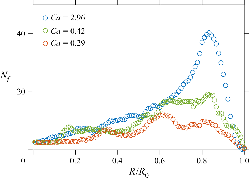
Figure 7. The number of fingers  $N_f$ as a function of the liquid bridge radius $R$ observed in three different experiments. The measurements were performed with $\lambda \approx 0.01$ and $\mathit {Re} \approx 0.1$.
The amplitude of the perturbations at the corresponding conditions,  $\xi =\xi _\star$, $\tau =\tau _\star$, can also be estimated for small capillary numbers:
 \begin{equation} G_\star \approx \delta_0 \exp(0.11 \mathit{Ca}^{1/2} \lambda^{-1}),\quad \mathit{Ca} \ll 1,\quad \mathit{Re} =0. \end{equation}
 Given the approximate estimation of the number of fingers (3.23), the dimensionless parameter  $N_{{max}} \lambda /\mathit {Ca}^{1/2}$ is a function of the Reynolds number if the capillary number is small. In figure 8 this dependency is compared with theoretical predictions based on the numerical computation of the maximum value of the expression for $N_f$ (3.23). The theoretical predictions do not contradict the experiments, although the clear dependence of the number of fingers on the value of the Reynolds number is not that apparent due to the relatively large scatter of data. This scatter can be explained by the fact that in the cases close to the fingering threshold, the amplitude of perturbations is relatively small at the time instant corresponding to $N_f = N_{{max}}$. Therefore, the fingers can only be recognised by the optical system slightly later, when the amplitude magnification is significant. The conditions near the fingering threshold (4.4) are discussed later in this section.
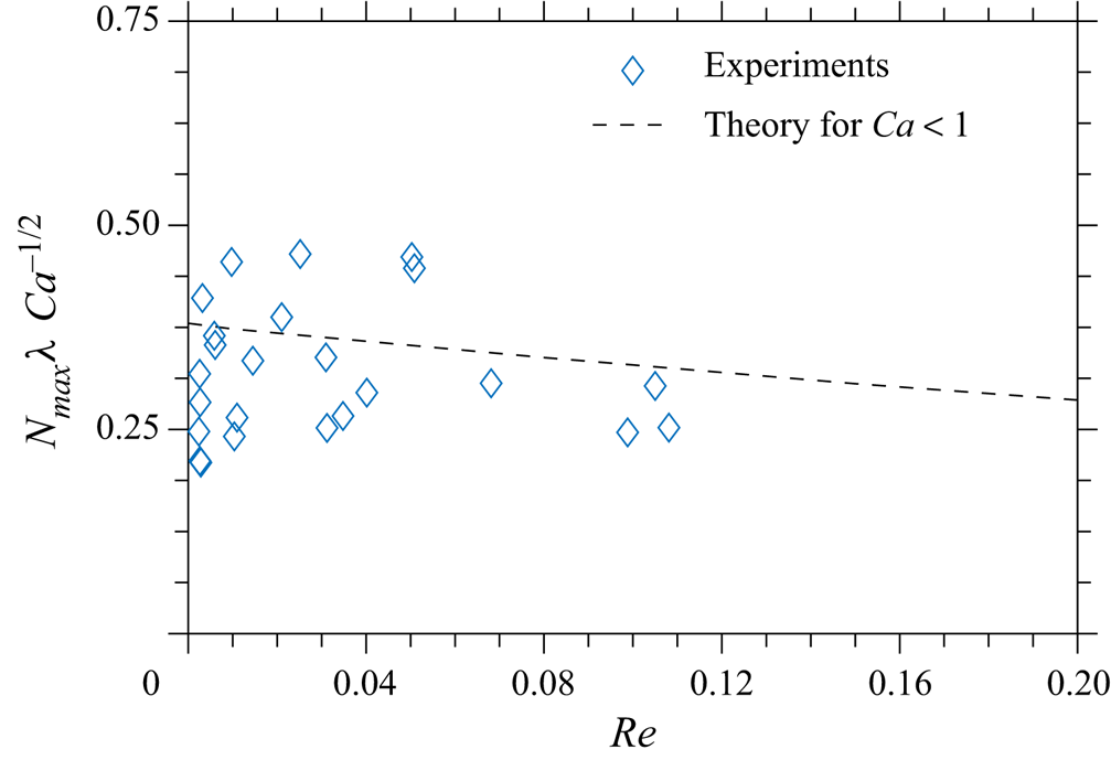
Figure 8. Scaled maximum number of observed fingers  $N_{{max}} \lambda /\mathit {Ca}^{1/2}$ as a function of the Reynolds number.
The approximate solution (3.21) for the most unstable mode, based on the assumption of the smallness of  $\xi _\ast$, does not apply to the cases when the capillary number is not very small. In these cases, a complete numerical solution is required. In this solution the values of $\xi _\ast (\tau )$ for a specific capillary number $\mathit {Ca}$ and Reynolds number are first computed as a point corresponding to the maximum of $\int _0^{\tau } \Omega \,\mathrm {d}\tau$, where $\Omega (\xi ,\tau )$ is defined in (3.18). Then, the maximum number of fingers is computed using (3.22) at the time interval $\tau >0$. The theoretically predicted values of $N_{{\textit{max}}} \lambda$ are determined only by the capillary number and by the Reynolds number. The theoretical predictions of $N_{{max}} \lambda$ are shown in figure 9. As expected, the influence of inertia becomes significant when both the capillary and Reynolds numbers are relatively large.

Figure 9. Computational results of  $N_{{max}} \lambda$ as a function of the capillary number $\mathit {Ca}$ for various Reynolds numbers $\mathit {Re}$. Comparison with theoretical predictions based on the approximate solution.
The significance of the inertial effects in this problem is rather surprising, noting the very small values of Reynolds numbers considered in this study. The main factor governing the fingering process is the pressure gradient at the meniscus interface (3.3), obtained from the base solution. The mechanism of instability caused by the positive normal pressure gradient at the liquid interface is analogous to the Rayleigh–Taylor instability (Chandrasekhar Reference Chandrasekhar2013), where this gradient is caused by gravity or interface acceleration. In the presented case, this term can be written in dimensionless form using (3.8) and (3.18):
 \begin{equation} \frac{p_{0,r}}{\Pi} =\frac{\tau }{(\tau ^{2}+1)^{7/2}} + \frac{\mathit{Re} (1-2 \tau ^{2})}{\sqrt{2} (\tau ^{2}+1)^{5/2}} , \quad \Pi = \frac{\sqrt{a} b \mu }{2 \sqrt{2} H_0^{3/2} \lambda}. \end{equation}
 Function  $p_{0,r}(\tau )/\Pi$ is shown in figure 10 for various values of the Reynolds number. The inertial effects, associated with terms in (4.3), including the Reynolds number, are most pronounced at the very initial stages of bridge stretching, when the substrate velocity (and thus the viscous stresses) is small. This is why, in the case of the liquid bridge stretched by an accelerating substrate, both viscous and inertial effects contribute to the meniscus instability.

Figure 10. The values of the scaled pressure gradient at the meniscus interface  $p_{0, r}/\Pi$ as a function of dimensionless time $\tau$ for various values of the Reynolds number $\mathit {Re}$. The scale for the pressure gradient, $\Pi$, is defined in (4.3).
For the measurements performed on hydrophobic substrates, the number of fingers was estimated correctly, showing that hydrophobicity does not have a significant effect on the fingering instability (see figure 11). As shown in figure 4, the finger patterns start to emerge before the dewetting begins. Following the estimation from Qian & Breuer (Reference Qian and Breuer2011), the time scale for the contact line speed is  $u_{\textit{dewetting}}=\sqrt {\sigma / \rho R}$, which is in our experiments of the order of $10^{-2}$ m s $^{-1}$. The finger formation time scale $\tau =\sqrt {2 H_0/a}$ can be estimated using equation (3.18), which yields $\tau \sim 10^{-4}$ – $10^{-3}$ s. Consequently, the dewetting length for the relevant time scale is of the order of $10^{-6}$– $10^{-5}$ m and therefore too small to affect the fingering instability. The difference between the two time scales provides an approximate validity range of the proposed fingering instability theory. Therefore, the introduced prediction of the number of fingers is in good agreement with substrates of different wetting conditions, as shown in figure 11, as long as the finger formation and dewetting time scales are not of the same order.
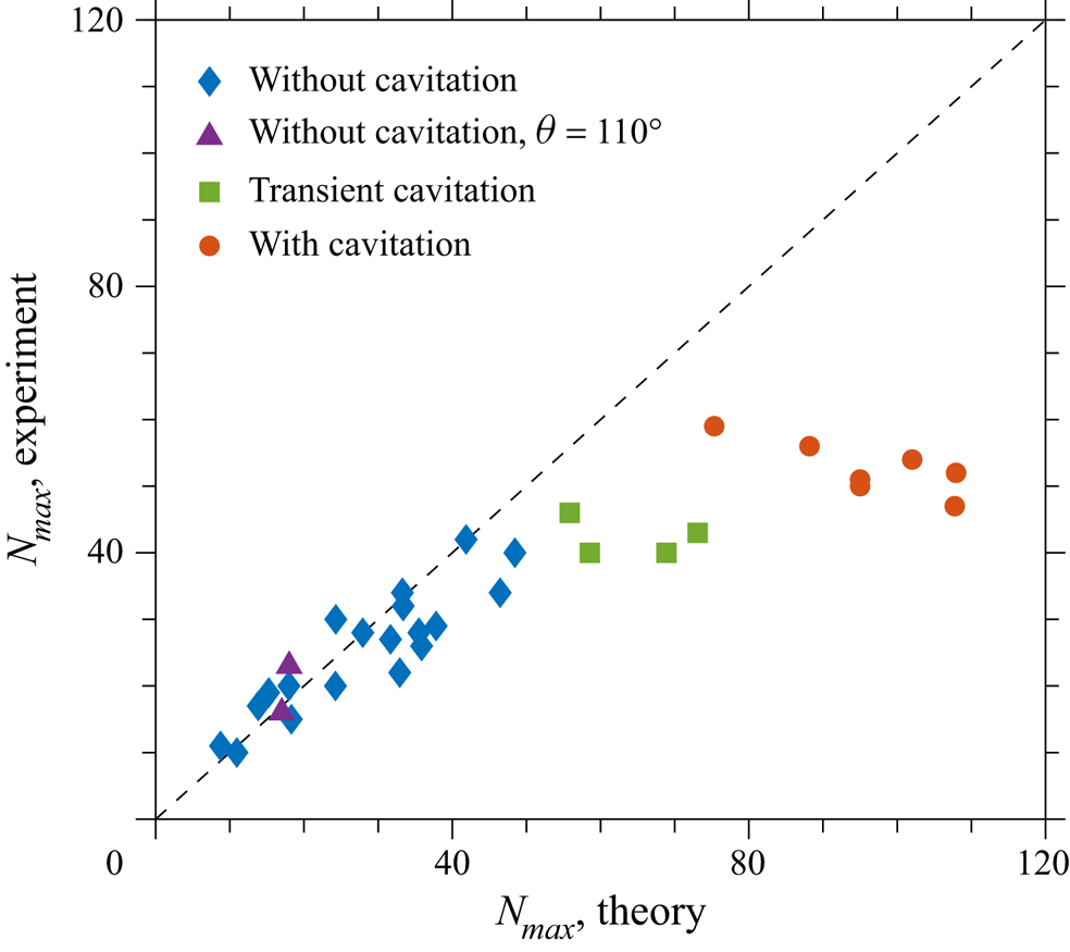
Figure 11. Comparison of the measured and theoretically predicted maximum number of fingers  $N_{{max}}$. The experiments accompanied by cavitation are marked by circles. The static contact angle of the measurements marked as diamonds, rectangles and circles is $\theta _{\textit{static}} = 40^{\circ }$, while that of the measurements marked as triangles is $\theta \approx 110^{\circ }$. The straight dashed line corresponds to perfect agreement between experiment and theory.
The experimental and theoretically predicted values for  $N_{{max}}$ are compared in figure 11. The agreement is rather good for most of the cases. In some instances, however, the number of fingers is overestimated. In all these overestimated experiments, several voids in the liquid bridge have been observed, formed due to cavitation. In some cases these voids quickly expand, leading to the formation of structures resembling Voronoi tessellation, as shown in the examples in figure 12. These cases are marked as liquid bridge stretching with cavitation.

Figure 12. Example of void formation during liquid bridge stretching. The liquid is  $Gly80$. The other experimental parameters are $a=180\ \textrm {m}\ \textrm {s}^{-2}$, $H_0 =60\ {\rm \mu } \textrm {m}$, $\lambda = 0.006$.
Several additional cases have also been observed, marked in figure 13 as transient cavitation. In these cases, a small number of macroscopic voids emerge far from the interface and then disappear after some time when the stresses are relaxed. It is most probable that, in this transitional case, the flow in the stretched bridge is influenced locally, also near the interface, by the nucleation of microbubbles. Even if the size of the bubbles does not exceed the critical diameter of cavity formation, they can still influence the flow near the moving meniscus.
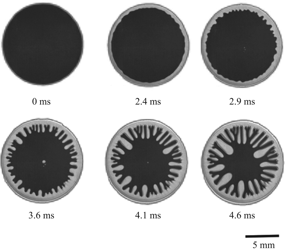
Figure 13. Example of transient cavitation. Several voids are formed in the central part of the liquid bridge and then disappear. The liquid is  $Gly80$. The other experimental parameters are $a=10$ m s $^{-2}$,
  $H_0 =53\ {\rm \
mu }\textrm {m}$,
$H_0 =53\ {\rm \
mu }\textrm {m}$,  $\lambda = 0.006$.
In figure 14 the outcomes of liquid bridge stretching (stable receding of the meniscus without fingering or the emergence of apparent fingering) are shown for various values of  $\lambda$ and $\mathit {Ca}$. It is not always easy to determine the outcome at the limiting cases near the threshold conditions. In this study, fingering is identified if more than five periods of the interface waves can be clearly observed. The condition $N_{{max}}=5$ is used as a criterion for the selection of the experiments leading to fingering. This criterion also allows theoretical prediction of the threshold value $\lambda _{\textit{threshold}}$ for given capillary and Reynolds numbers. As shown in figure 8, the influence of the Reynolds number on the number of the fingers is minor and, to a first approximation, the threshold value $\lambda _{\textit{threshold}}$ is a function only of $\mathit {Ca}$. For small capillary numbers, the threshold value of $\lambda$ can be estimated using the approximate solution (4.1):
 \begin{equation} \lambda_{threshold}\approx 0.076 \sqrt{Ca},\quad \mathit{Ca} \ll 1, \quad \mathit{Re} =0. \end{equation}
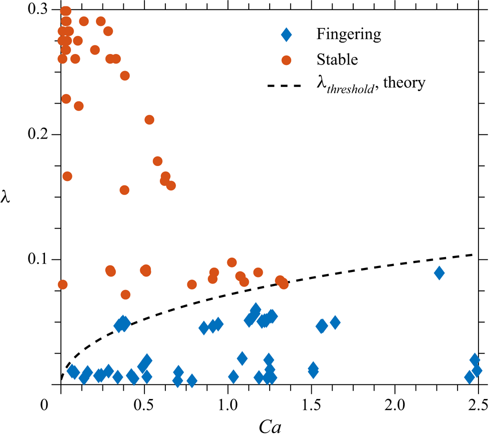
Figure 14. Nomogram for the outcomes of liquid bridge stretching for various values of  $\lambda$ and capillary number $\mathit {Ca}$. The threshold for bridge fingering is obtained from the full computations for $Re=0$ of $\lambda _{\textit{threshold}}$, corresponding to the condition $N_{{max}}=5$. The approximate solution (4.4) is also shown on the graph, but it is indistinguishable from the results of full computations for $\mathit {Ca}<1$.
It is interesting to note that in the limit  $\mathit {Re}=0$, the same scaling as in (4.4), namely $\lambda _{threshold}\sim \sqrt {\mathit {Ca}}$, corresponds also to a certain amplitude $G_{\textit{threshold}}\approx 1.7\delta _0$ of the shape perturbations $\delta (y,t)$, where $\delta _0$ is the initial shape disturbance. This relation can be obtained from (4.2). Since the initial disturbance $\delta$ is very small, the perturbations of the amplitude $G_{threshold}$ cannot be resolved with the optical system. Note, however, that $G_{threshold}$ characterises the amplitude of the perturbations at the predicted time $\tau = \tau _\star$, corresponding to the maximum number of fingers. This amplitude continues to grow nearly exponentially in time. This is why in the cases close to the threshold, the fingers can be recognised at times slightly larger than $\tau _\star$ and thus at radii close to $R/R_0 \approx 0.8$, as shown, for example, for the case $\mathit {Ca} = 0.29$ in figure 7.
Therefore, both conditions, a certain number of fingers and a certain amplitude of the disturbances, can be used as conditions for the observable generation of fingers.
5. Conclusion
In this study, the pattern formation in a liquid bridge stretched by an accelerating substrate is investigated experimentally and modelled theoretically. The maximum number of fingers is measured for a large range of liquid viscosities, gap widths and substrate accelerations.
The process of finger formation is studied using linear stability analysis for small perturbations of the liquid bridge shape. The theory accounts for the viscous stresses, capillary forces and inertial effects. The model is developed for a single-sided accelerated substrate. It allows calculations of the amplitude of a certain wavelength on the bridge surface over time as long as  $\lambda \ll 1$ and the two-dimensional approximation applies to the flow field. Consequently, a prediction is derived for the number of fingers. The agreement with observations is good, despite the fact that no adjustable parameters have been introduced into the model. The prediction is, however, only applicable if no cavitation occurs. For experimental cases where cavitation occurs, the theory overestimates the number of fingers.
A criterion  $\lambda _{threshold}\approx 0.076 \sqrt {\mathit {Ca}}$ has been obtained for the onset of fingering instability. The fingering assumed a certain number of observable fingers. For lower numbers $N_{{max}}<5$, the instability is perceived as the loss of the asymmetric shape, but not as fingering. For $N_{{max}}<1$ the flow should be stable.
An alternative condition for fingering, namely the threshold value for the amplitude of perturbations, leads to the same scaling for the threshold conditions:  $\lambda _{threshold}\sim \sqrt {\mathit {Ca}}$.
Acknowledgments
The authors gratefully acknowledge the financial support of the German Research Foundation (DFG) within the Collaborative Research Centre 1194 ‘Interaction of Transport and Wetting Processes’, Project A03. The authors would like to thank the Institute for Nano- and Microfluidics at Technische Universität Darmstadt from Steffen Hardt, especially Maximilian Hartmann, for providing silanised substrates for this study.
Declaration of interests
The authors report no conflict of interest.


 Open access