


1 Introduction
Continuous particle-driven gravity currents frequently occur in nature and industry. In nature, examples include pyroclastic flows issuing from volcanoes, sustained turbidity currents and the continuous discharge of particles into lakes and oceans by sediment-laden rivers (Bonnecaze, Huppert & Lister Reference Bonnecaze, Huppert and Lister1993; Middleton Reference Middleton1993; Simpson Reference Simpson1999; Ungarish Reference Ungarish2009; Steel et al. Reference Steel, Simms, Warrick and Yokoyama2016). In the oil and gas industry, the process industry and in water treatment facilities, separators are employed to split continuous streams of multiphase mixtures into their single-phase components (DeRooij Reference DeRooij1999). Understanding the run-out distance and sedimentation from these flows as well as the fate of the host fluid is important to optimise industrial equipment and to assess the hazards posed by naturally occurring particle-driven currents, especially since contaminants on the particles may become dissolved in the host fluid.
In the sedimentology literature, there is a wealth of papers exploring the sedimentation of particles in settling columns (Kynch Reference Kynch1952; Davis & Acrivos Reference Davis and Acrivos1985), and often the effects of hindered settling lead to dispersal of the sedimentation front (Blanchette & Bush Reference Blanchette and Bush2005; Guazzelli & Hinch Reference Guazzelli and Hinch2011).
There is also a significant literature exploring the dynamics of particle-laden gravity currents, arising from the original work of von Kármán (Reference Karman1940) and Benjamin (Reference Benjamin1968). Many authors have explored the dynamics of finite-volume gravity currents produced by the release of a fixed volume of fluid from a lock gate. Models of these flows often assume that the flow maintains a constant volume (Bonnecaze et al.
Reference Bonnecaze, Huppert and Lister1993; Huppert Reference Huppert1998; Simpson Reference Simpson1999; Huppert Reference Huppert2006; Ungarish Reference Ungarish2009). For such particle-laden gravity currents, the concentration is then assumed to decrease through sedimentation from the base of the flow, while the current is often assumed to remain well mixed at each position along the flow and the effects of any sedimentation front are ignored (Bonnecaze et al.
Reference Bonnecaze, Huppert and Lister1993). These simplifications have been successful in developing models to describe the position of the nose of the current as a function of time in the case that the current speed far exceeds the particle settling velocity, $u(x)\gg u_{fall}$
. Given that sedimentation fronts do develop in settling columns, it is of interest to explore if there are conditions under which a sedimentation front develops in gravity-driven flows, and to explore the fate of the host fluid as the particles sediment. In our investigation, the density of the interstitial host fluid corresponds to the density of the ambient fluid, so that any reduction in buoyancy of the gravity current is attributed to the sedimentation of particles on the floor. We note that if the density of the host fluid exceeds the density of the ambient fluid, the overall density and thus the velocity of the gravity current would increase. The host fluid would continue to travel as a single-phase gravity current after the particles have sedimented. Conversely, if the interstitial host fluid is less dense than the ambient fluid, the overall buoyancy of the gravity current would be reduced and the gravity current would lose buoyancy through the sedimentation of particles as well as through the escape of host liquid at the top of the gravity current. Depending on the magnitude of the density difference between host fluid and ambient fluid, and the size and density of the particles, the lofting interstitial fluid may lift particles up from the gravity current (Steel et al.
Reference Steel, Buttles, Simms, Mohrig and Meiburg2017). This complication is beyond the scope of the present study.
$u(x)\gg u_{fall}$
. Given that sedimentation fronts do develop in settling columns, it is of interest to explore if there are conditions under which a sedimentation front develops in gravity-driven flows, and to explore the fate of the host fluid as the particles sediment. In our investigation, the density of the interstitial host fluid corresponds to the density of the ambient fluid, so that any reduction in buoyancy of the gravity current is attributed to the sedimentation of particles on the floor. We note that if the density of the host fluid exceeds the density of the ambient fluid, the overall density and thus the velocity of the gravity current would increase. The host fluid would continue to travel as a single-phase gravity current after the particles have sedimented. Conversely, if the interstitial host fluid is less dense than the ambient fluid, the overall buoyancy of the gravity current would be reduced and the gravity current would lose buoyancy through the sedimentation of particles as well as through the escape of host liquid at the top of the gravity current. Depending on the magnitude of the density difference between host fluid and ambient fluid, and the size and density of the particles, the lofting interstitial fluid may lift particles up from the gravity current (Steel et al.
Reference Steel, Buttles, Simms, Mohrig and Meiburg2017). This complication is beyond the scope of the present study.
We have chosen to study the dynamics of steady particle-driven gravity currents which are sustained by a maintained source of particle-laden fluid. We explore the conditions under which a sedimentation front develops on the upper surface of the gravity current, and we assess the impact of this on the evolution of the mass and momentum flux of the flow. In our investigation, we assume that the Shields parameter of the flow is sufficiently small, so that the re-suspension of particles from the bed can be neglected (cf. Eames et al.
Reference Eames, Hogg, Gething and Dalziel2001). First, we present a series of experiments in which steady, particle-driven gravity currents develop from the collapse of turbulent multiphase fountains. This source condition allows for the supply of a continuous volume flux without imposing an initial horizontal momentum to the flow. We measure the depth of the current as a function of position and we use finite pulses of dye in the source fluid to determine the fate of the fluid as it moves through the current. We also develop a quantitative model for the conservation of the fluxes of volume, momentum and buoyancy. This model accounts for a possible sedimentation front, and, by comparison with our experimental data, we propose that the effective speed of this front decreases as the ratio of the current speed to the fall speed of the particles, $S$
, increases. We consider the implications of our model for the dynamics of particle-laden gravity currents in industry and nature.
$S$
, increases. We consider the implications of our model for the dynamics of particle-laden gravity currents in industry and nature.
2 Experimental method
Particle-driven gravity currents were generated by issuing a mixture of fresh water and mono-dispersed silicon-carbide particles through a nozzle upwards 10 cm from the end of a Perspex tank $L_{tank}=3~\text{m}$
long, 40 cm high and 15 cm wide, initially filled with fresh water. The dense, particle-laden jet exiting through the nozzle decelerates owing to its negative buoyancy and the entrainment of ambient liquid. The jet eventually comes to rest and collapses, thereby forming a turbulent multiphase fountain with a source Reynolds number of approximately 2500. This source Reynolds number is based on the density of the injected fluid,
$L_{tank}=3~\text{m}$
long, 40 cm high and 15 cm wide, initially filled with fresh water. The dense, particle-laden jet exiting through the nozzle decelerates owing to its negative buoyancy and the entrainment of ambient liquid. The jet eventually comes to rest and collapses, thereby forming a turbulent multiphase fountain with a source Reynolds number of approximately 2500. This source Reynolds number is based on the density of the injected fluid, $\unicode[STIX]{x1D70C}_{S}$
, and the nozzle diameter,
$\unicode[STIX]{x1D70C}_{S}$
, and the nozzle diameter, $d_{S}=8.6~\text{mm}$
, as a length scale,
$d_{S}=8.6~\text{mm}$
, as a length scale,
 $$\begin{eqnarray}Re_{S}=\frac{\unicode[STIX]{x1D70C}_{S}u_{S}d_{S}}{\unicode[STIX]{x1D707}_{W}},\end{eqnarray}$$
where $\unicode[STIX]{x1D707}_{W}\approx 1~\text{mPa}~\text{s}$
is the dynamic viscosity of water at room temperature and
$\unicode[STIX]{x1D707}_{W}\approx 1~\text{mPa}~\text{s}$
is the dynamic viscosity of water at room temperature and $u_{S}$
is the nozzle exit velocity. The density of the source fluid,
$u_{S}$
is the nozzle exit velocity. The density of the source fluid, $\unicode[STIX]{x1D70C}_{S}$
, is proportional to the source concentration of particles,
$\unicode[STIX]{x1D70C}_{S}$
, is proportional to the source concentration of particles, $C_{S}$
.
$C_{S}$
.
A schematic of the experimental set-up is shown in figure 1. After an initial transient, the current reaches a steady state. In this paper we present a set of 35 experiments, 24 of which were run with a single fountain source. The corresponding experimental set-up is shown in figure 1(a). The second schematic in this panel is a top view of the tank, focusing on the nozzle section to illustrate the positioning of the nozzle. A further set of 8 experiments were run with two fountain sources distributed evenly in the spanwise direction of the tank to double the volume flux. The corresponding experimental set-up is shown in figure 1(b). These experiments are marked with an asterisk (*) in table 1. Three additional experiments were run with a plume source, directed downwards and placed 12.5 cm above the base of the tank. Figure 1(c) contains a schematic of this experimental set-up. These experiments are marked with two asterisks (**). In three experiments, the gravity current did not sediment the particle load prior to reaching the end of the tank, and so a steady state was not reached. These experiments are marked with three asterisks (***). The source liquid, a mixture of fresh water and Carborex silicon-carbide particles produced by Washington Mills, was pumped with a Watson Marlow peristaltic pump. The particles have diameters between 13 and $63~\unicode[STIX]{x03BC}\text{m}$
. The concentration at the source of the fountain was kept between 20 and 80 grams of particles per litre of water. This concentration was further reduced by dilution in the fountain, resulting in gravity currents with initial Reynolds numbers between 500 and 1600. The initial Reynolds number of the gravity current is based on the density of fluid at the onset of the gravity current,
$63~\unicode[STIX]{x03BC}\text{m}$
. The concentration at the source of the fountain was kept between 20 and 80 grams of particles per litre of water. This concentration was further reduced by dilution in the fountain, resulting in gravity currents with initial Reynolds numbers between 500 and 1600. The initial Reynolds number of the gravity current is based on the density of fluid at the onset of the gravity current, $\unicode[STIX]{x1D70C}_{0}$
, and the initial current height,
$\unicode[STIX]{x1D70C}_{0}$
, and the initial current height, $h_{0}$
, as a length scale,
$h_{0}$
, as a length scale,
 $$\begin{eqnarray}Re_{0}=\frac{\unicode[STIX]{x1D70C}_{0}u_{0}h_{0}}{\unicode[STIX]{x1D707}_{W}},\end{eqnarray}$$
where $u_{0}$
is the initial velocity of the gravity current. Please refer to § 4 for a detailed discussion of the initial values of current height, density and velocity. The source Reynolds number,
$u_{0}$
is the initial velocity of the gravity current. Please refer to § 4 for a detailed discussion of the initial values of current height, density and velocity. The source Reynolds number, $Re_{S}$
(2.1), is calculated per nozzle. For the double fountain source, however, the initial Reynolds number of the current,
$Re_{S}$
(2.1), is calculated per nozzle. For the double fountain source, however, the initial Reynolds number of the current, $Re_{0}$
(2.2), is calculated based on the added flow rates from the two sources forming the gravity current.
$Re_{0}$
(2.2), is calculated based on the added flow rates from the two sources forming the gravity current.
An electroluminescent light sheet was placed behind the tank to provide uniform illumination. Images were recorded with a JAI 5000-C camera. The videos, 6.25 min in length, have a frame rate of 4 Hz. The steady-state shape of the gravity currents was extracted by time averaging over the last 2 min of the experiments.
In the experiments marked with a subscript $b$
in table 1 a burst of red dye was added to the source liquid. The density difference between this water-based dye and the ambient fresh water is much smaller than the density difference between the particle-laden water and the fresh water, so that the effects of the dye on the flow are negligible.
$b$
in table 1 a burst of red dye was added to the source liquid. The density difference between this water-based dye and the ambient fresh water is much smaller than the density difference between the particle-laden water and the fresh water, so that the effects of the dye on the flow are negligible.

Figure 1. Two-dimensional schematic of the experimental apparatus and cartoon of the transition of the flow from a turbulent fountain or plume into a particle-driven gravity current. The second cartoon in each panel is a top view of the tank, focussing on the nozzle section to illustrate the nozzle arrangement on a horizontal plane. (a) Single fountain source, (b) double fountain source and (c) single plume source.
Table 1. Table with source conditions: number of the experiment (Exp.), particle diameter ( $d_{P}$
), particle fall speed (
$d_{P}$
), particle fall speed ( $u_{fall}$
), particle concentration supplied through nozzle (
$u_{fall}$
), particle concentration supplied through nozzle ( $C_{S}$
), volume flux supplied through nozzle (
$C_{S}$
), volume flux supplied through nozzle ( $Q_{S}$
), source Froude number of the fountain (
$Q_{S}$
), source Froude number of the fountain ( $Fr_{S}$
), initial volume flux feeding the gravity current (
$Fr_{S}$
), initial volume flux feeding the gravity current ( $Q_{0}$
), initial velocity of the gravity current (
$Q_{0}$
), initial velocity of the gravity current ( $u_{0}$
), ratio of fluid velocity to particle settling velocity (
$u_{0}$
), ratio of fluid velocity to particle settling velocity ( $S$
) and initial Reynolds number of the current (
$S$
) and initial Reynolds number of the current ( $Re_{0}$
). In experiments marked with (*) the source was comprised of two nozzles. In experiments marked with (**) the mixture was issued into the tank as a plume (directed downwards), positioned 12.5 cm above the floor. In experiments marked with (***), the currents reached the end of the 3 m flume tank. In experiments with subscript
$Re_{0}$
). In experiments marked with (*) the source was comprised of two nozzles. In experiments marked with (**) the mixture was issued into the tank as a plume (directed downwards), positioned 12.5 cm above the floor. In experiments marked with (***), the currents reached the end of the 3 m flume tank. In experiments with subscript $b$
a burst of red dye was added to the source liquid in steady state. These experiments were run in a tank 150 cm long and 10 cm deep. The value for
$b$
a burst of red dye was added to the source liquid in steady state. These experiments were run in a tank 150 cm long and 10 cm deep. The value for $Q_{0}$
was computed from (4.4) and the initial velocity was obtained via the relation
$Q_{0}$
was computed from (4.4) and the initial velocity was obtained via the relation $u_{0}=\sqrt{g_{0}^{\prime }h_{0}}$
.
$u_{0}=\sqrt{g_{0}^{\prime }h_{0}}$
.

3 Experimental observations
In the experiments we have systematically varied the size and concentration of the particles, the source fluid volume flux and the orientation of the source (single fountain source, double fountain source, plume source).
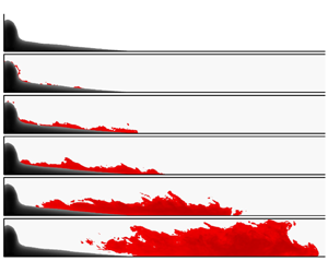
Figure 2(a) shows an instantaneous image of a gravity current (Exp. 6) in steady state. A dark colour indicates a high concentration of particles. The image shows the multiphase fountain to the left. This feeds the gravity current which gradually thins out over approximately 150 cm. Figure 2(b) shows a two minute time-averaged shape of the gravity current in false colour. Dark blue indicates a high concentration of particles, red denotes the absence of particles. This time-averaged shape smooths the fluctuations in depth of the current and corresponds to the steady mean shape of the gravity current. The fluctuations, visible in panel (a), lead to a diffuse front in the time-averaged image. Figure 2(c–e) shows time-series images of the three vertical lines shown in (a,b). We interpret the oscillations around a mean depth as the result of apparent turbulent fluctuations in the flow. The mean depth and the particle concentration decrease from panel (c) to panel (e) corresponding to the change in the gravity current as it moves downstream.
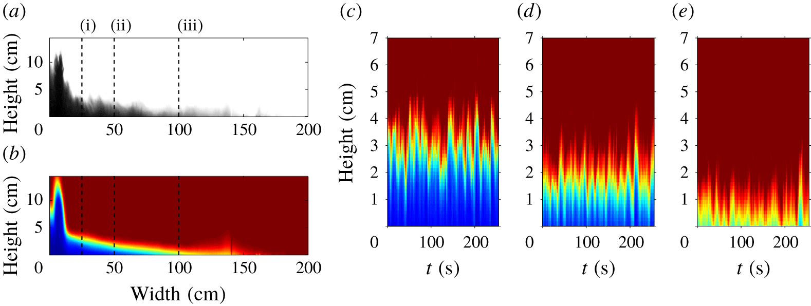
Figure 2. (a) Instantaneous image of the gravity current (Exp. 6 in table 1). (b) False-colour image of the time-averaged, steady-state shape of the current. Blue colour denotes a high concentration of particles, red colour denotes the absence of particles. (c–e) False-colour time-series images at the locations marked by columns (i), (ii) and (iii) in (a,b).
In experiments 31–35 we added a finite volume of red dye to the source liquid supplied through the nozzle once the steady current had become established. As the fluid moves along the current, it may be seen that in experiments 31–34 some of the dyed liquid separates from the upper surface of the current (see figure 3(a–f) for experiment 33). In panel (a) only the time-averaged shape of the fountain and gravity current (in dark grey) is visible. This figure indicates that fluid detrains from the gravity current into the environment as the particles sediment from the flow. Panels (e,f) highlight that the dyed fluid continues to travel along the tank, implying that this liquid also carries momentum away from the gravity current. Panel (g) corresponds to panel (d), but the instantaneous outline of the gravity current is shown, rather than the time-averaged profile.

Figure 3. (a) Visualisation of the time-averaged steady-state shape of the gravity current in grey. (b–f) A burst of red dye was added to the source liquid to investigate the separation of the source liquid from the gravity current. Red dye emerges above the current, along the entire length of the current. This dyed liquid continues to propagate owing to its residual momentum. (g) Instantaneous shape of the gravity current corresponding to panel (d).
In figure 4(a) we show the thickness versus distance of 27 experiments. We do not include the three experiments which reach the end of the flume tank. The colour coding indicates the value of the dimensionless settling parameter, $S$
,
$S$
,
 $$\begin{eqnarray}S=\frac{u_{0}}{u_{fall}},\end{eqnarray}$$
where $u_{0}$
is the initial velocity of the gravity current and
$u_{0}$
is the initial velocity of the gravity current and $u_{fall}$
is the terminal fall speed of the particles. Please refer to (4.5) for the exact definition of
$u_{fall}$
is the terminal fall speed of the particles. Please refer to (4.5) for the exact definition of $u_{fall}$
.
$u_{fall}$
.
Dark blue corresponds to $S\approx 5$
, and dark red corresponds to
$S\approx 5$
, and dark red corresponds to $S\approx 30$
. This plot shows that the run-out distance and the total area occupied by the gravity current increase for larger values of
$S\approx 30$
. This plot shows that the run-out distance and the total area occupied by the gravity current increase for larger values of $S$
. It has previously been shown that the parameter
$S$
. It has previously been shown that the parameter $S$
is crucial for describing the dynamics of transient particle-laden gravity currents produced by a finite release of fluid (Bonnecaze et al.
Reference Bonnecaze, Huppert and Lister1993). The depth on the
$S$
is crucial for describing the dynamics of transient particle-laden gravity currents produced by a finite release of fluid (Bonnecaze et al.
Reference Bonnecaze, Huppert and Lister1993). The depth on the $y$
-axis and the distance travelled on the
$y$
-axis and the distance travelled on the $x$
-axis are both normalised by the initial depth,
$x$
-axis are both normalised by the initial depth, $h_{0}$
. In § 4 we give a detailed description of the initial velocity
$h_{0}$
. In § 4 we give a detailed description of the initial velocity $u_{0}$
and depth
$u_{0}$
and depth $h_{0}$
.
$h_{0}$
.
We note that in experiment 35, obtained for $S=126$
, we did not observe a reduction in height of the gravity current along the entire length of the tank and the dye remained confined to the gravity current.
$S=126$
, we did not observe a reduction in height of the gravity current along the entire length of the tank and the dye remained confined to the gravity current.

Figure 4. (a) Plot of dimensionless depth as a function of dimensionless distance from the source for 27 experiments (experiments marked with (***) were excluded). The depth and the horizontal distance are normalised by $h_{0}$
. (b) Cartoon of a particle-laden gravity current in steady state. The particle concentration,
$h_{0}$
. (b) Cartoon of a particle-laden gravity current in steady state. The particle concentration, $C(x)$
, the volume flux,
$C(x)$
, the volume flux, $q(x)$
, and the depth of the current,
$q(x)$
, and the depth of the current, $h(x)$
, decrease with distance from the source.
$h(x)$
, decrease with distance from the source.
Figure 4(b) shows a cartoon describing the processes within the gravity current. The current is fed by the fountain which supplies an initial volume flux per unit width, $q_{0}=u_{0}h_{0}$
, as well as an initial particle volume fraction,
$q_{0}=u_{0}h_{0}$
, as well as an initial particle volume fraction, $C_{0}$
. As particles settle there is a reduction in depth of the current, and some deposition of particles at the base of the tank. The reduction in depth releases some of the fluid from the upper surface of the current. However, the apparent turbulent fluctuations (figure 2) lead to some mixing near this interface so that the rate of decrease of depth of the current is smaller than the fall speed of the particles. These turbulent fluctuations are likely to arise owing to the small density gradient between the top of the propagating gravity current and the ambient as the particles begin to settle from the top of the gravity current. This shear-driven mixing, in turn, leads to a reduction in the speed of the sedimentation front to values smaller than the fall speed of the particles. Owing to the low concentration of particles (
$C_{0}$
. As particles settle there is a reduction in depth of the current, and some deposition of particles at the base of the tank. The reduction in depth releases some of the fluid from the upper surface of the current. However, the apparent turbulent fluctuations (figure 2) lead to some mixing near this interface so that the rate of decrease of depth of the current is smaller than the fall speed of the particles. These turbulent fluctuations are likely to arise owing to the small density gradient between the top of the propagating gravity current and the ambient as the particles begin to settle from the top of the gravity current. This shear-driven mixing, in turn, leads to a reduction in the speed of the sedimentation front to values smaller than the fall speed of the particles. Owing to the low concentration of particles ( $C_{0}<0.5\,\%$
by volume) it is likely that convective mixing, caused by convective particle settling, is negligible (Hoyal, Bursik & Atkinson Reference Hoyal, Bursik and Atkinson1999). Owing to the change in density of the upper parts of the current associated with the sedimentation, the entrainment process is different to the mixing of ambient fluid into continuous single-phase gravity currents. In a single-phase gravity current, mixing occurs predominantly near the head of the current, while the density gradient between the tail of the gravity current and the ambient limits the mixing behind the head (Sher & Woods Reference Sher and Woods2017).
$C_{0}<0.5\,\%$
by volume) it is likely that convective mixing, caused by convective particle settling, is negligible (Hoyal, Bursik & Atkinson Reference Hoyal, Bursik and Atkinson1999). Owing to the change in density of the upper parts of the current associated with the sedimentation, the entrainment process is different to the mixing of ambient fluid into continuous single-phase gravity currents. In a single-phase gravity current, mixing occurs predominantly near the head of the current, while the density gradient between the tail of the gravity current and the ambient limits the mixing behind the head (Sher & Woods Reference Sher and Woods2017).
From the contours of the gravity currents displayed in figure 4(a) one can extract the run-out distance of the gravity current, $L$
, defined as the horizontal distance from the source, at which
$L$
, defined as the horizontal distance from the source, at which $h=h_{0}$
, to the point where
$h=h_{0}$
, to the point where $h=0$
. These contours were obtained from the time-averaged gravity current profiles (cf. figure 2
b). In estimating the run-out distance, there is some variability in the exact distance owing to the fluctuations in the flow; we have included some estimate of this variability by comparing the location of the run-out lengths estimated from the time-averaged images of the flow, using the light-intensity contour of 0.4, with error bars representing the distances reached by light intensity contours of 0.3 and 0.5 (see figure 2). The run-out distance,
$h=0$
. These contours were obtained from the time-averaged gravity current profiles (cf. figure 2
b). In estimating the run-out distance, there is some variability in the exact distance owing to the fluctuations in the flow; we have included some estimate of this variability by comparing the location of the run-out lengths estimated from the time-averaged images of the flow, using the light-intensity contour of 0.4, with error bars representing the distances reached by light intensity contours of 0.3 and 0.5 (see figure 2). The run-out distance, $L$
, normalised by the initial height,
$L$
, normalised by the initial height, $h_{0}$
, is shown as a function of
$h_{0}$
, is shown as a function of $S$
in figure 5(a), demonstrating that the run-out length increases as either the initial current speed increases or the particle fall speed decreases. The dash-dotted line in this figure corresponds to a power-law best fit of our experimental data in the form
$S$
in figure 5(a), demonstrating that the run-out length increases as either the initial current speed increases or the particle fall speed decreases. The dash-dotted line in this figure corresponds to a power-law best fit of our experimental data in the form
 $$\begin{eqnarray}\frac{L}{h_{0}}=aS^{b},\end{eqnarray}$$
with $a=0.048$
and
$a=0.048$
and $b=2.2$
. The coefficient of determination,
$b=2.2$
. The coefficient of determination, $R^{2}$
, of this fit is 0.92.
$R^{2}$
, of this fit is 0.92.

Figure 5. (a) Plot of experimental run-out length of the gravity current, $L$
, normalised by the initial height of the gravity current,
$L$
, normalised by the initial height of the gravity current, $h_{0}$
, as a function of
$h_{0}$
, as a function of $S=u_{0}/u_{fall}$
. (b) Plot of the ratio of fall time,
$S=u_{0}/u_{fall}$
. (b) Plot of the ratio of fall time, $\unicode[STIX]{x1D70F}_{fall}=h_{0}/u_{fall}$
and travel time,
$\unicode[STIX]{x1D70F}_{fall}=h_{0}/u_{fall}$
and travel time, $\unicode[STIX]{x1D70F}_{travel}=L/u_{0}$
as a function of
$\unicode[STIX]{x1D70F}_{travel}=L/u_{0}$
as a function of $S$
. Circles correspond to experiments marked with (***).The dash-dotted line in both panels describes a power-law best fit, defined in the legend.
$S$
. Circles correspond to experiments marked with (***).The dash-dotted line in both panels describes a power-law best fit, defined in the legend.
For simple settling, the time required for a particle to fall from the top of the gravity current to the floor is $\unicode[STIX]{x1D70F}_{fall}=h_{0}/u_{fall}$
, while we expect the travel time of the particle from the source to the end of the gravity current to scale as
$\unicode[STIX]{x1D70F}_{fall}=h_{0}/u_{fall}$
, while we expect the travel time of the particle from the source to the end of the gravity current to scale as $\unicode[STIX]{x1D70F}_{travel}=L/u_{0}$
. In figure 5(b) we plot the ratio of
$\unicode[STIX]{x1D70F}_{travel}=L/u_{0}$
. In figure 5(b) we plot the ratio of $\unicode[STIX]{x1D70F}_{fall}$
and
$\unicode[STIX]{x1D70F}_{fall}$
and $\unicode[STIX]{x1D70F}_{travel}$
, measured in our experiments, as a function of
$\unicode[STIX]{x1D70F}_{travel}$
, measured in our experiments, as a function of $S$
, and we observe that this ratio decreases for larger values of
$S$
, and we observe that this ratio decreases for larger values of $S$
. We note that for
$S$
. We note that for $S>40$
, we do not in fact observe a reduction in depth over the entire length of the 3 metre flume tank (experiments marked with (***)). These data suggest that the effective descent speed of the sedimentation front,
$S>40$
, we do not in fact observe a reduction in depth over the entire length of the 3 metre flume tank (experiments marked with (***)). These data suggest that the effective descent speed of the sedimentation front, $u_{front}$
, decreases relative to the fall speed of individual particles,
$u_{front}$
, decreases relative to the fall speed of individual particles, $u_{fall}$
, as
$u_{fall}$
, as $S$
increases. We hypothesise that the reduction of the apparent fall speed of the sedimentation front results from the increasing importance of the mixing near the top surface of the current as the current speed increases to values far in excess of the settling speed of the particles (cf. Cardoso & Woods Reference Cardoso and Woods1995). The dash-dotted line corresponds to the power-law best fit shown in panel (a). On this plot, this best fit has the form
$S$
increases. We hypothesise that the reduction of the apparent fall speed of the sedimentation front results from the increasing importance of the mixing near the top surface of the current as the current speed increases to values far in excess of the settling speed of the particles (cf. Cardoso & Woods Reference Cardoso and Woods1995). The dash-dotted line corresponds to the power-law best fit shown in panel (a). On this plot, this best fit has the form
 $$\begin{eqnarray}\frac{\unicode[STIX]{x1D70F}_{fall}}{\unicode[STIX]{x1D70F}_{travel}}=\frac{Sh_{0}}{L}=\frac{1}{a}S^{1-b}.\end{eqnarray}$$
This best fit has only been plotted over the range for which it has been validated experimentally (see panel a) and it is in good agreement with the experimental data.
4 Theoretical model
4.1 Initial conditions
The source fluxes of volume, momentum and buoyancy, $Q_{S}$
,
$Q_{S}$
, $M_{S}$
and
$M_{S}$
and $B_{S}$
issuing through the nozzle can be used to construct a source Froude number for the fountain,
$B_{S}$
issuing through the nozzle can be used to construct a source Froude number for the fountain,
 $$\begin{eqnarray}Fr_{s}=\frac{(M_{S}/\unicode[STIX]{x03C0})^{5/4}}{(Q_{S}/\unicode[STIX]{x03C0})(B_{S}/\unicode[STIX]{x03C0})^{1/2}}=\frac{u_{S}}{\sqrt{b_{S}g_{S}^{\prime }}},\end{eqnarray}$$
where $u_{S}$
is the nozzle exit velocity of the mixture,
$u_{S}$
is the nozzle exit velocity of the mixture, $b_{S}=4.3~\text{mm}$
is the nozzle radius and
$b_{S}=4.3~\text{mm}$
is the nozzle radius and $g_{S}^{\prime }$
is the reduced gravity at the source (Hunt & Burridge Reference Hunt and Burridge2015). The source momentum flux is
$g_{S}^{\prime }$
is the reduced gravity at the source (Hunt & Burridge Reference Hunt and Burridge2015). The source momentum flux is
 $$\begin{eqnarray}M_{s}=Q_{S}u_{S}=\unicode[STIX]{x03C0}b_{S}^{2}u_{S}^{2},\end{eqnarray}$$
and the source buoyancy flux is
 $$\begin{eqnarray}B_{s}=Q_{S}g_{S}^{\prime }=\unicode[STIX]{x03C0}b_{S}^{2}u_{S}g_{S}^{\prime }.\end{eqnarray}$$
In our experiments, the terminal particle fall speed, $u_{fall}$
, is small compared to the characteristic velocity of the fountain (cf. appendix A), so that the fountain behaves as an analogous single-phase fountain (Mingotti & Woods Reference Mingotti and Woods2016). We employ an empirical correlation developed through careful experiments by Burridge & Hunt (Reference Burridge and Hunt2016) to estimate the entrainment into the fountain based on the Froude number, leading to the estimate for the volume flux feeding the gravity current
$u_{fall}$
, is small compared to the characteristic velocity of the fountain (cf. appendix A), so that the fountain behaves as an analogous single-phase fountain (Mingotti & Woods Reference Mingotti and Woods2016). We employ an empirical correlation developed through careful experiments by Burridge & Hunt (Reference Burridge and Hunt2016) to estimate the entrainment into the fountain based on the Froude number, leading to the estimate for the volume flux feeding the gravity current
 $$\begin{eqnarray}Q_{0}=0.71(Fr_{s}+1)Q_{s}.\end{eqnarray}$$
In the appendix A, we present a further set of experiments in which we measure the entrainment into the turbulent fountains analogous to those generated in our experiment. These additional experiments are conducted first in an unconfined environment, and second in a confined tank of width and depth 17 cm. These experiments confirm that the entrainment into the fountain is not hindered by the presence of the walls of the flume tank in the present experimental set-up, so that (4.4) serves as a good approximation for the initial volume flux of the gravity current. In the three experiments run with plume sources (marked with (**) in table 1) the classical solutions for turbulent plumes were employed to estimate the analogous flux (Morton, Taylor & Turner Reference Morton, Taylor and Turner1956). We assume that there is no particle settling within the area occupied by the fountain, owing to the much higher flow speed of the fountain as compared to the particle settling speed, so the buoyancy flux supplied to the gravity current from the fountain is assumed to equal the buoyancy flux supplied to the tank by the pump. The initial reduced gravity of the current is thus $g_{0}^{\prime }=g_{s}^{\prime }Q_{s}/Q_{0}$
, which is proportional to the volume fraction of particles. The reduced gravity of the current can be written as a function of the horizontal coordinate,
$g_{0}^{\prime }=g_{s}^{\prime }Q_{s}/Q_{0}$
, which is proportional to the volume fraction of particles. The reduced gravity of the current can be written as a function of the horizontal coordinate, $x$
, in the form
$x$
, in the form $g^{\prime }(x)=gC(x)(\unicode[STIX]{x1D70C}_{p}-\unicode[STIX]{x1D70C}_{w})/\unicode[STIX]{x1D70C}_{w}$
, where
$g^{\prime }(x)=gC(x)(\unicode[STIX]{x1D70C}_{p}-\unicode[STIX]{x1D70C}_{w})/\unicode[STIX]{x1D70C}_{w}$
, where $\unicode[STIX]{x1D70C}_{w}=1~\text{g}~\text{cm}^{-3}$
and
$\unicode[STIX]{x1D70C}_{w}=1~\text{g}~\text{cm}^{-3}$
and $\unicode[STIX]{x1D70C}_{p}=3.21~\text{g}~\text{cm}^{-3}$
are the density of the water and the particles and
$\unicode[STIX]{x1D70C}_{p}=3.21~\text{g}~\text{cm}^{-3}$
are the density of the water and the particles and $g$
is the gravitational acceleration. With the initial volume flux given by (4.4), and the initial velocity taken as
$g$
is the gravitational acceleration. With the initial volume flux given by (4.4), and the initial velocity taken as $u_{0}=\sqrt{g_{0}^{\prime }h_{0}}$
, the initial height of the current follows as
$u_{0}=\sqrt{g_{0}^{\prime }h_{0}}$
, the initial height of the current follows as $h_{0}=q_{0}/u_{0}$
. At this point, the Froude number of the flow,
$h_{0}=q_{0}/u_{0}$
. At this point, the Froude number of the flow, $Fr_{0}=u_{0}/\sqrt{g_{0}^{\prime }h_{0}}$
has value 1 (Simpson Reference Simpson1999; Ungarish Reference Ungarish2009). The initial fluxes of momentum and buoyancy per unit width are
$Fr_{0}=u_{0}/\sqrt{g_{0}^{\prime }h_{0}}$
has value 1 (Simpson Reference Simpson1999; Ungarish Reference Ungarish2009). The initial fluxes of momentum and buoyancy per unit width are $q_{0}u_{0}$
and
$q_{0}u_{0}$
and $q_{0}g_{0}^{\prime }$
. The particle fall speed,
$q_{0}g_{0}^{\prime }$
. The particle fall speed, $u_{fall}$
, corresponds to the Stokes settling velocity,
$u_{fall}$
, corresponds to the Stokes settling velocity,
 $$\begin{eqnarray}u_{fall}=\frac{2}{9}g\frac{\unicode[STIX]{x1D70C}_{p}-\unicode[STIX]{x1D70C}_{w}}{\unicode[STIX]{x1D707}_{W}}\frac{d_{P}^{2}}{4},\end{eqnarray}$$
where $\unicode[STIX]{x1D707}_{W}$
is the dynamic viscosity of water and
$\unicode[STIX]{x1D707}_{W}$
is the dynamic viscosity of water and $d_{P}$
is the particle diameter, as listed in table 1.
$d_{P}$
is the particle diameter, as listed in table 1.
4.2 Model of the steady particle-driven gravity current
Models for single-phase gravity currents, based on the original work of von Kármán (Reference Karman1940) and Benjamin (Reference Benjamin1968) usually consider vertically averaged fluxes of volume, buoyancy and momentum and describe how these fluxes change in the along-flow direction (Huppert Reference Huppert1998; Simpson Reference Simpson1999; Ungarish Reference Ungarish2009). Following this approach, models for particle-driven gravity currents have been proposed by including a term for the reduction in buoyancy owing to the sedimentation of particles from the base of the flow (Bonnecaze et al.
Reference Bonnecaze, Huppert and Lister1993; DeRooij Reference DeRooij1999; Huppert Reference Huppert2006). We now build on this work to include the possibility of a sedimentation front on the upper surface of the current as suggested by our experimental observations (cf. figure 3). We assume the flow is well mixed and has depth $h$
, speed
$h$
, speed $u$
and buoyancy
$u$
and buoyancy $g^{\prime }$
(cf. Ungarish Reference Ungarish2009; Sher & Woods Reference Sher and Woods2015).
$g^{\prime }$
(cf. Ungarish Reference Ungarish2009; Sher & Woods Reference Sher and Woods2015).
In our experiments, the volume flux within the gravity current, $q=uh$
, reduces from its initial value,
$q=uh$
, reduces from its initial value, $q_{0}$
, to zero as the gravity current runs to the maximum distance
$q_{0}$
, to zero as the gravity current runs to the maximum distance $x=L$
. The experimental data presented in figures 3 and 5(b) suggest that this fluid is released as particles sediment from the top of the current. As
$x=L$
. The experimental data presented in figures 3 and 5(b) suggest that this fluid is released as particles sediment from the top of the current. As $S=u_{0}/u_{fall}$
increases, our data suggest that the effective sedimentation speed at the top of the current,
$S=u_{0}/u_{fall}$
increases, our data suggest that the effective sedimentation speed at the top of the current, $u_{front}$
, is reduced. We interpret this to be a result of the mixing near the interface between the current and the ambient fluid which suppresses the descent of the sedimentation front of particles. If we write
$u_{front}$
, is reduced. We interpret this to be a result of the mixing near the interface between the current and the ambient fluid which suppresses the descent of the sedimentation front of particles. If we write $u_{front}=u_{fall}f(u(x)/u_{fall})$
then the change of volume flux in the horizontal direction is given by
$u_{front}=u_{fall}f(u(x)/u_{fall})$
then the change of volume flux in the horizontal direction is given by
 $$\begin{eqnarray}\frac{\text{d}(h(x)u(x))}{\text{d}x}=-u_{fall}\;f\left(\frac{u(x)}{u_{fall}}\right).\end{eqnarray}$$
For simplicity in this paper we assume that
 $$\begin{eqnarray}f\left(\frac{u(x)}{u_{fall}}\right)=1-\unicode[STIX]{x1D716}u(x)/u_{fall}\quad \text{for }u_{fall}>\unicode[STIX]{x1D716}u(x),\end{eqnarray}$$
and aim to determine the constant $\unicode[STIX]{x1D716}$
from our data. We note that in our experimental study we have not observed gravity currents in which the volume flux increases from the source, so the above expression has only been validated for
$\unicode[STIX]{x1D716}$
from our data. We note that in our experimental study we have not observed gravity currents in which the volume flux increases from the source, so the above expression has only been validated for $u_{fall}>\unicode[STIX]{x1D716}u(x)$
. However, we note that as
$u_{fall}>\unicode[STIX]{x1D716}u(x)$
. However, we note that as $u/u_{fall}$
increases, a further complication emerges because the Shields number of the flow increases and eventually reaches the threshold at which particles in the bed may become resuspended (cf. Eames et al.
Reference Eames, Hogg, Gething and Dalziel2001), a process which is beyond the scope of the present study.
$u/u_{fall}$
increases, a further complication emerges because the Shields number of the flow increases and eventually reaches the threshold at which particles in the bed may become resuspended (cf. Eames et al.
Reference Eames, Hogg, Gething and Dalziel2001), a process which is beyond the scope of the present study.
The particle flux continually decreases as particles sediment. The sedimentation of particles occurs in a viscous boundary layer close to the base of the tank and is proportional to the local particle concentration (cf. Bonnecaze et al. Reference Bonnecaze, Huppert and Lister1993)
 $$\begin{eqnarray}\frac{\text{d}(C(x)h(x)u(x))}{\text{d}x}=-u_{fall}C(x).\end{eqnarray}$$
Combining this with (4.6), we find that the particle concentration decreases with distance according to the relation
 $$\begin{eqnarray}\frac{\text{d}C(x)}{\text{d}x}=-\frac{\unicode[STIX]{x1D716}C(x)}{h(x)}.\end{eqnarray}$$
The rate of change of momentum flux in the longitudinal direction is due to both the change in depth of the gravity current and the reduction in particle load
 $$\begin{eqnarray}\frac{\text{d}(u^{2}h)}{\text{d}x}=-g^{\prime }h\frac{\text{d}h}{\text{d}x}-h^{2}\frac{\text{d}g^{\prime }}{\text{d}x}+u\frac{\text{d}(uh)}{\text{d}x}.\end{eqnarray}$$
The term $u(\text{d}(uh)/\text{d}x)$
corresponds to the momentum carried by the liquid leaving the gravity current as particles sediment from the upper surface of the gravity current. We can combine the above equations to determine the rate of change of velocity in the current,
$u(\text{d}(uh)/\text{d}x)$
corresponds to the momentum carried by the liquid leaving the gravity current as particles sediment from the upper surface of the gravity current. We can combine the above equations to determine the rate of change of velocity in the current,
 $$\begin{eqnarray}\frac{\text{d}u(x)}{\text{d}x}=\frac{g^{\prime }(x)u_{fall}}{u(x)^{2}-g^{\prime }(x)h(x)}.\end{eqnarray}$$
For $u_{0}^{2}>g_{0}^{\prime }h_{0}$
, the flow is super-critical and (4.6) suggests that the liquid in the gravity current accelerates and the depth of the flow reduces with distance from the source. For
$u_{0}^{2}>g_{0}^{\prime }h_{0}$
, the flow is super-critical and (4.6) suggests that the liquid in the gravity current accelerates and the depth of the flow reduces with distance from the source. For $u_{0}^{2}<g_{0}^{\prime }h_{0}$
, the flow is sub-critical and in that case, the liquid in the gravity current decelerates, leading to an increase in depth with distance from the source. Our experimental findings (cf. figures 2–5) suggest that the flow is critical at the fountain and follows the super-critical branch, as expected from classical hydraulics (Long Reference Long1954). For evaluating the model predictions we choose the initial velocity to be just supercritical,
$u_{0}^{2}<g_{0}^{\prime }h_{0}$
, the flow is sub-critical and in that case, the liquid in the gravity current decelerates, leading to an increase in depth with distance from the source. Our experimental findings (cf. figures 2–5) suggest that the flow is critical at the fountain and follows the super-critical branch, as expected from classical hydraulics (Long Reference Long1954). For evaluating the model predictions we choose the initial velocity to be just supercritical, $u_{0}=1.001\sqrt{g_{0}^{\prime }h_{0}}$
. We have found that the model predictions are insensitive to the exact magnitude of the positive perturbation as long as it is much smaller than 1. We can write the above equations in dimensionless form by normalising with
$u_{0}=1.001\sqrt{g_{0}^{\prime }h_{0}}$
. We have found that the model predictions are insensitive to the exact magnitude of the positive perturbation as long as it is much smaller than 1. We can write the above equations in dimensionless form by normalising with $q_{0}$
and
$q_{0}$
and $g_{0}^{\prime }$
, resulting in the dimensionless variables and initial conditions
$g_{0}^{\prime }$
, resulting in the dimensionless variables and initial conditions
 $$\begin{eqnarray}\hat{q}=\frac{q}{q_{0}}\quad \hat{g^{\prime }}=\frac{g^{\prime }}{g_{0}^{\prime }}\quad \hat{x}=\frac{x}{q_{0}^{2/3}g_{0}^{\prime -1/3}}\quad \hat{u} =\frac{u}{(q_{0}g_{0}^{\prime })^{1/3}}\quad \hat{u} (0)=1.001.\end{eqnarray}$$
This leads to the set of dimensionless equations
 $$\begin{eqnarray}\frac{\text{d}\hat{q}}{\text{d}\hat{x}}=-\frac{1}{S}+\unicode[STIX]{x1D716}\hat{u} ,\quad \frac{\text{d}\hat{g^{\prime }}}{\text{d}\hat{x}}=-\frac{\unicode[STIX]{x1D716}\hat{g^{\prime }}}{{\hat{h}}},\quad \frac{\text{d}\hat{u} }{\text{d}\hat{x}}=\frac{\hat{g^{\prime }}/S}{\hat{u^{2}}-\hat{g^{\prime }}{\hat{h}}}.\end{eqnarray}$$
It is worth repeating that the equations in (4.13) are only valid for $S<1/\unicode[STIX]{x1D716}$
. In figure 6(a–d) we show the predictions of the dimensionless model for the volume flux, depth, reduced gravity and velocity as a function of dimensionless distance from the source. The four lines in each panel correspond to four values for
$S<1/\unicode[STIX]{x1D716}$
. In figure 6(a–d) we show the predictions of the dimensionless model for the volume flux, depth, reduced gravity and velocity as a function of dimensionless distance from the source. The four lines in each panel correspond to four values for $S$
given in panel (d). We note that the run-out length increases for larger values of
$S$
given in panel (d). We note that the run-out length increases for larger values of $S$
. Owing to a short run-out length, the plots for
$S$
. Owing to a short run-out length, the plots for $S=1$
are barely visible in this figure. For a more detailed view of this, please refer to figure 7 in which the horizontal distances are normalised by the total run-out length. In figure 6(a) we see that the volume flux decreases approximately linearly with distance from the source. The profiles of gravity current height as a function of distance from the source, shown in panel (b), highlight that the height of the gravity current decreases rapidly close to the origin of the current. The plot of reduced gravitational acceleration within the current as a function of distance from the source (panel c) shows that the particle load within the current transitions towards an asymptotic shape as the parameter
$S=1$
are barely visible in this figure. For a more detailed view of this, please refer to figure 7 in which the horizontal distances are normalised by the total run-out length. In figure 6(a) we see that the volume flux decreases approximately linearly with distance from the source. The profiles of gravity current height as a function of distance from the source, shown in panel (b), highlight that the height of the gravity current decreases rapidly close to the origin of the current. The plot of reduced gravitational acceleration within the current as a function of distance from the source (panel c) shows that the particle load within the current transitions towards an asymptotic shape as the parameter $S$
increases. For small values of
$S$
increases. For small values of $S$
, the particle load reduces more abruptly towards the end of the gravity current. The velocity within the gravity current is plotted as a function of horizontal distance in panel (d). The model prediction presented in this panel indicates that the flow accelerates close to the origin of the gravity current and then converges to a more uniform speed.
$S$
, the particle load reduces more abruptly towards the end of the gravity current. The velocity within the gravity current is plotted as a function of horizontal distance in panel (d). The model prediction presented in this panel indicates that the flow accelerates close to the origin of the gravity current and then converges to a more uniform speed.

Figure 6. Variation of the dimensionless volume flux (a), depth (b), reduced gravity (c) and velocity (d) of the current as a function of dimensionless distance from the source. The dot-dashed line was obtained for $S=1$
, the solid line for
$S=1$
, the solid line for $S=10$
, the dashed line for
$S=10$
, the dashed line for $S=20$
and the dotted line for
$S=20$
and the dotted line for $S=30$
. These model predictions were obtained for the best-fit mixing parameter
$S=30$
. These model predictions were obtained for the best-fit mixing parameter $\unicode[STIX]{x1D716}=0.012$
.
$\unicode[STIX]{x1D716}=0.012$
.
The four panels in figure 7 correspond to the four panels shown in figure 6, with the horizontal axis normalised by the total run-out distance, $x/L$
, to allow for a qualitative comparison of the four quantities. We note that with this choice of normalisation the profiles of volume flux (a), current height (b) and velocity (d) are similar over the entire range
$x/L$
, to allow for a qualitative comparison of the four quantities. We note that with this choice of normalisation the profiles of volume flux (a), current height (b) and velocity (d) are similar over the entire range $1<S<30$
. The reduced gravity of the current, plotted as a function of the dimensionless distance from the source in panel (c), however, depends strongly on the value of
$1<S<30$
. The reduced gravity of the current, plotted as a function of the dimensionless distance from the source in panel (c), however, depends strongly on the value of $S$
. For small values of
$S$
. For small values of $S$
, corresponding to small fall speeds, the particle load remains high over most of the length of the gravity current, before abruptly decreasing as the current reaches the final run-out distance. We note, however, that this rapid reduction in height occurs in a region where the height of the gravity current has become vanishingly small. At this stage, the dynamics of the current may be much more strongly affected by the bottom boundary layer, although such effects are not captured by present model. As
$S$
, corresponding to small fall speeds, the particle load remains high over most of the length of the gravity current, before abruptly decreasing as the current reaches the final run-out distance. We note, however, that this rapid reduction in height occurs in a region where the height of the gravity current has become vanishingly small. At this stage, the dynamics of the current may be much more strongly affected by the bottom boundary layer, although such effects are not captured by present model. As $S$
increases, the particle load decreases more rapidly near the origin of the gravity current. This is consistent with our previous observation that the entrainment of ambient fluid becomes increasingly important for larger values of
$S$
increases, the particle load decreases more rapidly near the origin of the gravity current. This is consistent with our previous observation that the entrainment of ambient fluid becomes increasingly important for larger values of $S$
(cf. figure 5
b). We note that the reduced gravitational acceleration of the current decreases approximately linearly for
$S$
(cf. figure 5
b). We note that the reduced gravitational acceleration of the current decreases approximately linearly for $S=26$
.
$S=26$
.

Figure 7. Variation of the dimensionless volume flux (a), depth (b), reduced gravity (c) and velocity (d) of the current as a function of the dimensionless distance $x/L$
from the source. The dot-dashed line was obtained for
$x/L$
from the source. The dot-dashed line was obtained for $S=1$
, the solid line for
$S=1$
, the solid line for $S=10$
, the dashed line for
$S=10$
, the dashed line for $S=20$
and the dotted line for
$S=20$
and the dotted line for $S=30$
. These model predictions were obtained for the best-fit mixing parameter
$S=30$
. These model predictions were obtained for the best-fit mixing parameter $\unicode[STIX]{x1D716}=0.012$
.
$\unicode[STIX]{x1D716}=0.012$
.
We compared the experimental data for all the currents with the model predictions to determine the best-fit value for the settling coefficient, $\unicode[STIX]{x1D716}=0.012\pm 0.002$
(equations (4.6), (4.7)). This investigation is shown in figure 8. In panel (a) we compare the model prediction for the area occupied by the gravity current on the
$\unicode[STIX]{x1D716}=0.012\pm 0.002$
(equations (4.6), (4.7)). This investigation is shown in figure 8. In panel (a) we compare the model prediction for the area occupied by the gravity current on the $x$
-axis as a function of the experimentally measured area on the
$x$
-axis as a function of the experimentally measured area on the $y$
-axis. The dashed line with unit slope illustrates the ideal line of exact agreement. We find that the model predictions are in good agreement with the experimental data. Panel (b) shows a plot of dimensionless run-out length,
$y$
-axis. The dashed line with unit slope illustrates the ideal line of exact agreement. We find that the model predictions are in good agreement with the experimental data. Panel (b) shows a plot of dimensionless run-out length, $L/h_{0}$
, as a function of
$L/h_{0}$
, as a function of $S$
. The three black lines were obtained for
$S$
. The three black lines were obtained for $\unicode[STIX]{x1D716}=0.012\pm 0.002$
. We note that the model predictions are insensitive to the choice of
$\unicode[STIX]{x1D716}=0.012\pm 0.002$
. We note that the model predictions are insensitive to the choice of $\unicode[STIX]{x1D716}$
for small values of
$\unicode[STIX]{x1D716}$
for small values of $S$
. This corresponds to the experiments in which the ratio of initial current velocity,
$S$
. This corresponds to the experiments in which the ratio of initial current velocity, $u_{0}$
, and particle fall speed,
$u_{0}$
, and particle fall speed, $u_{fall}$
, is less than 20. The red line illustrates that the predicted run-out length of the gravity currents decreases well below the experimental observations if we do not account for the reduced effective settling speed (
$u_{fall}$
, is less than 20. The red line illustrates that the predicted run-out length of the gravity currents decreases well below the experimental observations if we do not account for the reduced effective settling speed ( $\unicode[STIX]{x1D716}=0$
). Again, we find a good agreement between experimental data and model prediction for
$\unicode[STIX]{x1D716}=0$
). Again, we find a good agreement between experimental data and model prediction for $\unicode[STIX]{x1D716}=0.012$
.
$\unicode[STIX]{x1D716}=0.012$
.

Figure 8. (a) Area occupied by the gravity current plotted as a function of the model prediction of the occupied area. (b) Plot of dimensionless run-out length of the particle-laden gravity current as a function of $S$
. The lines illustrate the model prediction for
$S$
. The lines illustrate the model prediction for $\unicode[STIX]{x1D716}=0.012\pm 0.002$
. Squares represent fountain sources, circles represent plume sources. The red line denotes the model predictions for
$\unicode[STIX]{x1D716}=0.012\pm 0.002$
. Squares represent fountain sources, circles represent plume sources. The red line denotes the model predictions for $\unicode[STIX]{x1D716}=0$
.
$\unicode[STIX]{x1D716}=0$
.
In the present experimental investigation we did not observe gravity currents for which the height of the gravity current increases with distance from the source. However, our model, especially (4.7), predicts an increase in volume flux for $u_{fall}<\unicode[STIX]{x1D716}u(x)$
. Since we cannot confirm such an increase in volume flux experimentally, we can only confirm the validity of our model for the regime
$u_{fall}<\unicode[STIX]{x1D716}u(x)$
. Since we cannot confirm such an increase in volume flux experimentally, we can only confirm the validity of our model for the regime $u_{fall}>\unicode[STIX]{x1D716}u(x)$
. This condition is met for
$u_{fall}>\unicode[STIX]{x1D716}u(x)$
. This condition is met for $S<1/\unicode[STIX]{x1D716}\approx 83$
with
$S<1/\unicode[STIX]{x1D716}\approx 83$
with $\unicode[STIX]{x1D716}=0.012$
. It is worth noting that, for
$\unicode[STIX]{x1D716}=0.012$
. It is worth noting that, for $S>80$
, the large difference between current velocity and particle fall speed is likely to lead to a resuspension of particles and this additional effect would also need to be built into the model (Eames et al.
Reference Eames, Hogg, Gething and Dalziel2001). Owing to the reflection of the flow from the rear wall of the tank, however, it is not possible to investigate any resuspension effects with the present experimental set-up.
$S>80$
, the large difference between current velocity and particle fall speed is likely to lead to a resuspension of particles and this additional effect would also need to be built into the model (Eames et al.
Reference Eames, Hogg, Gething and Dalziel2001). Owing to the reflection of the flow from the rear wall of the tank, however, it is not possible to investigate any resuspension effects with the present experimental set-up.
The above model is based on the experimental observation that the release of source liquid into the environment is controlled by a balance of particle settling owing to the particle fall speed, $u_{fall}$
, and some re-entrainment of this released fluid, quantified by the parameter
$u_{fall}$
, and some re-entrainment of this released fluid, quantified by the parameter $\unicode[STIX]{x1D716}$
(4.7). For this mixing to occur we require the local Richardson number,
$\unicode[STIX]{x1D716}$
(4.7). For this mixing to occur we require the local Richardson number,
 $$\begin{eqnarray}Ri(x)=\frac{g^{\prime }(x)h(x)}{u(x)^{2}},\end{eqnarray}$$
to be small. We can compute this ratio as predicted by our model and we find that the local Richardson number in the gravity current does decrease from the initial value of one. Within the first 10 % of the total length of the gravity currents presented in the current study, the Richardson number falls below 0.5, and within the first 30 % of the total length of the gravity currents the Richardson number falls below 0.25, indicating that the currents are capable of re-entraining some of the released fluid.
5 Summary

Figure 9. Regime diagram: the grey area illustrates the range in $S$
for which our model has been validated against experimental data.
$S$
for which our model has been validated against experimental data.
We have studied the dynamics of steady particle-laden gravity currents. We presented a new set of experiments, complemented by a model for the conservation of volume, momentum and buoyancy fluxes. Our findings bridge the gap between settling columns experiments ( $S<10$
) in which sedimentation fronts are observed, and studies of particle-driven gravity currents (
$S<10$
) in which sedimentation fronts are observed, and studies of particle-driven gravity currents ( $S>40$
) with no sedimentation fronts. In our intermediate regime, we observe particle-driven gravity currents which reduce in height with distance from the source and we observe a release of liquid from the current into the ambient, revealing the presence of a sedimentation front in particle-driven gravity currents for
$S>40$
) with no sedimentation fronts. In our intermediate regime, we observe particle-driven gravity currents which reduce in height with distance from the source and we observe a release of liquid from the current into the ambient, revealing the presence of a sedimentation front in particle-driven gravity currents for $10<S<40$
. Mixing near the top of the current reduces the speed of the sedimentation front to values below that of the fall speed of the particles. We model this reduction in fall speed with the relation
$10<S<40$
. Mixing near the top of the current reduces the speed of the sedimentation front to values below that of the fall speed of the particles. We model this reduction in fall speed with the relation $f(u/u_{fall})=1-\unicode[STIX]{x1D716}u/u_{fall}$
, where
$f(u/u_{fall})=1-\unicode[STIX]{x1D716}u/u_{fall}$
, where $\unicode[STIX]{x1D716}=0.012\pm 0.002$
.
$\unicode[STIX]{x1D716}=0.012\pm 0.002$
.
As $S$
increases, we expect the Shields parameter of the current to increase beyond a critical value for which we suspect that the re-suspension of particles from the bed becomes increasingly important, thereby changing the dynamics of the flow (cf. Eames et al.
Reference Eames, Hogg, Gething and Dalziel2001), and it would be interesting to include such effects in future work as well as to investigate the effects of multiple particle sizes.
$S$
increases, we expect the Shields parameter of the current to increase beyond a critical value for which we suspect that the re-suspension of particles from the bed becomes increasingly important, thereby changing the dynamics of the flow (cf. Eames et al.
Reference Eames, Hogg, Gething and Dalziel2001), and it would be interesting to include such effects in future work as well as to investigate the effects of multiple particle sizes.
A regime diagram of our experimental investigation is shown in figure 9. The range of $5<S<40$
is characteristic for flows in separators and water treatment facilities and some slow turbidity currents in which sedimentation fronts develop (DeRooij Reference DeRooij1999). Particle sizes in these applications range from 10 to
$5<S<40$
is characteristic for flows in separators and water treatment facilities and some slow turbidity currents in which sedimentation fronts develop (DeRooij Reference DeRooij1999). Particle sizes in these applications range from 10 to $100~\unicode[STIX]{x03BC}\text{m}$
and flow speeds are of the order of
$100~\unicode[STIX]{x03BC}\text{m}$
and flow speeds are of the order of $\text{cm}~\text{s}^{-1}$
. For turbidity currents, flow speeds can be substantially larger leading to much larger values of
$\text{cm}~\text{s}^{-1}$
. For turbidity currents, flow speeds can be substantially larger leading to much larger values of $S$
. Previous studies modelling the dynamics of turbidity currents have reported observations that the height of such currents remains constant with distance from the source (Bonnecaze et al.
Reference Bonnecaze, Huppert and Lister1993; Huppert Reference Huppert2006). We interpret this to be a result of the mixing within the flow suppressing the development of a sedimentation front.
$S$
. Previous studies modelling the dynamics of turbidity currents have reported observations that the height of such currents remains constant with distance from the source (Bonnecaze et al.
Reference Bonnecaze, Huppert and Lister1993; Huppert Reference Huppert2006). We interpret this to be a result of the mixing within the flow suppressing the development of a sedimentation front.
Acknowledgements
This work was funded through the BP Institute for Multiphase Flow, a Benefactors’ Scholarship from St John’s College Cambridge and an EPSRC Industrial CASE award.
Appendix A. Investigation of the source condition
In the present experimental investigation, the particle-driven gravity current is fed by a continuous particle-laden fountain. A top view of the transition of the flow from a particle-laden fountain to a particle-driven gravity current is shown in figure 10 for Exp. 6 as an example. The fountain is shown to the left, illuminated by the light sheet at the bottom of the image. The dashed line marks the position of the onset of the gravity current where $Fr_{0}=1$
. The flow appears to transition rapidly from the axisymmetric fountaining flow to a near parallel channel flow as it spreads downstream. The distance from the centre of the fountain to the onset of the gravity current where
$Fr_{0}=1$
. The flow appears to transition rapidly from the axisymmetric fountaining flow to a near parallel channel flow as it spreads downstream. The distance from the centre of the fountain to the onset of the gravity current where $Fr_{0}=1$
is the adjustment length,
$Fr_{0}=1$
is the adjustment length, $L_{adj}$
(cf. schematic in figure 1).
$L_{adj}$
(cf. schematic in figure 1).

Figure 10. Top view of the transition of the flow from a turbulent particle-laden fountain to a particle-driven gravity current. The image was taken for Exp. 6 in table 1. The dashed line marks the onset of the gravity current.
In figure 11 we show a comparison of the gravity current run-out length, $L$
, the adjustment length over which the flow transitions from a fountain to a gravity current,
$L$
, the adjustment length over which the flow transitions from a fountain to a gravity current, $L_{adj}$
, and the fountain radius,
$L_{adj}$
, and the fountain radius, $R_{F}$
, based on the source Froude number,
$R_{F}$
, based on the source Froude number, $Fr_{S}$
(cf. Mizushina et al.
Reference Mizushina, Ogino, Takeuch and Ikawa1982). All three lengths are normalised by the width of the tank,
$Fr_{S}$
(cf. Mizushina et al.
Reference Mizushina, Ogino, Takeuch and Ikawa1982). All three lengths are normalised by the width of the tank, $W$
. The ratio of fountain radius and tank width,
$W$
. The ratio of fountain radius and tank width, $R_{F}/W$
, shown as crosses, is always less than one. The ratio of the adjustment length and tank width,
$R_{F}/W$
, shown as crosses, is always less than one. The ratio of the adjustment length and tank width, $L_{adj}/W$
, shown as diamonds, is of order one. The dimensionless run-out length, shown as black squares, far exceeds both these length scales for
$L_{adj}/W$
, shown as diamonds, is of order one. The dimensionless run-out length, shown as black squares, far exceeds both these length scales for $S>10$
, indicating that the distance over which particles sediment from the gravity current far exceeds the distance required for the flow to transition from a turbulent fountain to a gravity current. This suggests that the investigation presented in the main body is insensitive to the exact value of the adjustment length.
$S>10$
, indicating that the distance over which particles sediment from the gravity current far exceeds the distance required for the flow to transition from a turbulent fountain to a gravity current. This suggests that the investigation presented in the main body is insensitive to the exact value of the adjustment length.

Figure 11. Comparison of gravity current run-out length, $L$
(black squares), adjustment length,
$L$
(black squares), adjustment length, $L_{adj}$
(diamonds) and fountain radius,
$L_{adj}$
(diamonds) and fountain radius, $R_{F}$
(crosses), all non-dimensionalised by the width of the tank,
$R_{F}$
(crosses), all non-dimensionalised by the width of the tank, $W$
, plotted as a function of the settling parameter
$W$
, plotted as a function of the settling parameter $S$
. The length scale over which the particles sediment from the gravity current far exceeds the length scales of the adjustment zone and the gravity current for
$S$
. The length scale over which the particles sediment from the gravity current far exceeds the length scales of the adjustment zone and the gravity current for $S>10$
.
$S>10$
.
Mingotti & Woods (Reference Mingotti and Woods2016) have shown that particle-laden fountains behave like analogous single-phase fountain with the same source fluxes of buoyancy and momentum if the particle fall speed, $u_{fall}$
, is small compared to the characteristic fountain velocity,
$u_{fall}$
, is small compared to the characteristic fountain velocity,
 $$\begin{eqnarray}u_{F}=B_{S}^{1/2}M_{S}^{-1/4}.\end{eqnarray}$$
For the present experiments, this ratio is in the range $0.006<u_{fall}/u_{F}<0.2$
.
$0.006<u_{fall}/u_{F}<0.2$
.
Mizushina et al. (Reference Mizushina, Ogino, Takeuch and Ikawa1982) have shown that the diameter of a turbulent fountain corresponds to
 $$\begin{eqnarray}d_{F}=0.34H_{SPF},\end{eqnarray}$$
where $H_{SPF}$
, the steady-state height reached by a single-phase fountain with a source momentum flux
$H_{SPF}$
, the steady-state height reached by a single-phase fountain with a source momentum flux $M_{S}$
and a source buoyancy flux
$M_{S}$
and a source buoyancy flux $B_{S}$
, is
$B_{S}$
, is
 $$\begin{eqnarray}H_{SPF}=1.84M_{S}^{3/4}|B_{S}^{-1/2}|.\end{eqnarray}$$
From this empirical relation we can estimate that the ratio of the fountain diameter, $d_{F}$
, to the width of the tank (15 cm), ranges between 12.8 % and 29.1 %, indicating that the fountain is likely to behave like an equivalent fountain in an unrestricted environment. In the experiments run with a double fountain source the maximum fountain radius does not exceed 2 cm so that both the wall effects and the presence of the adjacent fountain are negligible.
$d_{F}$
, to the width of the tank (15 cm), ranges between 12.8 % and 29.1 %, indicating that the fountain is likely to behave like an equivalent fountain in an unrestricted environment. In the experiments run with a double fountain source the maximum fountain radius does not exceed 2 cm so that both the wall effects and the presence of the adjacent fountain are negligible.
To further test the validity of (4.4) for the present investigation, we directly measured the volume flux entrained by a fountain in a large environment, and then again in a restricted environment of width and depth 17 cm. A schematic of this experimental investigation is shown in figure 12. In panel (a) we show how the total volume flux entrained into a single-phase fountain is measured in a large tank of width and depth 45 cm. This investigation follows the process employed by Burridge & Hunt (Reference Burridge and Hunt2016). The fountain source is elevated and the dense fountain liquid accumulates at the bottom of the tank. In the absence of any ventilation, this dense layer would increase in height as a filling box. By removing fluid from this dense bottom layer, we can control the position of the interface. When adjusting this extraction flow rate such that the interface is fixed at the exact height of the nozzle, the extraction flow rate corresponds to the sum of source volume flux injected through the nozzle, $Q_{S}$
, and the total entrained volume flux above the interface,
$Q_{S}$
, and the total entrained volume flux above the interface, $Q_{E}$
. The 45 by 45 cm tank is placed inside a much larger tank of dimensions
$Q_{E}$
. The 45 by 45 cm tank is placed inside a much larger tank of dimensions $150\times 80\times 100~\text{cm}$
, in which the water level is kept fixed, so that fresh water is continuously supplied to the fountain. In panel (b) we show how we measure the volume flux entrained into the fountain in a confined environment. We repeat the exact process outlined above, only this time we place a
$150\times 80\times 100~\text{cm}$
, in which the water level is kept fixed, so that fresh water is continuously supplied to the fountain. In panel (b) we show how we measure the volume flux entrained into the fountain in a confined environment. We repeat the exact process outlined above, only this time we place a $17\times 17~\text{cm}$
square Perspex section around the fountain before measuring the ventilation flow rate,
$17\times 17~\text{cm}$
square Perspex section around the fountain before measuring the ventilation flow rate, $Q_{S}+Q_{E}$
. We ran these experiments for 6 combinations of source fluxes of buoyancy and momentum, listed in table 2. These source fluxes correspond to the source fluxes in table 1 and the nozzle is the same nozzle with internal radius of 4.3 mm as employed in the investigations detailed in the main body of the paper.
$Q_{S}+Q_{E}$
. We ran these experiments for 6 combinations of source fluxes of buoyancy and momentum, listed in table 2. These source fluxes correspond to the source fluxes in table 1 and the nozzle is the same nozzle with internal radius of 4.3 mm as employed in the investigations detailed in the main body of the paper.

Figure 12. Schematic of the experimental set-up to measure the total entrainment into a turbulent single-phase fountain. First (a), we measure the entrainment into such a fountain in a large environment of width and depth 45 cm. Second (b), we place a square Perspex section of width and depth 17 cm around the fountain and repeat the entrainment measurement.

Figure 13. Plot of the ratio of measured total volume flux of the down-flow from a turbulent fountain and the expected volume flux of a single-phase fountain in an unrestricted environment (see (4.4)), as a function of the source Froude number, $Fr_{S}$
.
$Fr_{S}$
.
Table 2. Table with source conditions: number of the experiment (Exp.), source volume flux ( $Q_{S}$
), reduced gravitational acceleration at the source (
$Q_{S}$
), reduced gravitational acceleration at the source ( $g^{\prime }$
), source momentum flux (
$g^{\prime }$
), source momentum flux ( $M_{S}$
), source buoyancy flux (
$M_{S}$
), source buoyancy flux ( $B_{S}$
), source Froude number (
$B_{S}$
), source Froude number ( $Fr_{S}$
), single-phase fountain height (
$Fr_{S}$
), single-phase fountain height ( $H_{SPF}$
), expected total flux according to (4.4) (
$H_{SPF}$
), expected total flux according to (4.4) ( $S_{SPF}$
), measured total volume flux in the
$S_{SPF}$
), measured total volume flux in the $45\times 45~\text{cm}$
tank (
$45\times 45~\text{cm}$
tank ( $Q_{45}$
) and measured total volume flux in the
$Q_{45}$
) and measured total volume flux in the $17\times 17~\text{cm}$
section (
$17\times 17~\text{cm}$
section ( $Q_{17}$
).
$Q_{17}$
).

In figure 13 we plot the sum of the measured entrained volume flux into the fountain and the source flux through the nozzle, $Q_{E}+Q_{S}$
, normalised by the prediction of the empirical relation for single-phase fountains in an unrestricted environment (4.4), as a function of the source Froude number,
$Q_{E}+Q_{S}$
, normalised by the prediction of the empirical relation for single-phase fountains in an unrestricted environment (4.4), as a function of the source Froude number, $Fr_{S}$
. The black diamonds correspond to the volume flux measurements in the unrestricted environment (
$Fr_{S}$
. The black diamonds correspond to the volume flux measurements in the unrestricted environment ( $45\times 45~\text{cm}$
tank) and the circles correspond to the volume flux measurements recorded for a fountain in the
$45\times 45~\text{cm}$
tank) and the circles correspond to the volume flux measurements recorded for a fountain in the $17\times 17~\text{cm}$
confinement (cf. figure 12
b). The experimental data are in good agreement with the empirical relation of (4.4), represented as the dashed horizontal line. This indicates that (4.4) is likely to be a reasonable approximation of the volume flux from the fountain into the gravity current.
$17\times 17~\text{cm}$
confinement (cf. figure 12
b). The experimental data are in good agreement with the empirical relation of (4.4), represented as the dashed horizontal line. This indicates that (4.4) is likely to be a reasonable approximation of the volume flux from the fountain into the gravity current.


 Open access