


1. Introduction
Atomization of planar liquid sheets in a gas medium is the most fundamental process of many liquid atomization techniques. Destabilization of the surface wave is the initial stage of the atomization of liquid sheets, significantly affecting atomization quality, so sound knowledge of the instability of planar liquid sheets is not only scientifically valuable but also necessary for the design and application of practical systems.
Kelvin–Helmholtz (K–H) instability is induced by the difference in velocity between two fluid layers (Kelvin Reference Kelvin1871). This difference can amplify the pressure difference between a wave crest and a trough, which also plays a dominant role in the atomization of liquid sheets (Lin Reference Lin2003). For this reason, researchers have investigated the mechanism of the instability of liquid sheets in a steady gas medium both theoretically and experimentally. Using a linear method, Squire (Reference Squire1953) analysed the K–H instability of a planar inviscid liquid sheet in an inviscid gas medium. The most unstable wavelength and growth rates were obtained, and his theoretical results qualitatively agreed with experimental results obtained from a swirling liquid sheet, indicating that the K–H instability was the dominant mechanism of the destabilization of the liquid sheet. Dombrowski & Johns (Reference Dombrowski and Johns1963) considered viscosity and thinning of a liquid sheet, obtaining a drop-size relationship that compared favourably with their experimental data. Crapper, Dombrowski & Pyott (Reference Crapper, Dombrowski and Pyott1975) conducted an experimental study on large-amplitude waves; however, the linear theory could not predict the growth rate well. Li & Tankin (Reference Li and Tankin1991) studied the temporal instability of a viscous liquid sheet in the presence of an inviscid gas medium using linear theory. In addition to aerodynamic instability, they found that the viscosity enhanced the instability region, influenced by variation in the liquid viscosity. More recently, Ye, Yang & Fu (Reference Ye, Yang and Fu2016) investigated the spatial instability of a double-layer viscous liquid sheet moving in a stationary viscous gas medium. The gas velocity profile was non-uniform, and the stability problem was solved by a spectral collocation method. The accuracy of this method was verified to some extent by Dighe & Gadgil (Reference Dighe and Gadgil2021). Moreover, Qin, Yi & Yang (Reference Qin, Yi and Yang2018) established a theoretical breakup model of an air-assisted planar liquid sheet based on linear stability analysis and the full-wave integral. They divided the unstable stages into K–H and Rayleigh–Taylor stages. Using this theory, the Sauter mean diameter (SMD) was successfully predicted, indicating the effectiveness of the linear stability theory in estimating atomization.
All of the research mentioned above focused on the condition of a liquid sheet breakup without outer excitations, but combustion instability may lead to acoustic oscillations in rocket engines and aircraft engines that affect the instability of liquid sheets (Christou, Stelzner & Zarzalis Reference Christou, Stelzner and Zarzalis2021). For this reason, it is necessary to consider outer excitations. Using liquid propellant rocket engines as an example, axial, radial and tangential unstable modes may exist (Yang & Anderson Reference Yang and Anderson1995). In these engines, the acoustic dimension of the acoustic wave is much larger than that of the liquid jet, so the radial and tangential acoustic modes can both be regarded as acoustic waves that are perpendicular to the liquid stream. Miesse (Reference Miesse1955) conducted an experimental study on the instability of a liquid jet in an acoustic field; his results showed that the perpendicular acoustic field dispersed the droplets in a diverging sinusoidal configuration, while the parallel acoustic field coalesced the droplets as a result of the velocity variation of successive fluid particles. From this work, many researchers have focused on the effect of different acoustic modes.
For the acoustic field perpendicular to the jet stream, Baillot et al. (Reference Baillot, Blaisot, Boisdron and Dumouchel2009) investigated the behaviour of an air-assisted jet submitted to a transverse high-frequency acoustic field in a standing wave; acoustic levels were produced up to 165 dB. When the liquid jet was placed at the pressure antinode, its breakup was only affected by acoustics if it was assisted by the coaxial gas flow. Nevertheless, when the liquid jet was placed at the pressure node, it was flattened by the acoustic radiation pressure, and the acoustic oscillation caused Faraday waves to rise. Similar results were reported by Carpentier et al. (Reference Carpentier, Baillot, Blaisot and Dumouchel2009) and Ficuciello et al. (Reference Ficuciello, Baillot, Blaisot, Richard and Theron2016). Ficuciello et al. (Reference Ficuciello, Blaisot, Richard and Baillot2017) investigated droplet clustering in this atomizing condition. Mulmule, Tirumkudulu & Ramamurthi (Reference Mulmule, Tirumkudulu and Ramamurthi2010) studied the instability of a moving liquid sheet in the presence of acoustic forcing both experimentally and theoretically. They analysed the surface instability using Floquet theory and found that the instability was due to the coupling effect of K–H and parametric instabilities, which agreed with the most unstable wavelength obtained in the experiment. However, the model was not able to predict the observed variation in sound pressure level with forcing frequency or reproduce the pronounced response at discrete frequencies. More recently, Dighe & Gadgil (Reference Dighe and Gadgil2018, Reference Dighe and Gadgil2019a,Reference Dighe and Gadgilb, Reference Dighe and Gadgil2021) conducted systematic experimental studies on the instability of a liquid sheet formed by the oblique impingement of two liquid jets. The sound pressure levels were set below 120 dB, much lower than those set by Baillot et al. (Reference Baillot, Blaisot, Boisdron and Dumouchel2009); thus, the acoustic field did not excite the parametric instability of the surface wave, and the acoustic excitations could be regarded as a small disturbance while the basic flows of the liquid and gas phases were still steady. They found that the regions were dominated by the aerodynamic forces and the thinning effect of the liquid sheet. The two different unstable modes were divided theoretically according to the theories of Squire (Reference Squire1953), Ye et al. (Reference Ye, Yang and Fu2016), Tirumkudulu & Paramati (Reference Tirumkudulu and Paramati2013) and Paramati, Tirumkudulu & Schmid (Reference Paramati, Tirumkudulu and Schmid2015). Dighe & Gadgil (Reference Dighe and Gadgil2021) clearly explained the different mechanisms of instability in their research when the liquid sheet was in the presence of a weak acoustic field. However, when the acoustic field was much stronger, the basic flow was unsteady. More study may be required to solve this problem.
In the acoustic field parallel to the jet stream, Sivadas, Fernandes & Heitor (Reference Sivadas, Fernandes and Heitor2003) and Sivadas et al. (Reference Sivadas, Balaji, Sampathkumar, Hassan, Karthik and Saidileep2016) experimentally investigated the breakup length of the liquid jet and the sheet corresponding to the sound intensity; they established empirical formulas between the breakup length and the acoustic number. More recently, Chaussonnet et al. (Reference Chaussonnet, Muller, Holz, Koch and Bauer2017) conducted an experimental study on prefilming airblast atomization in an oscillating air flow field and obtained a SMD prediction model based on linear stability theory in a steady basic flow. A quasi-steady theory was adopted to simulate the gas velocity oscillations. The theoretical model predicted the periodic variation of the SMD well, and the results showed that the time variation of the SMD was accompanied by a low-pass behaviour. The SMD exhibited almost no fluctuations at high frequencies. Using a similar experimental system, Christou et al. (Reference Christou, Stelzner and Zarzalis2021) investigated frequency and phase differences between gas velocity and the SMD; they also analysed the temporal instability of viscous and non-Newtonian planar liquid sheets in the presence of gas velocity oscillations based on the Floquet theory (Yang et al. Reference Yang, Jia, Fu and Yang2018; Jia et al. Reference Jia, Xie, Yang, Fu and Cui2019) and revealed the mechanism of the K–H and parametric unstable modes using an energy budget theory. Experimental studies are required to verify their theoretical results.
It can be concluded from previous studies that in air-assisted atomization, acoustic oscillations can give rise to gas velocity oscillations, modulating the instability of the surface wave. This modulating effect may trigger unstable combustion. Nevertheless, few experimental studies have investigated the detailed evolution of the surface wave of a planar liquid sheet in the presence of axial gas velocity oscillations. Therefore, an experimental study was conducted on the oscillatory K–H instability of a planar liquid sheet in the presence of oscillating axial gas flow. In § 2, the experimental system is introduced, including the system set-up, the linear stability analysis of the spatial instability of the liquid sheet and the measurement methods. In § 3, the experimentally obtained growth rates are discussed and compared with the theoretical results. Moreover, different unstable modes are discovered, and linear stability theory is used to divide the regimes of these modes. Finally, in § 4, conclusions are presented.
2. Experimental system set-up
2.1. Experimental system and equipment
A systematic experimental study was conducted in this work to investigate the characteristics of the surface wave. The experimental system is shown in figure 1, which displays the spray system and the measuring system. A sinusoidal signal was generated by a function signal generator (UTG2062A, 60 MHz sine wave output, and resolution of 1 μHz and 14 bit) and amplified by a power amplifier (BNB A-1800, frequency range 20 Hz–20 kHz and power 1800 W), driving a loudspeaker (MB15, size 15 inches, frequency range 35–2500 Hz, power 1000 W, sensitivity 97 dB and resistance 8  $\varOmega$) to produce an intense acoustic oscillation. This acoustic oscillation generated an oscillating gas flow at the exit of the nozzle. The liquid was supplied by a booster pump (maximum flow rate 18 L min−1 and maximum head of delivery 20 m). Gas velocity was measured by a microphone (BSWA TECH MA401 and MPA421) after standardization by a hot wire (Dantec Dynamics Mini CTA 54T42). The liquid flow rate was measured by a turbine flowmeter (LWGB-4ZX, measuring range 0–0.25 m3 h−1 and precision ±5 %). HIVISION Cube 7 (minimum exposure time 2 μs, maximum fps 28 500 and maximum resolution 1696 × 1710 pixels) and Photron SA-Z (minimum exposure time 159 ns, maximum fps 21 000 and maximum resolution 1024 × 1024 pixels) high-speed cameras were used to determine the morphology of the surface wave on the side and front views, respectively.

Figure 1. Experimental system. 1, Data acquisition system; 2, HSVISION Cube 7 high-speed camera; 3, Photron SA-Z high-speed camera; 4, gas‒liquid coaxial atomizer; 5, loudspeaker; 6, microphones; 7, turbine flowmeter; 8, booster pump; 9, power amplifier; 10, function signal generator.
Because of the effect of surface tension, the edges of the liquid sheet contracted (as shown in figure 2a); for this reason, two cotton threads were used to direct the liquid sheet, as shown in figure 2(b).

Figure 2. Directing effect of cotton threads. (a) Without directing. (b) With directing.
The gas and liquid phases were ejected from the slits, as shown in figure 3. The sizes of the liquid and gas nozzles were  $40\ \textrm{mm} \times 0.4\ \textrm{mm}$ and $40\ \textrm{mm} \times 2\ \textrm{mm}$, respectively. Liquid viscosity was measured by a rheometer (Anton Paar MCR92). Surface tension was measured using a surface tension meter (JYW-200C, measuring range 0–200 mN m−1, resolution 0.01 mN m−1, error range ±5 %). The liquid density was measured with a densimeter (Qingxian Yanhe Instrument Co. Ltd, resolution 1 kg m−3).

Figure 3. Gas‒liquid coaxial atomizer.
According to Tammisola et al. (Reference Tammisola, Sasaki, Lundell, Matsubara and Söderberg2011) and Asare, Takahashi & Hoffman (Reference Asare, Takahashi and Hoffman1981), the thickness of the liquid sheet is close to the thickness of the nozzle, so the thickness of the liquid sheet in the present study is regarded as the thickness of the nozzle. To prevent the wetting effect, a hydrophobic coating was applied at the nozzle exit to guarantee the liquid sheet thickness and a relatively uniform liquid velocity profile.
2.2. Stability analysis
To explain the growth rates and the waveforms of the surface wave, a stability analysis should be conducted. A two-dimensional viscous liquid sheet moving through an oscillating inviscid gas medium was considered in this work. As shown in figure 4, the x and y axes were parallel and perpendicular to the liquid stream, respectively. The disturbance oscillated temporally and grew spatially. For the basic flow, the liquid velocity was  ${U_l}$, and the gas velocity ${U_g}$ oscillated in the following form:
 \begin{equation}{U_g} = {U_{g,\textrm{0}}} + \mathrm{\Delta }U\cos ({\omega _s}t),\end{equation}
where  ${U_{g,\textrm{0}}}$ is the mean gas velocity, $\mathrm{\Delta }U$ is the gas velocity oscillation amplitude, ${\omega _s}$ is the oscillation frequency and t is time.

Figure 4. Spatial instability of planar liquid sheet in (a) sinuous and (b) varicose modes.
The linear instability of a viscoelastic planar liquid sheet in the presence of gas velocity oscillations was investigated in previous studies by the authors (Jia et al. Reference Jia, Xie, Yang, Fu and Cui2019). Therefore, in the present study, the dispersion relation was obtained from these results instead of being derived from the governing equations again. Appendix A shows the detailed process of obtaining the dispersion relationship of the temporal stability of viscous planar liquid sheets in the presence of gas oscillations.
However, the present study focused on the spatial instability of a surface wave, and the reference system influenced the spatial growth rate. Hence, the basic flow of the liquid sheet could not be regarded as static but rather as moving with an axial velocity  ${U_l}$ (parallel to the x axis). In Appendix A, the coordinate system moved with the liquid sheet, but the spatial disturbance occurred near the nozzle exit. An alteration of the reference system was conducted. According to (A29), the phase velocity of the surface is
 \begin{equation}{u_{pn}} ={-} [{\mathop{\rm Im}\nolimits} (\beta )+ n{\omega _s}]/{k_r},\end{equation}
where  $\beta $ is the characteristic exponent of the Floquet solution, n is the order number of the Fourier series and ${k_r} = 2{\rm \pi}/\lambda $ is the real part of the wavenumber, where $\lambda $ is the wavelength of the surface wave. This phase velocity ${u_{pn}}$ was relative to the basic flow of the liquid sheet. Relative to the nozzle exit, the phase velocity should be
 \begin{equation}{u_{pn2}} ={-} [{\mathop{\rm Im}\nolimits} (\beta )+ n{\omega _s}]/{k_r} + {U_l} ={-} [{\mathop{\rm Im}\nolimits} (\beta - \textrm{i}{k_\textrm{r}}{U_\textrm{l}})\textrm{ + }n{\omega _s}]/{k_r}.\end{equation}
According to the phase velocity, after altering the reference system, the frequency of the surface wave was
 \begin{equation}{\beta _2} = \beta - \textrm{i}{k_r}{U_l}.\end{equation}
 Meanwhile, in the spatially unstable mode, the real part of  $\beta $ was zero (without temporal growth), and the imaginary part of wavenumber ${k_i}$ represented the opposite number of the spatial growth rate. As a result, (2.4) can be expressed as
 \begin{equation}{\beta _2} = \beta - \textrm{i}k{U_l}.\end{equation}
 According to the above transformation, the dispersion relation of the spatial instability can also be expressed in the form of (A30)–(A33), with the expression of  ${\omega _{en}}$:
 \begin{equation}{\omega _{en}} = {\beta _2} + \textrm{i}n{\omega _s} + \textrm{i}k{U_l},\end{equation}
and the expression of  ${U_\textrm{0}}$ is
 \begin{equation}{U_\textrm{0}} = {U_{g,\textrm{0}}} - {U_l}.\end{equation}
Moreover, the dispersion relation can also be expressed in non-dimensional form:
 \begin{gather}
\boldsymbol{\bar{\boldsymbol{\mathsf{A}}}\bar{\eta
}} = \left( {\begin{array}{@{}ccccccc@{}} \ddots & \vdots &
\vdots & \vdots & \vdots & \vdots &
{\mathinner{\mkern2mu\raise1pt\hbox{.}\mkern2mu
\raise4pt\hbox{.}\mkern2mu\raise7pt\hbox{.}\mkern1mu}} \\
\cdots &{\overline {{{\mathsf{D}}_{ - 2}}} }&{\overline {{{\mathsf{G}}_{ - 1}}}
}&{\overline {{\mathsf{F}}} } & 0 & 0 & \cdots \\
\cdots &{\overline {{{\mathsf{E}}_{-2}}} }&{\overline {{{\mathsf{D}}_{ - 1}}} }&{\overline {{{\mathsf{G}}_0}}
}&{\overline{{\mathsf{F}}}} & 0 & \cdots \\
\cdots &{\overline{{\mathsf{F}}}}&{\overline {{{\mathsf{E}}_{ - 1}}} }&{\overline {{{\mathsf{D}}_0}} }&{\overline{{{\mathsf{G}}_1}} }
&{\overline{{\mathsf{F}}}}& \cdots \\
\cdots & 0 & {\overline{{\mathsf{F}}}}&{\overline {{{\mathsf{E}}_0}} }&{\overline {{{\mathsf{D}}_1}} }
&{\overline{{{\mathsf{G}}_2}} }& \cdots \\
\cdots & 0 & 0 &{\overline{{\mathsf{F}}}}&{\overline{{{\mathsf{E}}_1}} }&{\overline {{{\mathsf{D}}_2}} }& \cdots \\
{\mathinner{\mkern2mu\raise1pt\hbox{.}\mkern2mu
\raise4pt\hbox{.}\mkern2mu\raise7pt\hbox{.}\mkern1mu}} &
\vdots & \vdots & \vdots & \vdots & \vdots & \ddots
\end{array}} \right)\left({\begin{array}{@{}c@{}} \vdots
\\ {\overline {{\eta_{_{-2}}}} }\\ {\overline {{\eta_{_{-1}}}} }\\
{\overline {{\eta_{_0}}} }\\ {\overline {{\eta_{_1}}}
}\\ {\overline {{\eta_{_2}}} }\\ \vdots \end{array}} \right) =
\boldsymbol{0},\end{gather}
\begin{gather}
\boldsymbol{\bar{\boldsymbol{\mathsf{A}}}\bar{\eta
}} = \left( {\begin{array}{@{}ccccccc@{}} \ddots & \vdots &
\vdots & \vdots & \vdots & \vdots &
{\mathinner{\mkern2mu\raise1pt\hbox{.}\mkern2mu
\raise4pt\hbox{.}\mkern2mu\raise7pt\hbox{.}\mkern1mu}} \\
\cdots &{\overline {{{\mathsf{D}}_{ - 2}}} }&{\overline {{{\mathsf{G}}_{ - 1}}}
}&{\overline {{\mathsf{F}}} } & 0 & 0 & \cdots \\
\cdots &{\overline {{{\mathsf{E}}_{-2}}} }&{\overline {{{\mathsf{D}}_{ - 1}}} }&{\overline {{{\mathsf{G}}_0}}
}&{\overline{{\mathsf{F}}}} & 0 & \cdots \\
\cdots &{\overline{{\mathsf{F}}}}&{\overline {{{\mathsf{E}}_{ - 1}}} }&{\overline {{{\mathsf{D}}_0}} }&{\overline{{{\mathsf{G}}_1}} }
&{\overline{{\mathsf{F}}}}& \cdots \\
\cdots & 0 & {\overline{{\mathsf{F}}}}&{\overline {{{\mathsf{E}}_0}} }&{\overline {{{\mathsf{D}}_1}} }
&{\overline{{{\mathsf{G}}_2}} }& \cdots \\
\cdots & 0 & 0 &{\overline{{\mathsf{F}}}}&{\overline{{{\mathsf{E}}_1}} }&{\overline {{{\mathsf{D}}_2}} }& \cdots \\
{\mathinner{\mkern2mu\raise1pt\hbox{.}\mkern2mu
\raise4pt\hbox{.}\mkern2mu\raise7pt\hbox{.}\mkern1mu}} &
\vdots & \vdots & \vdots & \vdots & \vdots & \ddots
\end{array}} \right)\left({\begin{array}{@{}c@{}} \vdots
\\ {\overline {{\eta_{_{-2}}}} }\\ {\overline {{\eta_{_{-1}}}} }\\
{\overline {{\eta_{_0}}} }\\ {\overline {{\eta_{_1}}}
}\\ {\overline {{\eta_{_2}}} }\\ \vdots \end{array}} \right) =
\boldsymbol{0},\end{gather}
 \begin{gather}
\left. {\begin{array}{c@{}} \begin{array}{c@{}} \overline{{{\mathsf{D}}_n}} = Oh({K^2} + L_n^2)({\varOmega_{en}} +
2Oh{K^\textrm{2}})\tanh (K) - 4O{h^2}{K^3}{L_n}\tanh
({L_n}) + {K^3}\\ + \rho \varOmega_{en}^2 +
2\textrm{i}\rho K{\varOmega_{en}}\sqrt {We} - \rho {K^2}We -
\dfrac{{\rho {K^2}{\varepsilon^2}We}}{2}, \end{array}\\
{\overline {{{\mathsf{E}}_n}} = \textrm{i}\rho
K{\varOmega_{en}}\varepsilon \sqrt {We} - \rho
{K^2}\varepsilon We - \frac{{\rho K{\varOmega_s}\varepsilon
\sqrt {We} }}{2},}\\ {\overline {{{\mathsf{G}}_n}} = \textrm{i}\rho
K{\varOmega_{en}}\varepsilon \sqrt {We} - \rho
{K^2}\varepsilon We + \frac{{\rho K{\varOmega_s}\varepsilon
\sqrt {We} }}{2},}\\ {\bar{{\mathsf{F}}} = \frac{{ - \rho
{K^2}{\varepsilon^2}We}}{4},}\\ {{\varOmega_{en}} = {{\rm
B}_2} + \textrm{i}K\sqrt {W{e_\textrm{l}}} +
\textrm{i}n{\varOmega_s}} \end{array}}\right\},\end{gather}
\begin{gather}
\left. {\begin{array}{c@{}} \begin{array}{c@{}} \overline{{{\mathsf{D}}_n}} = Oh({K^2} + L_n^2)({\varOmega_{en}} +
2Oh{K^\textrm{2}})\tanh (K) - 4O{h^2}{K^3}{L_n}\tanh
({L_n}) + {K^3}\\ + \rho \varOmega_{en}^2 +
2\textrm{i}\rho K{\varOmega_{en}}\sqrt {We} - \rho {K^2}We -
\dfrac{{\rho {K^2}{\varepsilon^2}We}}{2}, \end{array}\\
{\overline {{{\mathsf{E}}_n}} = \textrm{i}\rho
K{\varOmega_{en}}\varepsilon \sqrt {We} - \rho
{K^2}\varepsilon We - \frac{{\rho K{\varOmega_s}\varepsilon
\sqrt {We} }}{2},}\\ {\overline {{{\mathsf{G}}_n}} = \textrm{i}\rho
K{\varOmega_{en}}\varepsilon \sqrt {We} - \rho
{K^2}\varepsilon We + \frac{{\rho K{\varOmega_s}\varepsilon
\sqrt {We} }}{2},}\\ {\bar{{\mathsf{F}}} = \frac{{ - \rho
{K^2}{\varepsilon^2}We}}{4},}\\ {{\varOmega_{en}} = {{\rm
B}_2} + \textrm{i}K\sqrt {W{e_\textrm{l}}} +
\textrm{i}n{\varOmega_s}} \end{array}}\right\},\end{gather}for sinuous mode and
 \begin{gather}
\overline {{\boldsymbol{\mathsf{A}}_{\boldsymbol{2}}}}
\overline{\boldsymbol{\eta } }= \left(
{\begin{array}{@{}ccccccc@{}} \ddots & \vdots & \vdots & \vdots
& \vdots & \vdots & {\mathinner{\mkern2mu\raise1pt\hbox{.}\mkern2mu
\raise4pt\hbox{.}\mkern2mu\raise7pt\hbox{.}\mkern1mu}} \\
\cdots &{\overline {{{\mathsf{D}}_{ - 22}}} }&{\overline {{{\mathsf{G}}_{ - 1}}}
}&{\overline{{\mathsf{F}}}} & 0 & 0 & \cdots \\ \cdots &{\overline {{{\mathsf{E}}_{ -
2}}} }&{\overline {{{\mathsf{D}}_{ - 12}}} }&{\overline {{{\mathsf{G}}_0}}
}&{\overline{{\mathsf{F}}}} & 0 & \cdots \\ \cdots &{\overline{{\mathsf{F}}}}
&{\overline {{{\mathsf{E}}_{ - 1}}} }&{\overline {{{\mathsf{D}}_{02}}}
}&{\overline {{{\mathsf{G}}_1}} }&{\overline{{\mathsf{F}}}}& \cdots \\ \cdots
& 0 & {\overline{{\mathsf{F}}}}&{\overline {{{\mathsf{E}}_0}} }&{\overline
{{{\mathsf{D}}_{12}}} }&{\overline {{{\mathsf{G}}_2}} }& \cdots \\ \cdots
& 0 & 0 &{\overline{{\mathsf{F}}}}&{\overline {{{\mathsf{E}}_1}} }&{\overline
{{{\mathsf{D}}_{22}}} }& \cdots \\
{\mathinner{\mkern2mu\raise1pt\hbox{.}\mkern2mu
\raise4pt\hbox{.}\mkern2mu\raise7pt\hbox{.}\mkern1mu}} &
\vdots & \vdots & \vdots & \vdots & \vdots & \ddots
\end{array}} \right)\left( {\begin{array}{@{}c@{}} \vdots
\\ {\overline {{\eta_{_{-2}}}} }\\ {\overline {{\eta_{_{-1}}}} }\\
{\overline {{\eta_{_0}}} }\\ {\overline {{\eta_{_1}}}
}\\ {\overline {{\eta_{_2}}} }\\ \vdots \end{array}} \right) =
{\boldsymbol{0}},\end{gather}
\begin{gather}
\overline {{\boldsymbol{\mathsf{A}}_{\boldsymbol{2}}}}
\overline{\boldsymbol{\eta } }= \left(
{\begin{array}{@{}ccccccc@{}} \ddots & \vdots & \vdots & \vdots
& \vdots & \vdots & {\mathinner{\mkern2mu\raise1pt\hbox{.}\mkern2mu
\raise4pt\hbox{.}\mkern2mu\raise7pt\hbox{.}\mkern1mu}} \\
\cdots &{\overline {{{\mathsf{D}}_{ - 22}}} }&{\overline {{{\mathsf{G}}_{ - 1}}}
}&{\overline{{\mathsf{F}}}} & 0 & 0 & \cdots \\ \cdots &{\overline {{{\mathsf{E}}_{ -
2}}} }&{\overline {{{\mathsf{D}}_{ - 12}}} }&{\overline {{{\mathsf{G}}_0}}
}&{\overline{{\mathsf{F}}}} & 0 & \cdots \\ \cdots &{\overline{{\mathsf{F}}}}
&{\overline {{{\mathsf{E}}_{ - 1}}} }&{\overline {{{\mathsf{D}}_{02}}}
}&{\overline {{{\mathsf{G}}_1}} }&{\overline{{\mathsf{F}}}}& \cdots \\ \cdots
& 0 & {\overline{{\mathsf{F}}}}&{\overline {{{\mathsf{E}}_0}} }&{\overline
{{{\mathsf{D}}_{12}}} }&{\overline {{{\mathsf{G}}_2}} }& \cdots \\ \cdots
& 0 & 0 &{\overline{{\mathsf{F}}}}&{\overline {{{\mathsf{E}}_1}} }&{\overline
{{{\mathsf{D}}_{22}}} }& \cdots \\
{\mathinner{\mkern2mu\raise1pt\hbox{.}\mkern2mu
\raise4pt\hbox{.}\mkern2mu\raise7pt\hbox{.}\mkern1mu}} &
\vdots & \vdots & \vdots & \vdots & \vdots & \ddots
\end{array}} \right)\left( {\begin{array}{@{}c@{}} \vdots
\\ {\overline {{\eta_{_{-2}}}} }\\ {\overline {{\eta_{_{-1}}}} }\\
{\overline {{\eta_{_0}}} }\\ {\overline {{\eta_{_1}}}
}\\ {\overline {{\eta_{_2}}} }\\ \vdots \end{array}} \right) =
{\boldsymbol{0}},\end{gather}
 \begin{gather}\begin{array}{@{}c@{}}
\overline {{{\mathsf{D}}_{n2}}} = Oh({K^2} + L_n^2)({\varOmega
_{en}} + 2Oh{K^\textrm{2}})\coth (K) -
4O{h^2}{K^3}{L_n}\coth ({L_n}) + {K^3}\\ + \rho
\varOmega _{en}^2 + 2\textrm{i}\rho K{\varOmega _{en}}\sqrt
{We} - \rho {K^2}We - \dfrac{{\rho {k^2}{\varepsilon
^2}We}}{2} \end{array}\end{gather}
\begin{gather}\begin{array}{@{}c@{}}
\overline {{{\mathsf{D}}_{n2}}} = Oh({K^2} + L_n^2)({\varOmega
_{en}} + 2Oh{K^\textrm{2}})\coth (K) -
4O{h^2}{K^3}{L_n}\coth ({L_n}) + {K^3}\\ + \rho
\varOmega _{en}^2 + 2\textrm{i}\rho K{\varOmega _{en}}\sqrt
{We} - \rho {K^2}We - \dfrac{{\rho {k^2}{\varepsilon
^2}We}}{2} \end{array}\end{gather}
for varicose mode.
In (2.9) and (2.11),  ${\varOmega _{en}} = {\omega _{en}}/{(\sigma /{\rho _l}{a^3})^{1/2}}$ is the frequency, $K = ka$ is the wavenumber, ${L_n} = \sqrt {{K^2} + {\varOmega _{en}}/O{h_n}} $ and ${{\rm B}_2} = {\beta _2}/{(\sigma /{\rho _l}{a^3})^{1/2}}$. The Ohnesorge number is defined as $Oh = \mu /{({\rho _\textrm{l}}a\sigma )^{1/2}}$, denoting the ratio of viscous forces to surface tension forces. The gas, liquid and relative Weber numbers are defined as $W{e_g} = {\rho _g}U_{g,0}^2a/\sigma $, $W{e_l} = {\rho _l}U_l^2a/\sigma$ and $We = {\rho _l}U_0^2a/\sigma$, respectively. Here $\rho = {\rho _g}/{\rho _l}$ is the density ratio between the gas and liquid phases, $\varepsilon = \mathrm{\Delta }U/{U_0}$ is the oscillation amplitude and ${\varOmega _s} = {\omega _s}/{(\sigma /{\rho _l}{a^3})^{1/2}}$ is the oscillation frequency.
The spatial growth rate was obtained by solving the dispersion equations. The present theoretical model was simplified to agree with that established by Li (Reference Li1993), who used the Reynolds number Re to study the effect of viscosity. The liquid sheet moved and the gas was static. In the present study, the Ohnesorge, Weber and Reynolds numbers satisfied  $Oh = {{\sqrt {W{e_l}} } / {Re}}$. The results obtained by the present study were compared with those of Li (Reference Li1993). As shown in figure 5, these results were in accord with those of Li (Reference Li1993); the alteration of the reference system in the present study was rational. Meanwhile, according to Li (Reference Li1993), the results obtained by the spatial mode were close to those obtained by the temporal mode; therefore, the effect of physical parameters on the instability is not discussed here.

Figure 5. Current results compared with those of Li (Reference Li1993). ( $We = 1000$, $O{h_o} = \sqrt {We} /Re$, $\rho = 0.0013$, ${U_{g,\textrm{0}}} = \textrm{0}$, $\mathrm{\Delta }U = \textrm{0}$.)
Moreover, the schematics of surface wave induced by classical K–H instability (when  $\mathrm{\Delta }U = 0$), oscillatory K–H instability (K–H unstable region of Jia et al. (Reference Jia, Xie, Yang, Fu and Cui2019)) and parametric instability (parametric unstable region of Jia et al. (Reference Jia, Xie, Yang, Fu and Cui2019)) are given in supplementary movies 1, 2 and 3, respectively, available at https://doi.org/10.1017/jfm.2023.19.
2.3. Methods of measuring oscillations
Figure 6 shows the two microphones used to measure acoustic oscillations at two different points in the gas tube; the acoustic field in the tubes could then be calculated using the method of Poinsot et al. (Reference Poinsot, Le Chatelier, Candel and Esposito1986). In figure 6,  ${l_\textrm{1}}$, ${l_\textrm{2}}$, ${l_\textrm{3}}$ and ${l_\textrm{4}}$ represent the distances between microphone 1 and the loudspeaker, microphone 2 and microphone 1, the entrance of the gas nozzle and microphone 2 and the length of the gas nozzle, respectively. The resonant frequency changes with the pipe length. At resonant frequencies, the oscillating amplitudes at the gas nozzle exit are large, which benefits the atomization experiment, so the resonant conditions are chosen in the present study. The pipe lengths and their resonant frequencies are shown in table 1.

Figure 6. Schematic of measuring oscillations.
Table 1. Lengths of pipe at different frequencies.

A hot wire was used to measure gas velocity oscillations at the nozzle exit. The velocity measured by the hot wire corresponded to the acoustic field measured by the microphones, so the gas velocity at the nozzle exit could be calculated by the acoustic field during the atomization experiments.
First, the form of the sound field can be set as
 \begin{equation}p(x,t) = {A_ + }\,{\textrm{e}^{\textrm{i}{k_{s + }}x + \textrm{i}{\omega _s}t}} + {A_ - }\,{\textrm{e}^{ - \textrm{i}{k_{s - }}x + \textrm{i}{\omega _s}t}},\end{equation}
where  ${A_ + }$, ${A_ - }$, ${k_{s + }}$, ${k_{s - }}$ and ${\omega _s}$ are the amplitudes of the acoustic wave in the positive and negative directions, the wavenumbers of the acoustic wave in the positive and negative directions and the acoustic frequency, respectively. The wavenumbers were obtained as follows:
 \begin{equation}{k_{s + }} = {k_s}/(1 + M),\quad {k_{s - }} = {k_s}/(1 - M),\end{equation}
where  ${k_s} = {\omega _s}/c$ and M is the Mach number of the mean gas velocity. In the present study, the mean gas velocity was lower than 10 m s−1. Mach number $M \ll \textrm{1}$, so
 \begin{equation}{k_{s + }} = {k_{s - }} = {k_s}.\end{equation}
Therefore, the sound pressure at the microphone measuring position can be expressed as
 \begin{equation}p({x_i},t) = \textrm{Re}({a_i}\,{\textrm{e}^{\textrm{i}{\varphi _i} + \textrm{i}{\omega _s}t}}),\end{equation}
where
 \begin{equation}{a_i}\,{\textrm{e}^{\textrm{i}{\varphi _i}}} = {A_ + }\,{\textrm{e}^{\textrm{i}k{x_i}}} + {A_ - }\,{\textrm{e}^{ - \textrm{i}k{x_i}}}.\end{equation}
Using the equation set
 \begin{equation}\boldsymbol{\mathsf{F}}\boldsymbol{z} = \boldsymbol{b},\end{equation}
where
 \begin{equation}\boldsymbol{z} = \left[ {\begin{array}{*{20}{c}} {{A_ + }}\\ {{A_ - }} \end{array}} \right],\quad \boldsymbol{b} = \left[ {\begin{array}{*{20}{c}} {{a_1}\,{\textrm{e}^{\textrm{i}{\varphi_1}}}}\\ {{a_2}\,{\textrm{e}^{\textrm{i}{\varphi_2}}}} \end{array}} \right],\quad \boldsymbol{\mathsf{F}} = \left[ {\begin{array}{*{20}{c}} {{\textrm{e}^{\textrm{i}k{x_1}}}}&{{\textrm{e}^{ - \textrm{i}k{x_1}}}}\\ {{\textrm{e}^{\textrm{i}k{x_2}}}}&{{\textrm{e}^{ - \textrm{i}k{x_2}}}} \end{array}} \right],\end{equation}
the amplitudes of the acoustic wave were obtained, and then the acoustic field could be obtained. The velocity and pressure oscillations at the nozzle exit could be calculated. This velocity oscillation matched the results obtained with the hot wire.
This method was also used to find the relative sensitivity of the two microphones at different frequencies. The sensitivities of microphone 1 and microphone 2 were  ${G_\textrm{1}}$ and ${G_\textrm{2}}$, respectively. The signals found the first and the second time are expressed by prime and double prime, respectively. First, microphones 1 and 2 were used to measure the voltage signals at points a and b, respectively. The second time, the two microphones were switched at the same frequency. The sound pressure amplitude can be expressed as
 \begin{gather}{p^{\prime}_a} = {V^{\prime}_1}/{G_1},\quad {p^{\prime}_b} = {V^{\prime}_2}/{G_2},\end{gather}
 \begin{gather}{p^{\prime\prime}_a} = {V^{\prime\prime}_2}/{G_2},\quad {p^{\prime\prime}_b} = {V^{\prime\prime}_1}/{G_1},\end{gather}
where V is the voltage measured by the microphone and p is the sound pressure. Because the form of the acoustic field was certain, the sound pressures satisfied
 \begin{equation}\frac{{{{p^{\prime}}_a}}}{{{{p^{\prime\prime}}_a}}} = \frac{{{{p^{\prime}}_b}}}{{{{p^{\prime\prime}}_b}}}.\end{equation}
By substituting equations (2.19) and (2.20) into (2.21), the sensitivities of the microphones can be obtained:
 \begin{equation}\frac{{{G_1}}}{{{G_2}}} = \sqrt {\frac{{{{V^{\prime}}_1} {{V^{\prime\prime}}_1}}}{{{{V^{\prime}}_2} {{V^{\prime\prime}}_2}}}} .\end{equation}
The sensitivity of microphone 1 was 0.65 mV Pa−1; the sensitivity of microphone 2 was obtained according to (2.22). In this study, the frequency range used for the experiment was 100–177 Hz, so a frequency range of 90–180 Hz was selected to calculate the sensitivity, as shown in figure 7. The fitting formula can be obtained as follows:
 \begin{align}\hat{G} &={-} 3.82 \times {10^{ - 12}}f_s^5 + 2.87 \times {10^{ - 9}}f_s^4 - 8.54 \times {10^{ - 7}}f_s^3\nonumber\\ &\quad + 1.28 \times {10^{ - 4}}f_s^2 - 0.0098{f_s} + 0.853,\end{align}
where  $\hat{G} = {G_\textrm{2}}/{G_\textrm{1}}$ is the sensitivity ratio between microphone 2 and microphone 1.

Figure 7. Ratio of microphone sensitivities.
To conduct the experimental work in the present study, acoustic oscillations at frequencies of 100, 121, 142, 161 and 177 Hz were adopted. For example, signals obtained at 100 Hz are shown in figure 8. The primary data are shown in figure 8(a). By substituting the sensitivities, the pressures and velocities can be obtained. Extracting the dominant mode using fast Fourier transform (FFT), the pressures and velocities of the dominant mode were obtained, as shown in figure 8(b).

Figure 8. (a) Primary data and (b) pressures and velocities of dominant modes obtained from microphones and hot wire.
Considering (2.12), the gas velocity at the nozzle exit can be obtained from the acoustic field calculated from the signals obtained by the microphones as follows:
 \begin{equation}u(x,t) ={-} \frac{1}{{\rho c}}({A_ + }\,{\textrm{e}^{\textrm{i}{k_s}x + \textrm{i}{\omega _s}t}} - {A_ - }\,{\textrm{e}^{ - \textrm{i}{k_s}x + \textrm{i}{\omega _s}t}}).\end{equation}
The velocity obtained from (2.24) was compared with the velocity obtained by the hot wire (figure 8b). The gas velocity at the nozzle exit was
 \begin{equation}{U_g} = {U_{g,\textrm{0}}} + \mathrm{\Delta }U\cos ({\omega _s}t),\end{equation}
and the gas velocity obtained by the hot wire could be fitted with the gas velocity oscillation calculated from (2.24) as follows:
 \begin{gather}{U_{g,\textrm{0}}} ={-} \textrm{0}\textrm{.00422}U_{gt}^\textrm{2} + \textrm{0}\textrm{.44103}{U_{gt}} + \textrm{0}\textrm{.35837,}\end{gather}
 \begin{gather}\mathrm{\Delta }U ={-} \textrm{0}\textrm{.01663}U_{gt}^\textrm{2} + \textrm{0}\textrm{.99309}{U_{gt}} - \textrm{2}\textrm{.89915}\textrm{.}\end{gather}
As shown in figure 9, the fitting formulas shown in (2.26) and (2.27) accord well with the measured gas velocity. Adopting this method, the gas velocity at the nozzle exit could be calculated from the microphone signal. The relationship between the root mean squares before and after FFT is displayed in figure 10. The root mean squares represent the effective value of the gas velocity, including the effect of the mean and oscillating velocity. The relationship can be fitted as
 \begin{equation}{U_{rms}} = \textrm{1}\textrm{.149}{U_{\textrm{2}rms}} - \textrm{0}\textrm{.303}.\end{equation}
Figure 9. Relationship between gas velocity measured by hot wire and gas velocity oscillation amplitude calculated using (2.24).

Figure 10. Relationship between root mean squares before and after FFT  $(\,f_s = \textrm{100}\ \textrm{Hz)}$.
The fitting expression corresponded well with the measured results, verifying the consistency of the method used at different oscillating amplitudes.
2.4. Analytical methods of image sequence
2.4.1. Proper orthogonal decomposition
Proper orthogonal decomposition (POD) is an effective method to extract the wavelength, amplitude and wave frequency of a liquid film (Arienti & Soteriou Reference Arienti and Soteriou2009; Kang, Li & Mao Reference Kang, Li and Mao2018). The POD theory is described briefly below.
A high-speed camera obtained 8-bit images, the matrix consisting of the grey level of each pixel. An image presents the transient information at time t, so the image  $T(t)$ can be expressed as
 \begin{equation}T(t) = {a^0}(t){\varphi ^0}(x) + {a^1}(t){\varphi ^1}(x) + \cdots ,\end{equation}
where  ${a^0},{a^1},{a^2}, \ldots $ are time coefficients at time t and ${\varphi ^0},{\varphi ^1},{\varphi ^2}, \ldots $ are proper orthogonal modes (POMs). For a sequence of images, N is the quantity of the images and $R \times C$ is the resolution of the images. Each image can be described by a matrix ${x^r}$ with dimension $RC \times 1$, so the image sequence can be expressed as a matrix with dimension $RC \times N$, where ${x^r}$ represents the matrix of the rth image. The matrix can be expressed as
 \begin{equation}
\boldsymbol{\mathsf{X}} = [{\boldsymbol{x}^1} \cdots {\boldsymbol{x}^N}]
= \left[ {\begin{array}{*{20}{c}} {{\mathsf{x}}_{1,1}^1}& \cdots
&{{\mathsf{x}}_{1,1}^N}\\ \vdots & \vdots & \vdots \\ {{\mathsf{x}}_{R,1}^1}&
\cdots &{{\mathsf{x}}_{R,1}^N}\\ {{\mathsf{x}}_{1,2}^1}& \cdots &{{\mathsf{x}}_{1,2}^N}\\
\vdots & \vdots & \vdots \\ {{\mathsf{x}}_{R,2}^1}& \cdots
&{{\mathsf{x}}_{R,2}^N}\\ \vdots & \vdots & \vdots \\ {{\mathsf{x}}_{R,C}^1}&
\cdots &{{\mathsf{x}}_{R,C}^N} \end{array}}\right].\end{equation}
\begin{equation}
\boldsymbol{\mathsf{X}} = [{\boldsymbol{x}^1} \cdots {\boldsymbol{x}^N}]
= \left[ {\begin{array}{*{20}{c}} {{\mathsf{x}}_{1,1}^1}& \cdots
&{{\mathsf{x}}_{1,1}^N}\\ \vdots & \vdots & \vdots \\ {{\mathsf{x}}_{R,1}^1}&
\cdots &{{\mathsf{x}}_{R,1}^N}\\ {{\mathsf{x}}_{1,2}^1}& \cdots &{{\mathsf{x}}_{1,2}^N}\\
\vdots & \vdots & \vdots \\ {{\mathsf{x}}_{R,2}^1}& \cdots
&{{\mathsf{x}}_{R,2}^N}\\ \vdots & \vdots & \vdots \\ {{\mathsf{x}}_{R,C}^1}&
\cdots &{{\mathsf{x}}_{R,C}^N} \end{array}}\right].\end{equation}
Therefore, the average image is
 \begin{equation}\bar{\boldsymbol{x}} = \frac{1}{N}\sum\limits_{r = 1}^N {{\boldsymbol{x}^r}} ,\end{equation}
and the matrix of pulsating quantity is
 \begin{equation}\hat{\boldsymbol{\mathsf{X}}} = \boldsymbol{\mathsf{X}} - \bar{\boldsymbol{\mathsf{X}}}.\end{equation}
Building up the matrix,
 \begin{equation}\boldsymbol{\mathsf{D}} = {\hat{\boldsymbol{\mathsf{X}}}^T}\hat{\boldsymbol{\mathsf{X}}}.\end{equation}
The eigenvectors  ${A^i}$ and eigenvalues ${\lambda ^i}$ can be obtained:
 \begin{equation}\boldsymbol{\mathsf{D}}{\boldsymbol{A}^i} = {\lambda ^i}{\boldsymbol{A}^i}.\end{equation}
The eigenvalues  ${\lambda ^i}$ are sorted in descending order:
 \begin{equation}{\lambda ^1} \ge {\lambda ^2} \ge \cdots \ge {\lambda ^N},\end{equation}
so that the energy ratio of each POM is
 \begin{equation}{E_i} = \frac{{{\lambda ^i}}}{{\sum\limits_{j = 1}^N {{\lambda ^j}} }}.\end{equation}
Then, the ith POM can be obtained:
 \begin{equation}{\boldsymbol{\varphi} ^i} =
\frac{{\sum\limits_{n = 1}^N {A_n^i{\boldsymbol{x}^n}}
}}{{\left\|{\sum\limits_{n = 1}^N {A_n^i{\boldsymbol{x}^n}} }
\right\|}}.\end{equation}
\begin{equation}{\boldsymbol{\varphi} ^i} =
\frac{{\sum\limits_{n = 1}^N {A_n^i{\boldsymbol{x}^n}}
}}{{\left\|{\sum\limits_{n = 1}^N {A_n^i{\boldsymbol{x}^n}} }
\right\|}}.\end{equation}
2.4.2. Growth rate measurement method
(a) For steady gas flow
A typical waveform in the experimental study is shown in figure 11. When the surface wave grew in this form, the surface wave was a travelling wave, and the linear theory was an effective measure of the growth rate. When the gas velocity oscillation amplitude was zero, the displacement of each point on the surface could be expressed as
 \begin{gather}{y_1} = a + {\eta _0}\exp (\textrm{i}kx + \beta t),\ \textrm{upper}\ \textrm{surface,}\end{gather}
 \begin{gather}{y_1} ={-} a + {\eta _0}\exp (\textrm{i}kx + \beta t),\ \textrm{lower}\ \textrm{surface,}\end{gather}
where  $k = {k_r} + \textrm{i}{k_i}$, ${k_r}$ is the wavenumber, ${k_i}$ is the opposite number of the spatial growth rate and $\beta = \textrm{i}{\beta _i}$ is the frequency of the surface wave. The envelopes of the surface wave are
 \begin{gather}{y_{1e}} = a + {\eta _0}\exp ( - {k_i}x),\ \textrm{the}\ \textrm{upper}\ \textrm{envelope,}\end{gather}
 \begin{gather}{y_{2e}} ={-} a - {\eta _0}\exp ( - {k_i}x),\ \textrm{the}\ \textrm{lower}\ \textrm{envelope}\end{gather}
and
 \begin{equation}\Delta y = 2a + 2{\eta _0}\exp ( - {k_i}x).\end{equation}
Figure 11. (a–h) Surface wave development in oscillation period (1988 fps;  ${f_s} = 142\ \textrm{Hz}$; concentration of glycerin–water solution, 60 wt%; microphone 1, ${V_1} = 3040.64\ \textrm{mV}$; microphone 2, ${V_2} = \textrm{1585}\textrm{.01}\ \textrm{mV}$; liquid flow rate, 0.1103 m3 h−1).
Therefore, the spatial growth rate can be obtained from
 \begin{equation}( - {k_i})x = \ln (\Delta y - 2a) - \ln (2{\eta _0}).\end{equation}
 To verify the effectiveness of this method, a standard, spatially growing wave was plotted, and the envelopes obtained are shown in figure 12(a). The measured growth rate is shown in figure 12(b). The standard wave is given as  $k = (500 - 120i)\ {\textrm{m}^{ - 1}}$ and $2a = {10^{ - 3}}\ \textrm{m}$, and the measured growth rate is $\textrm{(}122.78 \pm 0.52\textrm{)}\ {\textrm{m}^{ - 1}}$. The error between the measured and given growth rates was smaller than 3 %, confirming the effectiveness of this method.

Figure 12. (a) Upper and lower envelopes of standard wave and (b) fitted curve of growth rate for oscillating gas flow.
(b) For oscillating gas flow
The spatial variation of the surface displacement could not be expressed as (2.38) and (2.39) but with the form of (A29). The simplest form was adopted, as follows:
 \begin{gather}{y_1} = a + {\eta _0}\exp (\textrm{i}kx + \beta t) + {\eta _1}\exp (\textrm{i}kx + \beta t + {\omega _s}t),\ \textrm{the}\ \textrm{upper}\ \textrm{surface,}\end{gather}
 \begin{gather}{y_2} ={-} a + {\eta _0}\exp (\textrm{i}kx + \beta t) + {\eta _1}\exp (\textrm{i}kx + \beta t + {\omega _s}t),\ \textrm{the}\ \textrm{lower}\ \textrm{surface}\textrm{.}\end{gather}
 According to the experimental phenomenon,  $\beta ={-} {\omega _s}$; thus, (2.44) and (2.45) can be simplified as
 \begin{gather}{y_1} = a + {\eta _0}\exp (\textrm{i}kx + \beta t) + {\eta _1}\exp (\textrm{i}kx),\ \textrm{the}\ \textrm{upper}\ \textrm{surface,}\end{gather}
 \begin{gather}{y_2} ={-} a + {\eta _0}\exp (\textrm{i}kx + \beta t) + {\eta _1}\exp (\textrm{i}kx),\ \textrm{the}\ \textrm{lower}\ \textrm{surface}\textrm{.}\end{gather}
Therefore, the envelopes are
 \begin{gather}{y_1} = a + {\eta _0}\exp ( - {k_i}x) + {\eta _1}\exp (\textrm{i}kx),\ \textrm{the}\ \textrm{upper}\ \textrm{envelope,}\end{gather}
 \begin{gather}{y_2} ={-} a - {\eta _0}\exp ( - {k_i}x) + {\eta _1}\exp (\textrm{i}kx),\ \textrm{the}\ \textrm{lower}\ \textrm{envelope}\end{gather}
and
 \begin{equation}\Delta y = 2a + 2{\eta _0}\exp ( - {k_i}x).\end{equation}
It was found that (2.50) has the same form as (2.42); therefore, (2.43) could also be used to obtain the growth rate. (Envelopes are shown in figure 13; the measured growth rate was  $123.17 \pm 0.84\ {\textrm{m}^{ - 1}}$.) The error between this growth rate and the given growth rate of $120\ {\textrm{m}^{ - 1}}$ was less than 4 %, confirming the effectiveness of this method for measuring the spatial growth rate.

Figure 13. Envelopes when gas velocity oscillation exists.
3. Results and discussion
3.1. Growth rate
This section examines the measured growth rate of the surface wave and the effects of oscillation, flow and physical property parameters on the instability. First, the destabilization of the liquid sheet in steady gas flow was studied for comparison. The effective range of the growth rate measurement method could also be obtained. In this range, the growth rate of the liquid sheet in an oscillating gas flow was studied in detail.
3.1.1. Instability phenomenon in steady and oscillating gas flow
According to § 2.2, the gas velocity was
 \begin{equation}{U_g} = {U_{g,0}} + \Delta U\cos ({\omega _s}t) = {U_l} + {U_0} + \Delta U\cos ({\omega _s}t).\end{equation}
 For steady gas flow,  $\Delta U = 0$, i.e. ${U_g} = {U_{g,0}} = {U_l} + {U_0}$. The liquid and gas Weber numbers were defined as $W{e_l} = {\rho _l}U_l^2a/\sigma $ and $W{e_g} = {\rho _g}U_g^2a/\sigma $, respectively. Figure 14 displays an image sequence of the liquid sheet in the presence of steady gas flow frame by frame at 1693 fps; the periodicity of the surface wave was apparent. Although there was no forcing oscillation, a dominant wavelength could also be observed. The disturbance with this wavelength led to the breakup of the liquid sheet. Therefore, the theory postulated in § 2.2 was suitable for analysing the growth of the surface wave for conditions such as those in figure 14.

Figure 14. (a–j) Surface wave of liquid sheet in the presence of steady gas flow. (Liquid was deionized water; gas was air;  ${U_l} = 1.16\ \textrm{m}\ {\textrm{s}^{ - 1}}$, ${U_{g,0}} = 7.83\ \textrm{m}\ {\textrm{s}^{ - 1}}$, ${\rho _l} = 998\ \textrm{kg}\ {\textrm{m}^{ - 3}}$, ${\rho _g} = 1.2\ \textrm{kg}\ {\textrm{m}^{ - 3}}$, $a = 0.0002\ \textrm{m}$, $\mu = 0.96\ \textrm{mPa}\ \textrm{s}$, $\sigma = 0.0689\ \textrm{N}\ {\textrm{m}^{ - 1}}$, $W{e_l} = 3.898$, $W{e_g} = 0.199$, $R{e_l} = 241$, $\rho = 0.0012$.)
The method POD is also useful for analysing an image sequence with periodicity, so it was applied to investigate the surface wave in figure 14. A total of 401 sequential images were used for POD, and the results are shown in figure 15. Modes 1 and 2 were the dominant modes (figure 15b) with the same dominant frequency (figure 15e,f) of 186.2. In figure 14, a period includes approximately nine images, indicating that the frequency is approximately 188 Hz. These two very close values verify the validity of POD in obtaining the dominant modes. In addition, the surface wave grew exponentially in the axial direction, which was close to the ideal model in § 2.4.2. However, the disturbance amplitude nearly reached a maximum when the liquid sheet was relatively far from the nozzle. Thus, the growth rate measurement was conducted in the range where the disturbance amplitude was not too great.

Figure 15. (a) Envelopes of surface wave, and results of POD with steady gas flow: (b) POD energy distribution, (c) mode 1, (d) mode 2, (e) frequency spectrum of mode 1 and (f) frequency spectrum of mode 1. (Working conditions same as figure 14.)
When gas velocity oscillation was present, non-dimensional frequency  ${\varOmega _{s2}} = {\omega _s}a/{U_l}$ and amplitude ${\varepsilon _2} = \Delta U/{U_{g,0}}$ were defined to describe the gas flow oscillations. As shown in figure 16, the surface wave was more regular (the dominant wavelength and frequency were more apparent than in figure 14). The dominant frequency was the same as the gas oscillating frequency (142 Hz), obtained from the POD results in figure 17. Moreover, the POD results also showed that the energy ratio in the first two modes was the highest, exceeding 35 %. This result meant that the first two modes dominated the surface wave destabilization. The leading role of the first two modes in this condition was stronger than that in the conditions of figure 15, coinciding with the intuitive results obtained from figure 16.

Figure 16. (a–i) Destabilization of liquid sheet in the presence of oscillating gas flow. (Liquid is deionized water; gas is oscillating gas flow produced by gas flow;  ${U_l} = 1.84\ \textrm{m}\ {\textrm{s}^{ - 1}}$, ${U_{g,0}} = 6.\textrm{614}\ \textrm{m}\ {\textrm{s}^{ - 1}}$, $\Delta U = \textrm{8}\textrm{.639}\ \textrm{m}\ {\textrm{s}^{ - 1}}$, ${\rho _l} = 998\ \textrm{kg}\ {\textrm{m}^{ - 3}}$, ${\rho _g} = 1.2\ \textrm{kg}\ {\textrm{m}^{ - 3}}$, $a = 0.0002\ \textrm{m}$, $\mu = 0.96\ \textrm{mPa}\ \textrm{s}$, $\sigma = 0.0689\ \textrm{N}\ {\textrm{m}^{ - 1}}$, $W{e_l} = 9.81$, $W{e_g} = 0.143$, $R{e_l} = 383$, $\rho = 0.0012$, ${\varOmega _{s2}} = 0.0154$, ${\varepsilon _2} = 1.3062$.)

Figure 17. (a) Envelopes of surface wave, and results of POD with oscillating gas flow: (b) energy distribution, (c) mode 1, (d) mode 2, (e) frequency spectrum of mode 1 and (f) frequency spectrum of mode 2. (Working conditions same as figure 16.)
Note that the gas oscillation not only made the wavelength and frequency of the surface wave more regular but also dramatically influenced the form of spatially growing surface waves. In figure 17(a), in addition to exponential growth, oscillatory growth was also found, which was significantly different from figure 15(a). Moreover, this oscillatory growth resulted in oscillating spatial envelopes. Physically, when the gas flow was steady, the aerodynamic force on the liquid sheet was also steady, according to linear theory. However, when the gas flow was oscillatory, the aerodynamic force was also oscillatory. When the aerodynamic force was larger in the positive cycle, the growth of the disturbance accelerated; when the aerodynamic force was lower in the negative cycle, the growth of the disturbance slowed down. Therefore, the growth of the surface wave was oscillatory during several gas flow oscillating periods. Furthermore, due to the gas oscillation, the growth rate might not be constant but a function of time, which is characteristic of the oscillatory K–H instability. However, because the dominant frequencies of the surface wave and the gas oscillation were the same, the growth rate could be obtained using the method in § 2.4.2 (equation (2.50)), i.e. the growth rate was constant. The envelopes in figure 17(a) were qualitatively in accord with those in figure 13, which to some extent verified the theoretical basis presented in § 2.2 and Appendix A. Note that when the working conditions changed, the form and characteristics of the surface wave could also change. A detailed discussion of the waveform is presented in § 3.2.
3.1.2. Growth rate in steady gas flow
The method used in § 2.4.2(a) was utilized when the gas flow was steady. The envelopes of the liquid sheets in the images were abstracted to measure the growth rate, and the results are depicted in figure 18. The theoretical curve was obtained from (2.8). Because there was an apparent dominant wavelength of the surface wave, the growth rate corresponding to the theoretically dominant wavenumber (i.e. maximum growth rate) was regarded as the theoretical growth rate. The experimental and theoretical results agreed well when  $W{e_g} < \textrm{0}\textrm{.3}$. Parameter $W{e_g}$ represents the ratio between the aerodynamic force and the surface tension. Here, the surface tension was constant, so $W{e_g}$ represents the aerodynamic force. Aerodynamic force was the driving power of K–H instability, so with increased $W{e_g}$, the theoretical growth rate presented an approximately linear growth. However, the measured growth rate reached a maximum when $W{e_g} > 0.32$.

Figure 18. Theoretical and measured growth rates in steady gas flow. (Liquid is deionized water; gas is air; full line is theoretical prediction; error bars are experimental results;  $W{e_l} = 3.898$, $R{e_l} = 241$, $\rho = 0.0012$.)
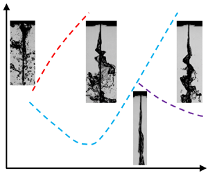
The change rule of the growth rate can be explained qualitatively. As shown in figure 19, the wavelength and the breakup length decreased with increasing  $W{e_g}$, indicating an enhancement of the instability. However, as shown in figure 19(a,b,e,f), the surface wave was regular when $W{e_g} < 0.3$, and the surface wave was in the axial direction rather than spanwise (i.e. the surface wave was approximately two-dimensional), so the two-dimensional model adopted in § 2.2 was also tenable. However, when $W{e_g} > 0.3$, as shown in figure 19(c,d,g,h), the surface wave was disordered. There were spanwise surface waves on the liquid sheet, so the growth rate obtained from the two-dimensional theoretical model inevitably resulted in some error. Additionally, due to the nonlinear effect, the disturbance could not increase infinitely, and a shorter wavelength corresponded to a lower saturated displacement. As a result, although the destabilizing and atomization phenomenon in figure 19(d) is more intense than that in figure 19(c), the difference in the disturbance displacement was not distinct due to the small wavelength. The measuring method for the growth rate was based on the disturbance displacement, and this method loses efficacy when the atomization is relatively intense. In conclusion, it was atomization intensity that determined whether the growth rate measuring method could be used. The method was critical when the surface wave was regular, but the growth rate can reflect the atomization intensity. According to figure 18, this method was able to measure the growth rate when $- {K_i} < 0.06$. Hereafter, for the condition of oscillating gas flow, $- {K_i} < 0.06$ was satisfactory to guarantee the correctness of the measuring results.

Figure 19. Destabilization of liquid sheet for different gas Weber numbers: (a)  $W{e_g} = 0.0927$; (b) $W{e_g} = 0.199$; (c) $W{e_g} = 0.453$; (d) $W{e_g} = 0.637$. Other parameters are same as figure 18. (e–h) Front views of (a–d), respectively: (e) $W{e_g} = 0.0927$; (f) $W{e_g} = 0.199$; (g) $W{e_g} = 0.453$; (h) $W{e_g} = 0.637$.
3.1.3. Growth rate in oscillating gas flow
In this section, experimental and theoretical growth rates are compared in the presence of oscillating gas flow. The theoretical results were obtained according to (2.8). Experiments were conducted using deionized water and glycerol aqueous solutions at different concentrations, and the corresponding physical parameters are listed in table 2. The viscosity differences versus various concentrations were the most obvious; the differences in density and surface tension were also non-negligible. Hence, the effect of a single physical factor was difficult to study. In the present work, the liquid velocity was adjusted to guarantee a constant liquid Weber number  $W{e_l}$.
Table 2. Physical parameters of water and glycerol aqueous solutions at different concentrations.

Due to the amplitude–frequency characteristics of the loudspeaker and the different acoustic field distributions at various frequencies in the tube, the relationship between the gas mean velocity and oscillation velocity also varied with oscillation frequency. Fitting the oscillating and mean velocity, the relationship was as follows:
 \begin{equation}\left. {\begin{array}{*{20}{c@{}}} {\Delta U = 1.809{U_{g,0}} - 2.500,\quad 100\ \textrm{Hz,}}\\ {\Delta U = 2.000{U_{g,0}} - 4.445,\quad 121\ \textrm{Hz,}}\\ {\Delta U = 1.903{U_{g,0}} - 3.944,\quad 142\ \textrm{Hz,}}\\ {\Delta U ={-} 0.1978U_{g,0}^2 + 4.31765{U_{g,0}} - 11.44,\quad 161\ \textrm{Hz,}}\\ {\Delta U ={-} 0.3654U_{g,0}^2 + 6.6875{U_{g,0}} - 19.99,\quad 177\ \textrm{Hz}\textrm{.}} \end{array}} \right\}\end{equation}
The curves of the non-dimensional growth rate  $- {K_i}$ versus increasing gas Weber number $W{e_g}$ were theoretically computed and compared with the experimentally measured values, as plotted in figure 20. It is important to remember that the frequency of the surface wave was equal to the gas oscillating frequency. Then, the growth rate corresponding to the oscillation frequency should be chosen as the theoretical growth rate. This is different from the condition of steady gas flow (figure 18), i.e. the theoretical growth rate may not be the maximum. This phenomenon can be explained physically: gas velocity oscillation inevitably modulates the surface wave in addition to providing an oscillating basic flow, so the disturbance with a frequency equal to the gas velocity oscillation frequency is much larger than other disturbances in the initial unstable stage. Therefore, this disturbance was observed in the image sequence.

Figure 20. Growth rate of solutions at different concentrations. (a) Deionized water:  ${U_l} = 1.820\ \textrm{m}\ {\textrm{s}^{ - 1}}$, $R{e_l} = 378.4$, $\rho \textrm{ = 0}\textrm{.0012}$, ${\varOmega _{s2}} = 0.0980$; (b) 20 % glycerol aqueous solution: ${U_l} = 1.779\ \textrm{m}\ {\textrm{s}^{ - 1}}$, $R{e_l} = 211.8$, $\rho = 0.00114$, ${\varOmega _{s2}} = 0.1005$; (c) 40 % glycerol aqueous solution: ${U_l} = 1.704\ \textrm{m}\ {\textrm{s}^{ - 1}}$, $R{e_l} = 93.7$, $\rho = 0.00109$, ${\varOmega _{s2}} = 0.1049$; (d) 60 % glycerol aqueous solution: ${U_l} = 1.635\ \textrm{m}\ {\textrm{s}^{ - 1}}$, $R{e_l} = 31.6$, $\rho = 0.00104$, ${\varOmega _{s\textrm{2}}} = 0.1093$. (Full line is theoretical curves; error bars are measured results; gas is air; ${\rho _g} = \textrm{1}\textrm{.2}\ \textrm{kg}\ {\textrm{m}^{ - \textrm{3}}}$, $a = 0.0002\ \textrm{m}$, ${f_s} = 142\ \textrm{Hz}$).
The effective gas Weber number  $W{e_{g2}} = {\rho _g}(U_{g,0}^2 + \Delta {U^2}/2)a/\sigma$ is defined to represent the aerodynamic force. This Weber number reflects the effect of the mean and oscillating gas velocity and has two advantages:
(1) In the K–H unstable region, destabilization of the surface wave was determined by the effective aerodynamic force, as stated in early work by the authors (Jia et al. Reference Jia, Xie, Yang, Fu and Cui2019, Reference Jia, Xie, Yang, Fu and Cui2020). This Weber number is considered the effective aerodynamic force.
(2) According to (3.2), the relationship between the mean and oscillating velocity changed with the frequency, so this Weber number could unify the mean and oscillating velocity, making comparison possible among the results of different frequencies.
The experimental and theoretical values in figure 20 coincide well, but the error bands were larger than those in figure 18. This is because the envelopes of the surface wave were spatially oscillatory, rather than a simple exponential growth, which may have introduced larger error bars. Although this reason affected the exact value, the measured growth rates were also important indicators to evaluate the instability. The experimental results showed that the growth rate increased with increasing concentrations of the solutions. In fact, the increasing concentration led to an increase in liquid density and viscosity, suppressing the instability; meanwhile, the increasing concentration induced a decrease in surface tension, enhancing the instability. In addition,  $W{e_l}$ was chosen as a constant, so the liquid velocity had to be reduced to guarantee the unchanged $W{e_l}$. As a result, the gas-to-liquid velocity increased, enhancing the instability. When the destabilizing factors predominated over the stabilizing factors, the growth rate increased. However, theoretical results showed that the growth rate barely changed with the concentration of the solutions. This may be because the present theory overestimated the stabilizing effect of liquid viscosity and liquid density.
Figure 21 displays the effect of  $W{e_l}$. The liquid velocity was changed to change $W{e_l}$, but the liquid Reynolds number and the non-dimensional frequency also changed. Therefore, the Ohnesorge number and the non-dimensional frequency were defined as $O{h_\textrm{l}} = {{\sqrt {W{e_l}} } / {R{e_l}}}$ and ${\varOmega _s} = {\omega _s}/\sqrt {\sigma /{\rho _\textrm{l}}{a^3}}$, respectively, which were independent of the liquid and gas velocities.

Figure 21. Effect of liquid Weber number on instability: (a)  $W{e_l} = 9.59$, (b) $W{e_l} = 10.63$, (c) $W{e_l} = 12.64$, (d) $W{e_l} = 14.98$ and (e) $W{e_l} = 17.29$. (Full lines are theoretical curves; error bars are measured results; liquid is deionized water; air is gas; ${\rho _g} = 1.2\ \textrm{kg}\ {\textrm{m}^{ - 3}}$, $a = 0.0002\ \textrm{m}$, ${f_s} = 142\ \textrm{Hz}$, $O{h_l} = 0.00819$, $\rho = 0.0012$, ${\varOmega _s} = 0.3037$.)
When the gas Weber number was relatively large, the growth rate decreased with increasing liquid Weber number. Theoretically, increasing the liquid Weber number should increase the liquid velocity (i.e. decreasing the gas-to-liquid velocity) and thus inhibit instability. According to Gaster (Reference Gaster1962), for a given temporal growth rate, the increase in group velocity leads to a decrease in the spatial growth rate, and the group velocity is almost directly proportional to the liquid velocity, i.e.
 \begin{equation}- \textrm{i}{k_i} \sim \frac{{{\beta _{tr}}}}{{{U_l}}}.\end{equation}
Therefore, the spatial growth rate decreased with increasing  $W{e_l}$. From another perspective, the increase in $W{e_l}$ indicated an increase in the liquid inertia force, which represents the ability of the liquid sheet to maintain its initial state. The higher inertia force made it more difficult to destabilize the liquid sheet. However, when $W{e_{g2}}$ was relatively small, the results were the opposite. A surface wave with a shorter wavelength is more difficult to motivate, and
 \begin{equation}\lambda \sim \frac{{{U_l}}}{{{\beta _i}}}.\end{equation}
 Obviously, the increase in liquid velocity led to an increase in the surface wavelength because the disturbance frequency was constant (equal to the oscillation frequency). Hence, the increase in  $W{e_l}$ led to an increased growth rate at small $W{e_{g2}}$.
Moreover, when  $W{e_{g2}}$ was relatively small, the measured growth rate was larger than the theoretical growth rate because the theoretical growth rate is a temporally mean growth rate in several periods. In fact, the liquid sheet was motivated by the gas pulse, inducing instantaneous growth, which was larger than the theoretically predicted mean growth rate. However, the experimental and theoretical results coincided well. Basically, the growth rate decreased with increasing $W{e_l}$ in the range studied.
The oscillating frequency of the gas velocity is also an important factor, as shown in figure 22. The liquid velocity was fixed in each panel to maintain  $W{e_l}$. The amplitude–frequency characteristic and the power of the loudspeaker were limited, and the form of the surface wave at a particular frequency was affected by the liquid velocity. The growth rates at oscillation frequencies of 100 and 121 Hz are shown in figure 22(a,c) and the growth rates at oscillation frequencies of 142, 161 and 177 Hz are shown in figure 22(b,d). Because the disturbance frequency and the liquid velocity significantly influenced the instability, the non-dimensional frequency ${\varOmega _{s2}} = {\omega _s}a/{U_l}$, used in figure 16, is also used here. When $W{e_{g2}}$ was relatively small (i.e. the aerodynamic force was relatively low), the low-frequency oscillation could induce larger wavelengths, and instability was more likely to be motivated; therefore, the growth rate of the low-frequency condition was higher than that of the high-frequency condition. However, with an increase in the aerodynamic force, the surface wave could also be motivated under high-frequency conditions. The growth rate increased quickly with increasing $W{e_{g2}}$, even tending to exceed the low-frequency condition. This was determined by the dispersion relation of the instability. When $W{e_{\textrm{g}2}}$ was larger, the high-frequency surface wave could be closer to the dominant frequency (the frequency corresponding to the maximum growth rate), so the growth rate could be faster.

Figure 22. Effects of oscillation frequency on growth rate: (a,c)  ${U_l} = 1.56\ \textrm{m}\ {\textrm{s}^{ - 1}}$, $W{e_l} = 7.01$; (b,d) ${U_l} = 2.07\ \textrm{m}\ {\textrm{s}^{ - 1}}$, $W{e_l} = 12.41$. (Full lines are theoretical curves; error bars are measured results; liquid is deionized water; air is gas; ${\rho _g} = 1.2\ \textrm{kg}\ {\textrm{m}^{ - 3}}$, $a = 0.0002\ \textrm{m}$, $O{h_l} = 0.00819$, $\rho = 0.0012$.)
Furthermore, the gas-to-liquid relative velocity was an important parameter to evaluate the driving force of instability, so the relative Weber number was defined as  $W{e_{rel}} = {\rho _g}[{({U_l} - {U_{g,0}})^2} + \Delta {U^2}/2]a/\sigma $, which can reflect the driving force of instability more accurately than $W{e_{g2}}$. Relative Weber number $W{e_{rel}}$ was set as the x coordinate, as shown in figure 22. The general rule of the growth rates in figure 22(c,d) is the same as in figure 22(a,b): a larger $W{e_{rel}}$ was needed to motivate the instability of a high-frequency disturbance.
3.2. Patterns of surface wave
Section 3.1 discusses the growth rate of the surface wave. In fact, the conditions discussed in § 3.1 involved only one form of surface wave: the surface wave with a frequency equal to the gas velocity oscillation. In this section, a larger parameter range is considered, four unstable modes of the surface wave are found according to the experimental study and linear instability theory discussed in § 2.2 is used to divide the distribution of these different wave patterns.
3.2.1. Distribution of different patterns of surface waves
Figure 23 shows the distribution of the patterns of the surface wave in the parameter range considered in the present study. The frequency of the surface wave was obtained using POD, and the frequency of the first two dominant modes was regarded as the dominant frequency of the surface wave. When the oscillating frequency was moderate and  $W{e_{rel}}$ was large (i.e. region 1 marked in figure 23), the frequency of the surface wave was half the oscillating frequency. In this region, the non-dimensional oscillating frequency ${\varOmega _{s2}}$ was relatively high, corresponding to a short disturbance wavelength, but the aerodynamic force was not high enough to motivate the disturbance. As a result, a longer wave pattern was selected by the unstable system, and due to the forcing effect of gas oscillation, half the frequency of gas oscillation was selected. This surface wave pattern was defined as the K–H subharmonic mode (KHS), shown in figure 24(a).

Figure 23. Distribution of different forms of surface waves in parameter space. 1, KHS; 2, KHH; 3, FDM; 4, SDM. (Liquid is deionized water; air is gas;  ${\varOmega _w} = \omega a/{U_l}$ is non-dimensional frequency of surface wave; ${\rho _g} = 1.2\ \textrm{kg}\ {\textrm{m}^{ - 3}}$, $a = 0.0002\ \textrm{m}$, ${f_s} = 177\ \textrm{Hz}$, $O{h_l} = 0.00819$, $\rho = 0.0012$.)

Figure 24. Various patterns of surface wave. (a) KHS:  ${U_l} = 1.94\ \textrm{m}\ {\textrm{s}^{ - 1}}$, ${U_{g,0}} = 7.25\ \textrm{m}\ {\textrm{s}^{ - 1}}$, $\Delta U = 9.28\ \textrm{m}\ {\textrm{s}^{ - 1}}$, $W{e_{rel}} = 0.248$, ${\varOmega _{s2}} = 0.1144$; (b) KHH: ${U_l} = 2.26\ \textrm{m}\ {\textrm{s}^{ - 1}}$, ${U_{g,0}} = 7.22\ \textrm{m}\ {\textrm{s}^{ - 1}}$, $\Delta U = 9.25\ \textrm{m}\ {\textrm{s}^{ - 1}}$, $W{e_{rel}} = 0.235$, ${\varOmega _{s2}} = 0.0986$; (c) FDM: ${U_l} = 1.65\ \textrm{m}\ {\textrm{s}^{ - 1}}$, ${U_{g,0}} = 5.39\ \textrm{m}\ {\textrm{s}^{ - 1}}$, $\Delta U = 5.47\ \textrm{m}\ {\textrm{s}^{ - 1}}$, $W{e_{rel}} = 0.101$, ${\varOmega _{s2}} = 0.1351$; (d) SDM: ${U_l} = 1.58\ \textrm{m}\ {\textrm{s}^{ - 1}}$, ${U_{g,0}} = 6.38\ \textrm{m}\ {\textrm{s}^{ - 1}}$, $\Delta U = 7.80\ \textrm{m}\ {\textrm{s}^{ - 1}}$, $W{e_{rel}} = 0.186$, ${\varOmega _{s2}} = 0.1407$. (Liquid is deionized water; air is gas; ${\rho _g} = 1.2\ \textrm{kg}\ {\textrm{m}^{ - 3}}$, $a = 0.0002\ \textrm{m}$, ${f_s} = 177\ \textrm{Hz}$, $O{h_l} = 0.00819$, $\rho = 0.0012$.)
When  $W{e_{rel}}$ was proportionately large and the non-dimensional oscillating frequency was low (i.e. region 2 marked in figure 23), the frequency of the surface wave equalled the oscillating frequency. The wave pattern is shown in figure 24(b). This wave pattern was of a regular form, which is used in § 3.1 to investigate the growth rate. Hereafter, this pattern is referred to as the K–H harmonic mode (KHH).
When  $W{e_{rel}}$ was relatively small (i.e. region 3 marked in figure 23), the frequency of the surface wave was independent of the oscillating frequency because the aerodynamic force was too small to motivate the surface wave of the KHS and KHH. As shown in figure 24(c), the wave was disordered, referred to as the first disordered mode (FDM).
When  $W{e_{rel}}$ and the non-dimensional oscillating frequency were both relatively large (region 4 in figure 23), the non-dimensional oscillating frequency was inversely proportional to the liquid velocity, and $W{e_{rel}}$ represented the aerodynamic force. Thus, due to the increased ratio of momentum between gas and liquid, in this condition, the breakup time of the liquid sheet was shorter than one period. The oscillating growth of the surface wave did not occur in this condition, as shown in figure 24(d). This pattern exceeded the scope of the theoretical results in § 2.2; this pattern is referred to as the second disordered mode (SDM).
The four different unstable modes discovered in the experimental study are shown in supplementary movies 4–7.
Figure 23 also shows an apparent boundary between the KHH and KHS. These two patterns were sensitive to the non-dimensional oscillating frequency. Due to the competition between the two modes, the surface wave was not regular near the boundary. In addition, the boundary between KHH and FDM and the boundary between KHS and SDM were not apparent. There were some KHH and KHS in the SDM region, indicating that the wave pattern was not sensitive to  $W{e_{rel}}$ and that the range of $W{e_{rel}}$ near the boundary was relatively large. Moreover, the boundary between KHS and FDM was not monotonic. With an increase in non-dimensional frequency, $W{e_{rel}}$ near the boundary decreased and then increased. With an increase in non-dimensional frequency, the liquid velocity decreased, and the range of unstable disturbance frequency narrowed, so the surface wave with a certain frequency was more difficult to motivate. With an increase in the non-dimensional oscillating frequency (namely a decrease in the liquid velocity), the ratio of momentum between gas and liquid decreased, restraining the instability. The effects of these two factors were opposite, and competition made the boundary non-monotonic. There was also a distinct boundary between the KHS and SDM. The increase in non-dimensional frequency indicated an increased ratio of momentum between gas and liquid; thus, a lower $W{e_{rel}}$ could motivate a surface wave of SDMs. Therefore, the critical $W{e_{rel}}$ corresponding to the boundary was a monotonic decreasing function of oscillating frequency.
To theoretically explain the patterns of surface waves shown in figure 23,  $W{e_l}$ was adopted as the x coordinate to map the distribution again in figure 25. The surface tension was constant, so $W{e_l}$ represents the inertia force of the liquid sheet; $W{e_{rel}}$ represents the coupling effect of the aerodynamic and oscillating forces (i.e. the effective aerodynamic force) and, therefore, the relative scale of these two forces can be obtained visually. As previously noted, SDM was caused by the breakup of the liquid sheet within a time frame smaller than an oscillating period; the instability was strong. Hence, the growth rate at the boundary between SDM and KHS must reach a critical value. This boundary is defined as 1–4, as shown in figure 25. The upper left region of this line is the SDM region. In terms of frequency, most points in the SDM region are subharmonic rather than irregular. However, this does not prove that the pattern of the surface wave was also regular. As shown in figure 27(a), there was not an entire wavelength, although the disturbance frequency was half the oscillating frequency of the gas flow. The atomization was so strong that the ruptured liquid sheet obstructed the gas nozzle exit, influencing the amplitude of gas oscillation. At small $W{e_l}$, $W{e_{rel}}$ could not be greatly improved in the SDM region, although the power of the loudspeaker was turned up. This was also the reason why the points were so dense in the SDM region. Generally, patterns such as those in figure 27(a) are regarded as SDM.

Figure 25. Theoretical boundary between different patterns. 1, KHS; 2, KHH; 3, FDM; 4, SDM. (Liquid is deionized water; air is gas;  ${\rho _g} = 1.2\ \textrm{kg}\ {\textrm{m}^{ - 3}}$, $a = 0.0002\ \textrm{m}$, ${f_s} = 177\ \textrm{Hz}$, $O{h_l} = 0.00819$, $\rho = 0.0012$, ${\varOmega _s} = 0.3786$.)
Figure 26 is plotted to explain the locations of boundaries 1–3-a and 2–3. The dispersion curves of a, b and c and d, e and f shown in figure 25 are plotted in figures 26(a) and 26(b), respectively. Boundaries 1–3-a and 1–3-b are the lower boundaries of the KHS, which separates the KHS from the FDM and KHH. The evaluation criterion of 1–3-a is
 \begin{equation}- {K_{i,sub}} ={-} {A_1}{K_{i,max}},\end{equation}
where  $- {K_{i,sub}}$ and $- {K_{i,max}}$ are the growth rates corresponding to half the frequency of gas oscillation and the maximum growth rate, respectively, as shown in figure 26(a). Factor ${A_\textrm{1}}$ is a correction factor, set as $\textrm{0}\textrm{.96}$ in figure 25. In the KHS region, the aerodynamic effect was relatively high, satisfying $- {K_{i,sub}} > - {A_1}{K_{i,max}}$, so the surface wave pattern was subharmonic. According to the theoretical results in § 2.2, a longer surface wave corresponded to a lower critical aerodynamic force, and the improvement of $W{e_l}$ led to the increased wavelength at a specific frequency. Hence, $W{e_{rel}}$ corresponding to 1–3-a decreased with increasing $W{e_\textrm{l}}$. However, with increased liquid velocity, the liquid inertia force increased; as a result, the growth rate decreased with a given aerodynamic force – the liquid sheet was more difficult to disturb. Consequently, a larger aerodynamic force was needed to motivate the instability. Here, the relationship is $W{e_{rel}} = {A_2}W{e_l} = 0.018W{e_l}$, and 1–3-b can then be obtained, which divides the KHS and KHH regions well. Note that there were some KHH conditions in the KHS region around point $W{e_{rel}} = 0.24,\ W{e_l} = 12$; these are explained in figure 28.


Figure 27. Two typical conditions in figure 25. (a) Typical atomization phenomenon in SDM region, where frequency of surface wave is half the oscillating frequency ( $W{e_l} = 4.898$, $W{e_{rel}} = 0.231$). (b) Typical atomization phenomenon in FDM region where frequency of surface wave equals the oscillating frequency ( $W{e_l} = 14.128$, $W{e_{rel}} = 0.089$).

Figure 28. Pattern distribution of surface waves at different frequencies. 1, KHS; 2, KHH; 3, FDM: (a)  ${A_2} = 0.0202$, ${A_3} = 0.0001$, $W{e_{l,cr}} = 4.95$, ${U_{g,2}} = 1.14{U_g}$, ${f_s} = 100\ \textrm{Hz}$, ${\varOmega _s} = 0.2139$; (b) ${A_2} = 0.018$, ${A_3} = 0.0001$, $W{e_{l,cr}} = 6.35$, ${f_s} = 121\ \textrm{Hz}$, ${\varOmega _s} = 0.2558$; (c) ${A_2} = 0.016$, ${A_3} = 0.5$, ${A_4} = 0.96$, $W{e_{l,cr}} = 8.75$, ${f_s} = 142\ \textrm{Hz}$, ${\varOmega _s} = 0.3037$; (d) ${A_2} = 0.018$, ${A_3} = 0.93$, ${A_4} = 0.98$, $W{e_{l,cr}} = 8.9$, ${f_s} = 161\ \textrm{Hz}$, ${\varOmega _s} = 0.3444$. (Liquid is deionized water; air is gas; other parameters are the same as figure 25.)
Using a method similar to that for 1–3-a, the evaluation criterion of 2–3 is
 \begin{equation}- {K_{i,h}} ={-} {A_3}{K_{i,max}},\end{equation}
where  $- {K_{i,h}}$ and $- {K_{i,max}}$ are the growth rates corresponding to the frequency of gas oscillation and the maximum growth rate, respectively, as shown in figure 26(b). Factor ${A_\textrm{3}}$ is a correction factor, set as $\textrm{0}\textrm{.82}$ in figure 25. The regions above and below this boundary are the KHH and FDM regions, respectively. Several points in the FDM region can be found with a harmonic frequency. However, a typical image of these points shown in figure 27(b) proved that the disturbance displacement was small, and there was no regular wavelength, so these points were also regarded as FDM.
3.2.2. Influence of oscillation frequency
Figure 28 displays the pattern distribution at different gas velocity oscillations. With an increase in oscillation frequency,  $W{e_l}$ corresponding to the boundary between the KHS and KHH regions increased. When $W{e_{rel}}$ was given, a larger liquid velocity was needed to involve the oscillation frequency into the unstable frequency region with a larger oscillation frequency, so the corresponding $W{e_l}$ increased. Note that this boundary was more complex than that in figure 25. For example, in figure 28(d), 1–3-b still agrees with the relation $W{e_{rel}} = 0.018W{e_l}$. However, 1–3-b cannot divide the KHH and KHS regions completely, so another mechanism was considered to divide these two regions. According to the criterion of 2–3, the occurrence of KHH requires the growth rate to reach a critical value, i.e. $- {K_{i,h}} > - {A_3}{K_{i,max}}$. Likewise, boundary 1–2-b can be obtained according to a similar criterion $- {K_{i,h}} ={-} {A_4}{K_{i,max}}$, where ${A_4} = 0.98$ in figure 28(d). Moreover, with an increase in $W{e_{rel}}$, the boundary between KHH and KHS corresponds to a critical liquid Weber number $W{e_{l,cr}}$, which is boundary 1–2-a. Furthermore, with an increase in the oscillation frequency, boundary 1–2-b became more important, as shown in figure 28(c,d), whereas boundary 1–2-b could not be observed when the oscillation frequency was relatively low, as shown in figure 28(a,b).
In figure 29, the non-dimensional frequency  ${\varOmega_{s\textrm{2}}}$ is set as the x coordinate to further study the effect of frequency. The ratio between $W{e_{rel}}$ and $W{e_l}$ is set as the y coordinate. The boundaries in figures 25 and 28 are marked in figure 29. The relationship between the boundaries and frequency is more specific in figure 29. According to the pattern distribution, the critical frequencies ${\varOmega _{scr1}}$ and ${\varOmega _{scr2}}$ between the KHH and KHS regions are shown in table 3. For a relatively large $W{e_{rel}}/W{e_l}$, when ${\varOmega _{s2}} < {\varOmega _{scr1}}$, the pattern was KHH; when ${\varOmega _{s2}} > {\varOmega _{scr2}}$, the pattern was KHS; and ${\varOmega _{scr1}} < {\varOmega _{s2}} < {\varOmega _{scr2}}$ was a competitive range between the two modes. As shown in table 3, the critical frequencies were located in the range 0.0962–0.1193 with a relative change range of 24 %. The range of the oscillating frequency was 100–177 Hz with a relative change range of 77 %. Recall that the non-dimensional frequency was ${\varOmega _{s2}} = {\omega _s}a/{U_l}$, which can be regarded as the ratio between the gas oscillating frequency and the physically inherent frequency. The physical process of the instability can be explained qualitatively: when the dimensional frequency ${\omega _s}$ increased, the wavelength was approximately inversely proportional to the gas oscillating frequency $\lambda \sim {U_l}/{\omega _s}$. Instability was more difficult to motivate for a shorter wavelength; therefore, when the oscillating frequency ${\omega _s}$ increased and the aerodynamic force remained unchanged, motivation of the KHH and KHS required an increase in the wavelength (i.e. an increase in ${U_l}$). As a result, the numerator and denominator both increased in the expression of non-dimensional frequency ${\varOmega _{s2}} = {\omega _s}a/{U_l}$. Therefore, the range of critical frequencies did not change notably, especially for ${\varOmega _{scr1}}$, the range of change was 0.0962–0.1051 and the relative change range was smaller than 10 %. To summarize, if the KHH or KHS must be maintained, then the liquid velocity should be adjusted to maintain ${\varOmega _{s2}}$ when the gas oscillating frequency changes.

Figure 29. Pattern distribution when non-dimensional frequency is set as x coordinate. 1, KHS; 2, KHH; 3, FDM; 4, SDM: (a)  ${f_s} = 100\ \textrm{Hz}$, ${\varOmega _s} = 0.2139$; (b) ${f_s} = 121\ \textrm{Hz}$, ${\varOmega _s} = 0.2558$; (c) ${f_s} = 142\ \textrm{Hz}$, ${\varOmega _s} = 0.3037$; (d) ${f_s} = 161\ \textrm{Hz}$, ${\varOmega _s} = 0.3444$; (e) ${f_s} = 177\ \textrm{Hz}$, ${\varOmega _s} = 0.3786$. (Liquid is deionized water; air is gas; other parameters are the same as figure 25.)
Table 3. Critical frequencies between KHH and KHS regions.

Moreover, it can be seen that no boundary 1–2-b existed when the oscillating frequency was low, possibly because when the oscillating frequency was small – and if a frequency of surface wave had to be restricted within a small range – the liquid velocity range requiring adjustment was small, which exceeds the accuracy limitations of the equipment. Generally, when  $W{e_{rel}}/W{e_l}$ was small, the pattern was FDM; when $W{e_{rel}}/W{e_l}$ was moderate and the non-dimensional frequency was relatively high, the pattern was KHS; and when $W{e_{rel}}/W{e_l}$ was moderate and the non-dimensional frequency was relatively small, the pattern was KHH. When both $W{e_{rel}}/W{e_l}$ and the non-dimensional frequency were relatively large, the pattern was SDM.
Considering figures 25 and 29 together, at boundary 1–3-b,  $W{e_{rel}}/W{e_l}$ is approximately 0.018, and the relative error is smaller than 12 %. However, at low frequencies, $W{e_l}$ was relatively small, and the spatial damping was also small. Hence, in figure 28(a,b), boundary 2–3 corresponds to the condition when the growth rate was slightly larger than one. In addition, a correction was conducted for the condition of figure 28(a). In the process of dealing with the gas velocity, the aerodynamic force was underestimated. As shown in figure 10, the FFT process reduced the effective value of the aerodynamic force. Therefore, ${U_{g,2}} = 1.14{U_g}$ was adopted to correct the gas velocity, and boundary 2–3 could be obtained. With increasing frequency, $W{e_l}$ corresponding to 2–3 increases, leading to an increase in the corresponding $W{e_{rel}}$. As a result, ${A_\textrm{3}}$ increased. In other words, motivation for the KHH requires a higher liquid velocity at a higher frequency, so a greater aerodynamic force is needed to overcome the liquid inertia force.
Comparing figures 28(c) and 28(d), with increasing frequency, the minimum  $W{e_{rel}}$ on boundary 1–2-b also increases, consistent with the rule that ${A_\textrm{2}}$ changes little with frequency. In figure 28(d), the minimum $W{e_{rel}}$ on 1–2-b was approximately 0.21. Therefore, at a higher oscillating frequency (shown in figure 25), the power of the loudspeaker was not high enough to observe 1–2-b. However, in the description of figure 25, there are some KHH conditions in the KHS region around point $W{e_{rel}} = 0.24,\ W{e_l} = 12$. According to 1–2-b in figures 28(c) and 28(d), these points were not accidental errors but part of the KHH region above 1–2-b.
The frequency of the surface wave in the FDM region was investigated. As shown in figure 30, the theoretical frequencies corresponding to the maximum growth rate were obtained, and the experimental frequencies of the dominant modes of POD are also displayed. With an increase in  $W{e_{rel}}$, the experimental and theoretical frequencies both increased with an increase in $W{e_{rel}}$. The reason is that the increase in $W{e_{rel}}$ indicates an increasing aerodynamic force, broadening the unstable frequency range and promoting the dominant unstable frequency.

Figure 30. Frequencies corresponding to maximum growth rates of surface waves in FDM region shown in figure 28(c).
Furthermore, in the low-frequency condition in figure 28(a,b), the surface waves with irregular frequencies were fewer than in the high-frequency condition. Although these points were separated into the FDM region, the frequency of the surface wave equalled the gas oscillating frequency. This phenomenon is worthy of further study. Figure 31 displays the surface wave frame by frame to investigate the waveform. Here POD was also conducted to analyse the waveform.

Figure 31. (a–u) Typical waveform in FDM region shown in figure 28(a) ( $W{e_l} = 5.421$, $W{e_{rel}} = 0.0673$).
The frame rate of figure 31 is 2000 fps, and the gas oscillating frequency is 100 Hz. Twenty images constitute an oscillating period; therefore, 21 continuous images are displayed. The phase and forms of the wave in figure 31(u) were nearly the same as those in figure 31(a); the periodicity of the surface wave was good, and the wave frequency was equal to the gas oscillating frequency. However, this cannot demonstrate that the wavelength is equal to the ratio between the wave velocity and frequency. Instead, by selecting a wave crest as a reference point and following this point frame by frame, an interesting phenomenon is revealed: after a period, the crest transforms into a trough, which is not a typical travelling wave but – like a standing wave – spreads spatially, i.e. a travelling Faraday wave. According to figure 31, the travelling distance of the surface wave in one period was just 1.5 times that of the wavelength.
This pattern was not observed in the high-frequency condition, possibly because under those conditions, there was more spatial dissipation of oscillating amplitude, which was not intense enough to motivate the Faraday wave.
The qualitative description of this pattern can be expressed as
 \begin{equation}\eta = {\eta _0}\cos (\omega t + kx)\cos ({\omega _s}t/2),\end{equation}
where  ${\omega _s}$ is the oscillating frequency. Here ${\omega _s}/2$ was chosen because the oscillating frequency of the surface wave was half the gas oscillating frequency. (The crest became a trough, indicating half the period of the oscillation of the surface wave.) Frequency $\omega $ is the travelling frequency. In a gas oscillating period, the surface wave travelled 3/2 times that of the wavelength, so $\omega = 3{\omega _s}/2$. Therefore, (3.7) becomes
 \begin{equation}\begin{aligned} \eta & = {\eta _0}\cos (3{\omega _s}t/2 + kx)\cos ({\omega _s}t/2)\\ & = {\eta _{02}}\cos (2{\omega _s}t + kx) + {\eta _{02}}\cos ({\omega _s}t + kx),\ {\eta _{02}} = {\eta _0}/2. \end{aligned}\end{equation}
 According to (3.8), the surface wave can be decomposed into two sets of modes with frequencies of  ${\omega _s}$ and $\textrm{2}{\omega _s}$. The wavelengths of these two modes were the same; therefore, wavelength is a reliable criterion. Double-frequency modes rising in a standard travelling wave are often induced by the nonlinear effect, and their wavelength is half – rather than equal to – that of the linear modes.
Figure 32 is the POD result of the surface wave in figure 31. Modes 1–4 were all antisymmetric, dominating the waveform. The energy ratio of modes 1–4 exceeded 50 %, indicating that the waveform was fairly regular. Modes 1 and 2 constituted a set with a frequency of 100 Hz, while modes 3 and 4 constituted a set with a frequency of 200 Hz. These results coincided well with the prediction in (3.8). There was not a significant difference between the wavelengths of modes 1 and 2 and the wavelengths of modes 3 and 4, indicating that modes 3 and 4 were not nonlinear harmonic waves but were induced by  ${\eta _{02}}\cos (2{\omega _s}t + kx)$ in (3.8). Therefore, the POD results also proved that the surface wave in figure 31 was a standing wave, spreading spatially, namely a travelling Faraday wave. These results confirmed that when the oscillating frequency and $W{e_{rel}}$ were relatively low and $W{e_l}$ was relatively high, parametric instability could be motivated. Under this condition, the waveform cannot be regarded as a disordered wave, i.e. boundary 2–3 in figure 28 can guarantee that the points above it are K–H harmonic waves but cannot guarantee that the points below it are all disordered waves. A Faraday wave may also be motivated in the FDM region. However, note that the conditions for the motivation of Faraday waves are rigorous, requiring a low spatial dissipation of gas oscillations. Meanwhile, it was difficult for the growth rate in the parametric unstable region to surpass the K–H unstable region if the mean relative velocity between the gas and liquid was relatively high. Therefore, only a few Faraday wave points were observed. Although the repeatability of these points was good, the points were not sufficient to separate into a specific region.

Figure 32. The POD results shown in figure 31. (a) Energy distribution, (b) frequency of modes 1–4, (c) mode 1, (d) mode 2, (e) mode 3 and (f) mode 4.
Moreover, the schematics of this mode are presented in supplementary movies 8 and 9.
3.2.3. Influence of solution concentration
Figure 33 displays the pattern distribution using a liquid solution with a different concentration. An increase in the mass fraction of glycerol led to increased density and viscosity, which restrained the instability. At the same time, an increase in the mass fraction of glycerol led to a decrease in the surface tension, enhancing the instability. As shown in figure 33, with increasing concentration, the coefficients  ${A_\textrm{2}}$ and ${A_\textrm{3}}$ tended to increase. Coefficients ${A_\textrm{2}}$ and ${A_\textrm{3}}$ corresponded to the criteria of 1–3-b and 2–3, respectively. Hence, an increase in these two coefficients indicated that KHH and KHS motivation required greater aerodynamic force.

Figure 33. Effects of solution concentration on pattern distribution. 1, KHS; 2, KHH; 3, FDM. Liquid: (a) deionized water;  ${A_2} = 0.016$, ${A_3} = 0.5$, ${A_4} = 0.96$, $W{e_{lcr}} = 8.75$, $O{h_l} = \textrm{0}\textrm{.00819}$, $\rho = 0.0012$; (b) 20 % glycerol aqueous solution; ${A_2} = 0.0175$, ${A_3} = 0.8$, ${A_4} = 0.95$, $W{e_{lcr}} = 8.45$, $O{h_l} = 0.0147$, $\rho = 0.00114$; (c) 20 % glycerol aqueous solution; ${A_2} = 0.0195$, ${A_3} = 0.8$, ${A_4} = 0.965$, $W{e_{lcr}} = 8.5$, $O{h_l} = 0.0329$, $\rho = 0.00109$; (d) 60 % glycerol aqueous solution; ${A_2} = 0.0235$, ${A_3} = 0.85$, $W{e_{lcr}} = 9.2$, $O{h_l} = 0.0974$, $\rho = 0.00104$. Gas: air ( $\,{f_s} = 142\ \textrm{Hz}$, ${\varOmega _{s2}} = 0.3037$).
Note that the x coordinate was set as  $W{e_l}$, which included the effect of liquid density and surface tension, so liquid viscosity was the main parameter affecting the instability. However, in earlier studies by the authors (Yang et al. Reference Yang, Jia, Fu and Yang2018; Jia et al. Reference Jia, Xie, Yang, Fu and Cui2019), the viscosity did not dramatically affect the growth rate. This may be because these studies – including the present theoretical study – did not consider the velocity distribution in the basic liquid flow. When the aerodynamic force was relatively low, the liquid velocity distribution could increase the dissipation effect, restraining instability. However, when the aerodynamic force was relatively high (as shown in figure 20), the restraining effect of viscosity was not distinct. In general, viscosity mainly promoted the aerodynamic force required for motivating KHS and KHH, but it had little effect on instability at a relatively high aerodynamic force.
4. Conclusion
An experimental study of the oscillatory K–H instability of a planar liquid sheet in the presence of axial oscillating gas flow was conducted. The growth rates of the surface waves were measured for both steady and oscillatory gas flow cases and compared with theoretical predictions using linear instability theory. The experimentally measured growth rates were compared with those obtained using linear instability theory. Moreover, in a larger parameter range, four typical wave modes were found through experimental study. The mechanism of the occurrence of these modes was analysed physically. Based on a physical interpretation of these modes, linear instability theory was used to divide the boundaries between the regimes of these modes, and the theoretical boundaries can divide these regimes well with appropriate correction factors.
Examination of the growth rate demonstrated two effects of gas oscillation: modulating the surface wave and providing an oscillating aerodynamic force. An increase in the gas oscillating frequency suppressed instability when the aerodynamic force was low, but it had little influence on the growth rate when the aerodynamic force was high. Increasing the liquid inertia force mainly restrained instability. Liquid viscosity had little influence on the instability when the aerodynamic force was relatively high. However, an increase in liquid viscosity had a dramatic stabilizing effect. The experimental results agreed well with the theoretical results.
In a larger parameter range, an interesting experimental discovery was finding four different unstable wave patterns: FDM, SDM, KHH and KHS. The frequencies of KHH and KHS equalled the gas oscillating frequency and half the gas oscillating frequency, respectively; the frequencies of FDM and SDM were disordered. All of these modes primarily corresponded to the K–H instability rather than the parametric instability. The KHS was an unexpected but surprising phenomenon. It did not belong to the parametric unstable region, but its frequency was half the forcing frequency. According to linear theory, a disturbance with a longer wavelength is more likely to be motivated. For a certain liquid Weber number, the wavelength of KHS was longer than that of KHH, and the subharmonic oscillations of KHS could also couple with the oscillating gas flow. As a result, KHS occurred in the present study. The FDM was located in the region where the relative Weber number was small. If the liquid Weber number was relatively small, then with an increase in aerodynamic force, the dominant frequency in FDM increased until it reached the frequency of KHS. However, if the liquid Weber number was relatively large, then an increase in aerodynamic force made the unstable mode transform from FDM to KHH. From the KHS region, if the aerodynamic force increased until the liquid sheet broke up within one period, then the unstable mode transformed from KHS to SDM. If the gas oscillating frequency increased, then a larger aerodynamic and liquid inertia force was required to maintain KHH, while the boundary between KHS and FDM remained almost unchanged. With an increase in viscosity, the minimum aerodynamic force for the motivation of KHH and KHS increased, indicating that the viscous dissipation effect is more significant at lower gas Weber numbers.
Another interesting phenomenon was the discovery of the travelling Faraday wave when the liquid inertia force was high and the aerodynamic force was low. The oscillating and travelling frequencies were half the gas oscillating frequency and 3/2 times the gas oscillating frequency, respectively.
Supplementary movies
Supplementary movies are available at https://doi.org/10.1017/jfm.2023.19.
Funding
This research was supported by Fundamental Research Funds for the Central Universities (no. 2022JBMC035), Youth Science Fund Project of National Natural Science Foundation of China (no. 12102358), Fundamental Research Funds for the Central Universities (no. 3102021HHZY030008), China Postdoctoral Science Foundation (no. 2020M692617), Natural Science Foundation of Chongqing of China (cstc2021jcyj-msxmX0393) and Young Talent Fund of Association for Science and Technology in Shaanxi, China.
Declaration of interests
The authors report no conflict of interest.
Appendix A
According to Jia et al. (Reference Jia, Xie, Yang, Fu and Cui2019), the temporal stability of viscoelastic planar liquid sheets in the presence of gas oscillations can be solved using Floquet theory. In the present study, the liquid sheet was viscous; therefore, the dispersion relation of temporal stability could be obtained by simplifying the constitutive equation of the liquid sheet. As shown in figure 34, the liquid sheet was two-dimensional with a thickness of 2a. The basic flows of the gas medium and liquid phase were oscillating and static, respectively. The disturbance amplitude of the surface wave was  $\eta $. The x and y axes were parallel and perpendicular to the stream of the gas flow.

Figure 34. Temporal instability of planar liquid sheet under (a) sinuous and (b) varicose disturbance.
Actually, in the reference system where the nozzle is static, the liquid sheet is oscillatory because of the oscillation of the gas velocity. The liquid and gas velocities can be expressed as
 \begin{gather}{U_l} = {U_{l,0}} + \mathrm{\Delta }{U_l}f(t),\end{gather}
 \begin{gather}{U_{g1}} = {U_{g,0}} + \mathrm{\Delta }{U_g}\cos ({\omega _s}t).\end{gather}
For the basic flow, the liquid velocity is independent of spatial coordinate, so the liquid viscous stress is zero. So according to Kelly (Reference Kelly1965), the liquid and gas velocity satisfies
 \begin{equation}\frac{{\textrm{d}{U_l}/\textrm{d}t}}{{\textrm{d}{U_{g1}}/\textrm{d}t}} = \frac{{{\rho _g}}}{{{\rho _l}}}.\end{equation}
Therefore, the liquid velocity is
 \begin{equation}{U_l} = {U_{l,0}} + \frac{{{\rho _g}}}{{{\rho _l}}}\mathrm{\Delta }{U_g}\cos ({\omega _s}t).\end{equation}
However, it should be noted that  $\mathrm{\Delta }{U_l}$ is much smaller than the gas velocity oscillation. Therefore, in the stability analysis in § 2.2, the liquid velocity oscillation is ignored, which has little effect on the growth rate of the surface wave.
In the present study, the reference system is selected such that the liquid sheet is static. Therefore, the governing equations of the liquid phase are the conservation laws of mass and momentum, as follows:
 \begin{gather}\boldsymbol{\nabla }\boldsymbol{\cdot }{\boldsymbol{v}_{\boldsymbol{l}}} = 0,\end{gather}
 \begin{gather}{\rho _\textrm{l}}\left( {\frac{\partial }{{\partial t}} + {\boldsymbol{v}_{\boldsymbol{l}}}\boldsymbol{\cdot }\boldsymbol{\nabla }} \right){\boldsymbol{v}_{\boldsymbol{l}}} = {\rho _\textrm{l}}\boldsymbol{g} - \boldsymbol{\nabla }{p_\textrm{l}} + \mu {\nabla ^2}{\boldsymbol{v}_{\boldsymbol{l}}},\end{gather}
where  ${\rho _l}$ is the liquid density, t is time, ${\boldsymbol{v}_{\boldsymbol{l}}}$ is the liquid velocity vector (expressed as $({u_\textrm{l}},{v_\textrm{l}})$), ${p_l}$ is liquid pressure and $\mu $ is viscosity of the liquid phase. It should be noted that the reference system is a non-inertial system, so there exists an inertia body force ${\rho _l}g$ in (A6), where $\boldsymbol{g} = (g,0)$ and $g ={-} \textrm{d}{U_l}/\textrm{d}t = ({\rho _g}/{\rho _l}){\omega _s}\mathrm{\Delta }{U_g}\sin ({\omega _s}t)$.
The governing equations of the incompressible inviscid medium can be expressed as
 \begin{gather}\boldsymbol{\nabla }\boldsymbol{\cdot }{\boldsymbol{v}_{\boldsymbol{g}}} = 0,\end{gather}
 \begin{gather}{\rho _g}\left( {\frac{\partial }{{\partial t}} + {\boldsymbol{v}_{\boldsymbol{g}}}\boldsymbol{\cdot }\boldsymbol{\nabla }} \right){\boldsymbol{v}_{\boldsymbol{g}}} = {\rho _g}\boldsymbol{g} - \boldsymbol{\nabla }{p_g},\end{gather}
where  ${\rho _g}$ is the gas density, ${\boldsymbol{v}_{\boldsymbol{g}}}$ is the gas velocity vector, which can be expressed as $({u_{g,}}{v_g})$, and ${p_g}$ is the gas pressure.
When the disturbance began, the upper and lower interfaces were displaced and regarded as one of the following forms:
 \begin{equation}\left. {\begin{array}{*{20}{c@{}}} {{Y_j} = {{( - 1)}^j}a + \eta (x,t),\ \textrm{for}\ \textrm{sinuous}\ \textrm{mode,}}\\ {{Y_j} = {{( - 1)}^j}[a + \eta (x,t)],\ \textrm{for}\ \textrm{varicose}\ \textrm{mode,}} \end{array}} \right\}\end{equation}
where  $j = 0$ and $j = 1$ represent the upper and lower surfaces, respectively, and ${Y_j}$ is the location of the disturbed surface.
The boundary conditions can be expressed as follows:
 \begin{gather}{v_\textrm{l}}{|_{y ={\pm} {Y_j}}} = \left( {\frac{\partial }{{\partial t}} + {u_l}\frac{\partial }{{\partial x}}} \right){Y_j},\end{gather}
 \begin{gather}{v_g}{|_{y ={\pm} {Y_j}}} = \left( {\frac{\partial }{{\partial t}} + {u_g}\frac{\partial }{{\partial x}}} \right){Y_j},\end{gather}
 \begin{gather}{u_g}{|_{y \to \pm \infty }} = \textrm{finite,}\end{gather}
 \begin{gather}({\boldsymbol{{\rm \pi} }_{\boldsymbol{l}}} - {\boldsymbol{{\rm \pi} }_{\boldsymbol{g}}}) \times \boldsymbol{n} = 0,\end{gather}
 \begin{gather}({\boldsymbol{{\rm \pi} }_{\boldsymbol{l}}} - {\boldsymbol{{\rm \pi} }_{\boldsymbol{g}}})\boldsymbol{\cdot }\boldsymbol{n} + \sigma \boldsymbol{\nabla }\boldsymbol{\cdot }\boldsymbol{n} = 0,\ y = {Y_j},\end{gather}
where  ${\boldsymbol{{\rm \pi} }_{\boldsymbol{l}}}$ is the liquid phase stress tensor, which can be expressed as ${\boldsymbol{{\rm \pi} }_{\boldsymbol{l}}} = {p_l}\boldsymbol{\delta } - \boldsymbol{\tau }$, and ${\boldsymbol{{\rm \pi} }_{\boldsymbol{g}}} = {p_g}\boldsymbol{\delta }$ is the gas phase stress tensor. Here $\sigma $ is the surface tension, $\boldsymbol{n}$ is the unit vector normal to the liquid‒gas interface, pointing to the gas phase, and $\boldsymbol{\nabla }\boldsymbol{\cdot }\boldsymbol{n}$ is the local surface curvature.
The velocity of the gas medium can be expressed as
 \begin{equation}{U_g} = {U_\textrm{0}} + \mathrm{\Delta }U\cos ({\omega _s}t),\end{equation}
where  ${U_g}$, ${U_\textrm{0}}$ and $\mathrm{\Delta }U$ are the gas velocity, gas mean velocity and gas velocity oscillation amplitude, respectively, and ${\omega _s}$ is the gas velocity oscillating frequency.
To conduct a linear stability analysis, this condition was disturbed by small perturbations. The dependent variables for pressures, velocities and gas‒liquid interfaces are each presented as the sum of the values of the basic state (with an overbar) and disturbed state (with a prime):
 \begin{gather}\left. {\begin{array}{*{20}{c@{}}} {{\boldsymbol{v}_{\boldsymbol{l}}} = {{\bar{\boldsymbol{v}}}_{\boldsymbol{l}}} + {{\boldsymbol{v^{\prime}}}_{\boldsymbol{l}}} = (0,0) + ({{u^{\prime}}_\textrm{l}},{{v^{\prime}}_\textrm{l}}),}\\ {{\boldsymbol{v}_{\boldsymbol{g}}} = {{\bar{\boldsymbol{v}}}_{\boldsymbol{g}}} + {{\boldsymbol{v^{\prime}}}_{\boldsymbol{g}}} = ({U_g},\textrm{0}) + ({{u^{\prime}}_g},{{v^{\prime}}_g}) = \left( {\dfrac{{\partial \overline {{\phi_g}} }}{{\partial x}},0} \right) + \left( {\dfrac{{\partial {{\phi^{\prime}}_g}}}{{\partial x}},\dfrac{{\partial {{\phi^{\prime}}_g}}}{{\partial y}}} \right),} \end{array}} \right\}\end{gather}
 \begin{gather}{p_l} = \overline {{p_l}} + {p^{\prime}_l},\quad {p_g} = \overline {{p_g}} + {p^{\prime}_g},\end{gather}
where  ${\phi _g}$ is the potential function of the gas phase.
The linearized equations for the sinuous disturbance mode can be obtained after neglecting the nonlinear terms:
 \begin{gather}\boldsymbol{\nabla }\boldsymbol{\cdot }{\boldsymbol{v^{\prime}}_{\boldsymbol{l}}} = 0,\end{gather}
 \begin{gather}{\rho _\textrm{l}}\frac{{\partial {{\boldsymbol{v^{\prime}}}_{\boldsymbol{l}}}}}{{\partial t}} ={-} \boldsymbol{\nabla }{p^{\prime}_\textrm{l}} + \mu {\nabla ^\textrm{2}}{\boldsymbol{v^{\prime}}_{\boldsymbol{l}}},\end{gather}
 \begin{gather}{\nabla ^\textrm{2}}{\phi ^{\prime}_g} = \textrm{0,}\end{gather}
 \begin{gather}{\rho _g}\left( {\frac{\partial }{{\partial t}} + {U_g}\frac{\partial }{{\partial x}}} \right){\phi ^{\prime}_g} ={-} {p^{\prime}_g},\end{gather}
 \begin{gather}{v^{\prime}_l}{|_{y ={\pm} a}} = \frac{{\partial \eta }}{{\partial t}},\end{gather}
 \begin{gather}{\left. {\frac{{\partial {{\phi^{\prime}}_g}}}{{\partial y}}} \right|_{y ={\pm} a}} = \frac{{\partial \eta }}{{\partial t}} + {U_g}\frac{{\partial \eta }}{{\partial x}},\end{gather}
 \begin{gather}\frac{{\partial {{u^{\prime}}_l}}}{{\partial y}} + \frac{{\partial {{v^{\prime}}_l}}}{{\partial x}} = \textrm{0},\end{gather}
 \begin{gather}{\phi _g}{|_{y \to \pm \infty }} = \textrm{finite,}\end{gather}
 \begin{gather}{\left. {{{p^{\prime}}_l} - 2\mu \frac{{\partial {{v^{\prime}}_l}}}{{\partial y}} - {{p^{\prime}}_g} + \sigma \frac{{{\partial^\textrm{2}}\eta }}{{\partial {x^\textrm{2}}}}} \right|_{y ={\pm} a}} = \textrm{0}\textrm{.}\end{gather}
 The perturbed parameters should be expressed in the Floquet form with a period  $2{\rm \pi}/{\omega _s}$, i.e.
 \begin{equation}({u^{\prime}_l},{v^{\prime}_l},{p^{\prime}_l},{\phi ^{\prime}_g},{p^{\prime}_g}) = \exp (\beta t)({\hat{u}_l},{\hat{v}_l},{\hat{p}_l},{\hat{\phi }_g},{\hat{p}_g})(y,t\bmod 2{\rm \pi}/{\omega _s})\exp (\textrm{i}kx),\end{equation}
where  $\beta = {\beta _r} + \textrm{i}{\beta _i}$ is the Floquet exponent. Here $k = 2{\rm \pi}/\lambda $ is the wavenumber of the surface wave, with $\lambda $ being the wavelength. The parameters in (A27) are periodic in time with period $2{\rm \pi}/{\omega _s}$ and may therefore be expanded in a Fourier series:
 \begin{equation}({\hat{u}_l},{\hat{v}_l},{\hat{p}_l},{\hat{\phi }_g},{\hat{p}_g})(y,t) = \sum\limits_{n ={-} \infty }^{ + \infty } {[{{\hat{u}}_{\ln }}(y),{{\hat{v}}_{\ln }}(y),{{\hat{p}}_{\ln }}(y),{{\hat{\phi }}_{gn}}(y),{{\hat{p}}_{gn}}(y)]\,{\textrm{e}^{\textrm{i}n{\omega _s}t}}} .\end{equation}
The surface deformation of the sinuous mode can be expanded in the same manner:
 \begin{equation}\eta = \exp (\beta t)\tilde{\eta }(\bmod 2{\rm \pi}/{\omega _s})\exp (\textrm{i}kx) = \exp (\beta t)\sum\limits_{n ={-} \infty }^{ + \infty } {{\eta _n}\,{\textrm{e}^{\textrm{i}n{\omega _s}t}}} \exp (\textrm{i}kx).\end{equation}
Substituting equations (A27)–(A29) into (A18)–(A26), the dispersion relation can be obtained:
 \begin{equation}\boldsymbol{\mathsf{A}}\boldsymbol{\eta } =
\left( {\begin{array}{@{}ccccccc@{}} \ddots & \vdots & \vdots &
\vdots & \vdots & \vdots & {\mathinner{\mkern2mu\raise1pt\hbox{.}\mkern2mu
\raise4pt\hbox{.}\mkern2mu\raise7pt\hbox{.}\mkern1mu}} \\
\cdots &{{{\mathsf{D}}_{ - 2}}}&{{{\mathsf{G}}_{ - 1}}}&{\mathsf{F}} & 0 & 0 & \cdots \\
\cdots &{{{\mathsf{E}}_{ - 2}}}&{{{\mathsf{D}}_{ - 1}}}&{{{\mathsf{G}}_0}}&{\mathsf{F}} & 0 & \cdots \\
\cdots &{\mathsf{F}}&{{{\mathsf{E}}_{ - 1}}}&{{{\mathsf{D}}_0}}&{{{\mathsf{G}}_1}}&{\mathsf{F}}& \cdots \\
\cdots & 0 & {\mathsf{F}}&{{{\mathsf{E}}_0}}&{{{\mathsf{D}}_1}}&{{{\mathsf{G}}_2}}& \cdots \\
\cdots & 0 & 0 & {\mathsf{F}}&{{{\mathsf{E}}_1}}&{{{\mathsf{D}}_2}}& \cdots \\
{\mathinner{\mkern2mu\raise1pt\hbox{.}\mkern2mu
\raise4pt\hbox{.}\mkern2mu\raise7pt\hbox{.}\mkern1mu}} &
\vdots & \vdots & \vdots & \vdots & \vdots & \ddots
\end{array}} \right)\left({\begin{array}{@{}c@{}} \vdots
\\ {{\eta_{_{-2}}}}\\ {{\eta_{_{-1}}}}\\ {{\eta_{_0}}}\\
{{\eta_{_1}}}\\ {{\eta_{_2}}}\\ \vdots \end{array}} \right) =
{\boldsymbol{0}}\end{equation}
\begin{equation}\boldsymbol{\mathsf{A}}\boldsymbol{\eta } =
\left( {\begin{array}{@{}ccccccc@{}} \ddots & \vdots & \vdots &
\vdots & \vdots & \vdots & {\mathinner{\mkern2mu\raise1pt\hbox{.}\mkern2mu
\raise4pt\hbox{.}\mkern2mu\raise7pt\hbox{.}\mkern1mu}} \\
\cdots &{{{\mathsf{D}}_{ - 2}}}&{{{\mathsf{G}}_{ - 1}}}&{\mathsf{F}} & 0 & 0 & \cdots \\
\cdots &{{{\mathsf{E}}_{ - 2}}}&{{{\mathsf{D}}_{ - 1}}}&{{{\mathsf{G}}_0}}&{\mathsf{F}} & 0 & \cdots \\
\cdots &{\mathsf{F}}&{{{\mathsf{E}}_{ - 1}}}&{{{\mathsf{D}}_0}}&{{{\mathsf{G}}_1}}&{\mathsf{F}}& \cdots \\
\cdots & 0 & {\mathsf{F}}&{{{\mathsf{E}}_0}}&{{{\mathsf{D}}_1}}&{{{\mathsf{G}}_2}}& \cdots \\
\cdots & 0 & 0 & {\mathsf{F}}&{{{\mathsf{E}}_1}}&{{{\mathsf{D}}_2}}& \cdots \\
{\mathinner{\mkern2mu\raise1pt\hbox{.}\mkern2mu
\raise4pt\hbox{.}\mkern2mu\raise7pt\hbox{.}\mkern1mu}} &
\vdots & \vdots & \vdots & \vdots & \vdots & \ddots
\end{array}} \right)\left({\begin{array}{@{}c@{}} \vdots
\\ {{\eta_{_{-2}}}}\\ {{\eta_{_{-1}}}}\\ {{\eta_{_0}}}\\
{{\eta_{_1}}}\\ {{\eta_{_2}}}\\ \vdots \end{array}} \right) =
{\boldsymbol{0}}\end{equation}
for sinuous mode, where
 \begin{equation}
\left. {\begin{array}{c@{}} \begin{array}{@{}c@{}} {{\mathsf{D}}_n} =
\dfrac{\mu }{{{\rho_l}}}({k^2} + l_n^2)({\rho_l}{\omega_{en}} + 2\mu {k^2})\tanh (ka) -
4\dfrac{{{\mu^2}}}{{{\rho_l}}}{k^3}{l_n}\tanh ({l_n}a)\\
+ \sigma {k^3} + {\rho_g}\omega_{en}^2 + 2\textrm{i}{\rho_g}k{\omega_{en}}{U_0} - {\rho_g}{k^2}U_0^2
- \dfrac{{{\rho_g}{k^2}\mathrm{\Delta }U_g^2}}{2},
\end{array}\\ {{{\mathsf{E}}_n} =
\textrm{i}{\rho_g}k{\omega_{en}}\mathrm{\Delta }U -
{\rho_g}{k^2}{U_0}\mathrm{\Delta }U -
\frac{{{\rho_g}k{\omega_s}\mathrm{\Delta
}U}}{2},}\\ {{{\mathsf{G}}_n} =
\textrm{i}{\rho_g}k{\omega_{en}}\mathrm{\Delta }U -
{\rho_g}{k^2}{U_0}\mathrm{\Delta }U +
\frac{{{\rho_g}k{\omega_s}\mathrm{\Delta }U}}{2},}\\ {{\mathsf{F}} =
\frac{{ - {\rho_g}{k^2}\mathrm{\Delta
}{U^2}}}{4},}\\ {{\omega_{en}} =
\textrm{i}n{\omega_s} + \beta ,\quad l_n^2 = {k^2} +
\frac{{{\rho_l}}}{\mu }{\omega_{en}},} \end{array}}
\right\}\end{equation}
\begin{equation}
\left. {\begin{array}{c@{}} \begin{array}{@{}c@{}} {{\mathsf{D}}_n} =
\dfrac{\mu }{{{\rho_l}}}({k^2} + l_n^2)({\rho_l}{\omega_{en}} + 2\mu {k^2})\tanh (ka) -
4\dfrac{{{\mu^2}}}{{{\rho_l}}}{k^3}{l_n}\tanh ({l_n}a)\\
+ \sigma {k^3} + {\rho_g}\omega_{en}^2 + 2\textrm{i}{\rho_g}k{\omega_{en}}{U_0} - {\rho_g}{k^2}U_0^2
- \dfrac{{{\rho_g}{k^2}\mathrm{\Delta }U_g^2}}{2},
\end{array}\\ {{{\mathsf{E}}_n} =
\textrm{i}{\rho_g}k{\omega_{en}}\mathrm{\Delta }U -
{\rho_g}{k^2}{U_0}\mathrm{\Delta }U -
\frac{{{\rho_g}k{\omega_s}\mathrm{\Delta
}U}}{2},}\\ {{{\mathsf{G}}_n} =
\textrm{i}{\rho_g}k{\omega_{en}}\mathrm{\Delta }U -
{\rho_g}{k^2}{U_0}\mathrm{\Delta }U +
\frac{{{\rho_g}k{\omega_s}\mathrm{\Delta }U}}{2},}\\ {{\mathsf{F}} =
\frac{{ - {\rho_g}{k^2}\mathrm{\Delta
}{U^2}}}{4},}\\ {{\omega_{en}} =
\textrm{i}n{\omega_s} + \beta ,\quad l_n^2 = {k^2} +
\frac{{{\rho_l}}}{\mu }{\omega_{en}},} \end{array}}
\right\}\end{equation}
and
 \begin{equation}{\boldsymbol{\mathsf{A}}_{\boldsymbol{2}}}\boldsymbol{\eta
} = \left( {\begin{array}{@{}ccccccc@{}} \ddots & \vdots &
\vdots & \vdots & {\mathinner{\mkern2mu\raise1pt\hbox{.}\mkern2mu
\raise4pt\hbox{.}\mkern2mu\raise7pt\hbox{.}\mkern1mu}} \\
\cdots &{{{\mathsf{D}}_{ - 12}}}&{{{\mathsf{G}}_0}}&{\mathsf{F}}& \cdots \\
\ldots &{{{\mathsf{E}}_{ - 1}}}&{{{\mathsf{D}}_{02}}}&{{{\mathsf{G}}_1}}& \cdots \\
\cdots &{\mathsf{F}}&{{{\mathsf{E}}_0}}&{{{\mathsf{D}}_{12}}}& \cdots \\
{\mathinner{\mkern2mu\raise1pt\hbox{.}\mkern2mu
\raise4pt\hbox{.}\mkern2mu\raise7pt\hbox{.}\mkern1mu}} &
\vdots & \vdots & \vdots & \ddots \end{array}}
\right)\left( {\begin{array}{@{}c@{}} \vdots \\ {{\eta_{_{-1}}}}\\ {{\eta_{_0}}}\\ {{\eta_{_1}}}\\ \vdots \end{array}}
\right) = {\boldsymbol{0}}\end{equation}
\begin{equation}{\boldsymbol{\mathsf{A}}_{\boldsymbol{2}}}\boldsymbol{\eta
} = \left( {\begin{array}{@{}ccccccc@{}} \ddots & \vdots &
\vdots & \vdots & {\mathinner{\mkern2mu\raise1pt\hbox{.}\mkern2mu
\raise4pt\hbox{.}\mkern2mu\raise7pt\hbox{.}\mkern1mu}} \\
\cdots &{{{\mathsf{D}}_{ - 12}}}&{{{\mathsf{G}}_0}}&{\mathsf{F}}& \cdots \\
\ldots &{{{\mathsf{E}}_{ - 1}}}&{{{\mathsf{D}}_{02}}}&{{{\mathsf{G}}_1}}& \cdots \\
\cdots &{\mathsf{F}}&{{{\mathsf{E}}_0}}&{{{\mathsf{D}}_{12}}}& \cdots \\
{\mathinner{\mkern2mu\raise1pt\hbox{.}\mkern2mu
\raise4pt\hbox{.}\mkern2mu\raise7pt\hbox{.}\mkern1mu}} &
\vdots & \vdots & \vdots & \ddots \end{array}}
\right)\left( {\begin{array}{@{}c@{}} \vdots \\ {{\eta_{_{-1}}}}\\ {{\eta_{_0}}}\\ {{\eta_{_1}}}\\ \vdots \end{array}}
\right) = {\boldsymbol{0}}\end{equation}
for varicose mode, where
 \begin{equation}\begin{array}{ccccc} {{\mathsf{D}}_{n2}} & = \dfrac{\mu }{{{\rho _l}}}({k^2} + l_n^2)({\rho _l}{\omega _{en}} + 2\mu {k^2})\coth (ka) - 4\dfrac{{{\mu ^2}}}{{{\rho _l}}}{k^3}{l_n}\coth ({l_n}a)\\ & \quad + \sigma {k^3} + {\rho _g}\omega _{en}^2 + 2\textrm{i}{\rho _g}k{\omega _{en}}{U_0} - {\rho _g}{k^2}U_0^2 - \dfrac{{{\rho _g}{k^2}\mathrm{\Delta }{U^2}}}{2}. \end{array}\end{equation}


