


1. Introduction
Aquatic vegetation is a common and important component in natural rivers and streams. It promotes habitat diversity, enhances bank stability and improves water quality by taking up nutrients and by trapping suspended particles (Wood & Armitage Reference Wood and Armitage1997; Brookshire & Dwire Reference Brookshire and Dwire2003; Schulz et al. Reference Schulz, Kozerski, Pluntke and Rinke2003). By altering the mean and turbulent flow field (Li et al. Reference Li, Wang, Jiao and Yang2019), vegetation can influence sediment transport, which ultimately controls the channel morphology (Kim, Kimura & Shimizu Reference Kim, Kimura and Shimizu2015; Yan, Wai & Li Reference Yan, Wai and Li2015; Xu et al. Reference Xu, Ye, Zhang, Wang and Yan2019; Caroppi et al. Reference Caroppi, Gualtieri, Fontana and Giugni2020). From the perspective of fluid mechanics, the impact of vegetation mainly manifests through the additional hydraulic resistance it provides (Tanino & Nepf Reference Tanino and Nepf2008a; Etminan, Lowe & Ghisalberti Reference Etminan, Lowe and Ghisalberti2017), which is highly dependent on its own characteristics, such as vegetation type, flexibility, patch density and patch size. The modified sediment and nutrient distribution as well as the bed forms in turn affect the flow dynamics (Colombini & Stocchino Reference Colombini and Stocchino2005, Reference Colombini and Stocchino2012) and the reproduction and growth of aquatic plants (Gurnell Reference Gurnell2014; Gran, Tal & Wartman Reference Gran, Tal and Wartman2015). This interactive process complicates the evolution and increases the diversity of the aquatic ecosystem. To understand this complicated interaction, many previous studies simplified this problem by using emergent rigid circular rods to represent plants (Tanino & Nepf Reference Tanino and Nepf2008b; White & Nepf Reference White and Nepf2008; Li et al. Reference Li, Huai, Guo and Liu2022). Though these rigid cylinders do not represent a specific macrophyte, especially for many types of submerged or flexible vegetation, they are a reasonable mimic for rigid, emergent vegetation, such as reeds, sedges, cattails and mangroves.
For a rectangular vegetation patch, many previous studies have mainly focused on flow adjustment upstream and within the patch. For instance, it has been found that, at the upstream of the patch, the flow begins to decelerate over a length scale proportional to the patch width (Rominger & Nepf Reference Rominger and Nepf2011). The flow velocity continues to decrease after entering the patch and finally achieves an equilibrium (Rominger & Nepf Reference Rominger and Nepf2011; Liu & Nepf Reference Liu and Nepf2016; Yan, Wai & Li Reference Yan, Wai and Li2016; Yi et al. Reference Yi, Sun, Wang, Liu and Yan2022). The distance from the leading edge of the patch to the position where the velocity achieves an equilibrium is defined as the interior adjustment length ( $L_a$), depending on the patch flow blockage, described by $C_Dab$, where $b$ is the patch half-width, $C_D$ is the drag coefficient, $a$ is the front area per volume (Rominger & Nepf Reference Rominger and Nepf2011). Here $L_a$ is determined by the half-width, $b$, and the patch drag length scale, $(C_Da)^{-1}$, for high flow blockage patches ( $C_Dab \geq 2$) and low flow blockage patches ( $C_Dab < 2$), respectively,
 \begin{equation} L_a = \left\{ \begin{array}{@{}ll} \displaystyle (3.0\pm0.3)[\dfrac{2}{C_Da}(1+(C_Dab)^2)], & C_Dab < 2, \\ \displaystyle (7.0\pm0.4)b, & C_Dab \geq 2. \end{array} \right. \end{equation}
 Based on current findings, a schematic diagram showing the impact of a vegetation patch on the flow is shown in figure 1. In particular, the patch length has negligible effects on flow pattern when flow within the patch achieves equilibrium (i.e. patch length over  $L_a$) (Rominger & Nepf Reference Rominger and Nepf2011; Chen, Jiang & Nepf Reference Chen, Jiang and Nepf2013; Kim et al. Reference Kim, Kimura and Shimizu2015). However, when the patch length, compared with the $L_a$, is relatively short, the magnitude of the diverging flow will be weakened, thus, the exiting velocity of the patch will be larger for the patch with a shorter length (Kim et al. Reference Kim, Kimura and Shimizu2015; Xu et al. Reference Xu, Ye, Zhang, Wang and Yan2019). Meanwhile, the interior adjustment may speed up under higher vegetation density, smaller patch width and low width-to-depth aspect ratio of the channel (Yan et al. Reference Yan, Wai and Li2016), leading to a shorter $L_a$ and a weaker bleed flow velocity.

Figure 1. Conceptual diagram for flow structure near the vegetation patch (a) and the streamwise velocity adjustment along the patch centreline (b).
The flow characteristics within and around vegetation patches with finite length and width largely determine the deposition and erosion pattern and the morphology and ecosystem evolution. When the flow encounters the patches, a part of the water diverts into the non-vegetated parts, leading to an increased velocity in the free-stream region and a reduced velocity within the patches (Liu & Nepf Reference Liu and Nepf2016; Liu et al. Reference Liu, Hu, Lei and Nepf2018; Li et al. Reference Li, Wang, Jiao and Yang2019; Caroppi et al. Reference Caroppi, Gualtieri, Fontana and Giugni2020). After flow diversion, the enhanced velocity difference between the patch and free-stream region generates shear instability and coherent structures at the patch lateral edges and also the top of the patch if submerged, which is defined as the Kelvin–Helmholtz (KH) shear instability (Ghisalberti & Nepf Reference Ghisalberti and Nepf2002, Reference Ghisalberti and Nepf2009; Zong & Nepf Reference Zong and Nepf2010). Similar large-scale coherent structures can be observed in the transition region of a compound channel with a sufficient velocity difference between the floodplains and main channel, even with no vegetation patch (Stocchino & Brocchint Reference Stocchino and Brocchint2010; Besio et al. Reference Besio, Stocchino, Angiolani and Brocchini2012; Enrile, Besio & Stocchino Reference Enrile, Besio and Stocchino2018). This KH instability grows to achieve equilibrium when propagating downstream (Ghisalberti & Nepf Reference Ghisalberti and Nepf2004; White & Nepf Reference White and Nepf2007; Afzalimehr et al. Reference Afzalimehr, Moghbel, Gallichand and Sui2011; Yan et al. Reference Yan, Duan, Wai, Li and Wang2022). Within the thickness of this coherent structure, enhanced turbulent intensity and significant momentum and mass fluxes across the interface have been observed (Liu et al. Reference Liu, Diplas, Fairbanks and Hodges2008; Zong & Nepf Reference Zong and Nepf2011; Nepf Reference Nepf2012; Huai, Xue & Qian Reference Huai, Xue and Qian2015; Yan et al. Reference Yan, Wai and Li2016; Devi, Sharma & Kumar Reference Devi, Sharma and Kumar2019; Caroppi et al. Reference Caroppi, Västilä, Gualtieri, Järvelä, Giugni and Rowiński2021; Yan et al. Reference Yan, Duan, Wai, Li and Wang2022). The exchange of momentum across the patch width enhances the strength of the vortices that are formed on flow-parallel edges, relative to those on the single flow-parallel edge of an identical patch (Rominger & Nepf Reference Rominger and Nepf2011). When the KH vortices generated on two flow-parallel edges penetrate to the centreline of the patch, i.e. the thickness of the vortices over the half-width of the patch, they interact and present flow reacceleration behaviour (Rominger & Nepf Reference Rominger and Nepf2011). The KH instability is an important contributor to erosion and sediment transport, which limits the patches’ lateral expansion (Bouma et al. Reference Bouma, van Duren, Temmerman, Claverie, Blanco-Garcia, Ysebaert and Herman2007; Balke et al. Reference Balke, Klaassen, Garbutt, van der Wal, Herman and Bouma2012; Liu et al. Reference Liu, Hu, Lei and Nepf2018). Within the patch and at the immediate downstream of the patch, enhanced stem-scale turbulence and reduced mean velocity caused by the individual plant may work together to determine the deposition pattern (White & Nepf Reference White and Nepf2003; Nicolle & Eames Reference Nicolle and Eames2011; Liu & Shan Reference Liu and Shan2022).
Furthermore, a steady wake region with reduced mean velocity and turbulent intensity behind the patches promotes net deposition (Chen et al. Reference Chen, Ortiz, Zong and Nepf2012; Ortiz, Ashton & Nepf Reference Ortiz, Ashton and Nepf2013), making the patches elongated in the streamwise direction (Vandenbruwaene et al. Reference Vandenbruwaene2011; Gurnell Reference Gurnell2014). Bleed flow delays the onset of the von Kármán vortex street, relative to solid obstruction, leading to the presence of a steady wake region (Chang & Constantinescu Reference Chang and Constantinescu2015). The patch exiting velocity ( $U_e$), steady wake velocity ( $U_1$) and steady wake length ( $L_1$) have been found to be related to a non-dimensional flow blockage parameter ( $C_DaD$) for a circular patch with a diameter of $D$ (Chen et al. Reference Chen, Ortiz, Zong and Nepf2012; Zong & Nepf Reference Zong and Nepf2012). Here $U_e$, $U_1$ and $L_1$ decrease with increasing blockage until $C_DaD > 4$ (Chen et al. Reference Chen, Ortiz, Zong and Nepf2012). Thus, the wake structure would be determined by the combined effect of the density ( $a$) and diameter ( $D$) of the circular patch, both of which contribute to the cumulative resistance of the patch. Furthermore, this non-dimensional flow blockage parameter for circular patches was extended to rectangular patches ( $C_DaL$) under a constant width to highlight the cumulative effect of patch length by Yu et al. (Reference Yu, Shan, Liu and Liu2021).
The elongation of the vegetation patch in the streamwise direction can be widely observed in natural aquatic systems due to the continuous succession of vegetation on the depositional bars in the wake of a patch (Gran et al. Reference Gran, Tal and Wartman2015). The lateral and longitudinal dimensions could affect the flow motion by controlling the reach of the resistance of the vegetation. Increasing patch width may delay the lateral diversion, leading to an adverse effect on the interior velocity adjustment. However, the patch length controls the space for the velocity drop until the end of the interior adjustment region. Therefore, if the patch length is shorter than  $L_a$, a continuous growth of lateral velocity gradient at the patch trailing edge will be presented as the patch elongates downstream. In other words, a larger patch length and vegetation density may lead to higher velocity reduction, but patch width presents the opposite impact. Therefore, in addition to vegetation density, patch aspect ratio ( $L/W$) should be a critical factor for flow behaviour, which is distinct from a circular patch having only one typical length scale. The combined effect of vegetation density and patch aspect ratio may evaluate the cumulative hydraulic resistance. They affect the wake structure by changing the bleed flow velocity. Moreover, patch elongation may trigger the generation of KH instability along the patch lateral edges, which may impose some effects on the wake structure. Therefore, it is significant to investigate the combined effect of patch aspect ratio and vegetation density. However, most previous studies focused on the wake vortex structure around circular patches and the effect of the vegetation elongation has not drawn enough interest or attention in the literature (Chen et al. Reference Chen, Ortiz, Zong and Nepf2012; Zong & Nepf Reference Zong and Nepf2012; Li et al. Reference Li, Wang, Jiao and Yang2019). In the study of Xu et al. (Reference Xu, Ye, Zhang, Wang and Yan2019), the effect of the length variation of near-bank patches was investigated through a numerical model, depicting that flow structure and bed morphology performed a distinct response to the variation of patch length. In the study of Yu et al. (Reference Yu, Shan, Liu and Liu2021), the steady wake length and steady wake velocity behind an elongated patch were investigated and predicted but they did not predict the formation of a Kármán vortex. According to the study of Cornacchia et al. (Reference Cornacchia, Riviere, Soundar Jerome, Doppler, Vallier and Puijalon2022), the steady wake length behind the finite-width patches would be shortened compared with the channel-spanning patches. The inadequate research inevitably hinders the full understanding of the mechanics and interactions between vegetation patch and hydro-sediment morphodynamics such as flow distribution, wake structure and wake deposition, so that a long-term prediction of bar-vegetation morphological evolution becomes difficult for such scenarios that commonly exist in practice.
The presence of a patch-scale von Kármán vortex is highly related to the velocity difference between bleed flows from the patch and free stream, which is influenced by flow blockage (closely associated with vegetation density and patch dimensions) (Follett & Nepf Reference Follett and Nepf2012; Hu et al. Reference Hu, Lei, Liu and Nepf2018; Liu et al. Reference Liu, Hu, Lei and Nepf2018). When the velocity difference is fairly small, the vortex street will be ceased (White & Nepf Reference White and Nepf2007). Therefore, it is reasonably expected that patch elongation might facilitate the generation of the wake vortex street even with a low vegetation density. Meanwhile, the delay effect of the bleed flow will be weakened due to its reduced velocity, thus, the steady wake length is expected to be shortened as patch length increases. A numerical investigation of flow in a multi-cylinder tandem array has demonstrated that extending the length of a porous obstruction promoted the formation of a von Kármán vortex street (Hosseini, Griffith & Leontini Reference Hosseini, Griffith and Leontini2020). Moreover, how the along-edge vortex structure interacts or impacts the wake vortex structure (e.g. frequency interaction) is also of great importance for the full understanding of flow-patch interaction. The above arguments make it clear that the combined effect of vegetation density and aspect ratio are determinant to the flow velocity distribution pattern and the formation of vortex structure around and behind a vegetation patch. This concept differentiates from previous studies mainly addressing the role of vegetation density only (with a comparable or fixed aspect ratio). Therefore, this study aims to extend this research direction, with the aid of rigorous experimental works and in combination with former relevant results in the literature, to highlight the combined effect of vegetation density and patch aspect ratio. The specific objectives of this paper are:
(i) to evaluate how the wake structure of a finite porous patch behaves under the changes in both solid volume fraction and aspect ratio of the patch;
(ii) to understand the underlying mechanism of the formation and structure of the von Kármán vortex street behind a porous patch, including patch interior adjustment and impact of KH instability; and
(iii) to identify and interpret the formation thresholds of the Kármán vortex street behind a porous patch across a range of patch aspect ratios.
This paper complements previous experimental works on wake structures behind circular porous patches (Chen et al. Reference Chen, Ortiz, Zong and Nepf2012; Zong & Nepf Reference Zong and Nepf2012) and relates it with the in-patch velocity adjustment (Rominger & Nepf Reference Rominger and Nepf2011), expanding them in relation to the potential effects associated with patch aspect ratios. The objectives of this study were achieved by carrying out laboratory experiments by means of velocity measurement and flow visualization. The experimental method and procedure are elaborated in the following section.
2. Materials and methods
The experiments were carried out in a recirculating flume with a test section of width ( $B$) 0.6 m and length 7 m. The bed of the flume was fully covered by polyvinyl chloride (PVC) board with a slope of 1/1000. Two steel mesh screens were fixed at the upstream inlet of the flume to minimize water surface oscillations. To better understand the flow-vegetation interaction, complex natural aquatic vegetation was represented by simplified geometric analogs. Here, rectangular vegetation patches were modelled with circular PVC rods of diameter $d = 3.2$ mm that extended from the bottom through the water surface, i.e. emergent. The stem diameter was chosen to fall in the range of observed values for emergent plants, $d = 1$– $10$ mm (Valiela, Teal & Deuser Reference Valiela, Teal and Deuser1978; Leonard & Luther Reference Leonard and Luther1995; Lightbody & Nepf Reference Lightbody and Nepf2006). The patches were placed at the centre of the flume, beginning 1.5 m downstream of the channel inlet, where flow equilibrium can be achieved at this position and has been verified based on preliminary velocity measurements. The rectangular patch was extended in the streamwise direction to alter the aspect ratio in our investigation. This study did not consider the variation caused by the stem arrangement within the patch. To ensure sufficient space for velocity measurements within the patch and avoid the disturbance caused by the stems, individual rods were held in an aligned pattern by perforated PVC baseboards extended over the entire test section bottom. After careful adjustment and preliminary tests for verification, a total of 25 runs were carried out for two patch widths ( $W$) of 0.09 m and 0.21 m, and varying lengths of $L = 0.1$– $1.4$ m, leading to aspect ratios, $L/W = 0.48$– $15.56$. This wide range of aspect ratios covers those commonly reported for rigid emergent vegetation patches, as well as the more extreme values reported for flexible submerged vegetation patches such as Ranunculus penicillatus (Biggs et al. Reference Biggs, Nikora, Gibbins, Fraser, Green, Papadopoulos and Hicks2018). With such elongated rectangular patches, the importance of the cumulative resistance can be presented and the influences of longitudinal and lateral length scale can be differentiated. Sahin & Owens (Reference Sahin and Owens2004) illustrated that the vortex shedding in the wake was similar to that of an unbounded condition when $W/B < 0.5$. In this regard, the values of $W/B$ (0.15 and 0.35) in this study were smaller than 0.5, so that the boundary effect of channel sidewalls on the wake structure was negligible.
By controlling the stem space, the number of rods per unit bed area  ${\rm N}\,({\rm m}^{-2})$, the frontal area per unit volume $a = Nd (m^{-1})$, the average solid volume fraction, $\varPhi = N {\rm \pi}d^2/4$, could be obtained accordingly, all of which described the fundamental resistance properties of the patches. This study configured the patches with $a = 3.6$– $16.0\,{\rm m}^{-1}$ and $\varPhi = 0.009$– $0.040$, which were based on the observed range for cattails in natural rivers and wetlands, $\varPhi = 0.001$– $0.04$ (Grace & Harrison Reference Grace and Harrison1986; Coon, Bernard & Seischab Reference Coon, Bernard and Seischab2000), and field data for marsh grasses and seagrasses with $\varPhi = 0.001$– $0.10$ (Valiela et al. Reference Valiela, Teal and Deuser1978; Leonard & Luther Reference Leonard and Luther1995; Lightbody & Nepf Reference Lightbody and Nepf2006; Luhar et al. Reference Luhar, Coutu, Infantes, Fox and Nepf2010). In our experiments, patch flow blockage ( $C_Dab = 0.16$– $0.72$, where $b$ is half-width of the patch $W/2$, considering the drag coefficient $C_D$ = 1 for simplicity) for all cases was less than 1, falling into the low flow blockage regime ( $C_Dab < 2$). Thus, the adjustment length could be calculated by the patch drag length scale and patch half-width according to (1.1), denoted as $L_{a,c}$ (subscript ‘ $c$’ indicating estimation from calculation).
Since we focused on the cumulative effect of resistance of the porous patches, other hydrodynamic parameters including discharge and water depth were fixed. A tailgate at the downstream end of the test section controlled the water level,  $h = 22.0 \pm 0.2$ cm. The mean upstream velocity was $U_\infty = 8.0 \pm 0.1$ cm s $^{-1}$, similar to the scale of the local flow velocity ( $1$–
$1$– $10\,{\rm cm}\,{\rm s}^{-1}$) observed in salt marshes (Valiela et al. Reference Valiela, Teal and Deuser1978; Leonard & Luther Reference Leonard and Luther1995). The channel Froude number ( $Fr = U_\infty /(gh)^{1/2}$) and the channel Reynolds number ( $Re = U_\infty h/\nu$, where $\nu$ is the kinematic viscosity of the water, $\nu = 10^{-6}\,{\rm m}^2\,{\rm s}^{-1}$) were 0.05 and 17 600, respectively, indicating the flow was subcritical and turbulent. A right-handed coordinate system was used, with the origin at the channel bottom, in the middle of the leading edge of the patch (figure 2). Based on Manning's equation, the Manning coefficient $n = R^{2/3}S_b^{1/2}/U$, where $U$ is the cross-averaged streamwise velocity, $S_b = 1/1000$ is the channel slope, $R$ is the hydraulic radius. By measuring averaged water depths under varying flow rates, $n = 0.008 \pm 0.001 s/m^{1/3}$. The bottom friction coefficient for the tests was estimated to be $c_f = 0.001 \pm 0.0003$ with $c_f = gn^2/h^{1/3}$. Note that the bottom friction may be an influencing factor on the generation of the von Kármán vortex street, which can be evaluated with a non-dimensional stability parameter $S = c_fW/h$ (Chen & Jirka Reference Chen and Jirka1995). The vortex street will be inhibited when the stability parameter is over an observed critical value, $S_c$. In our experiments, the maximum value of $S$ equals 0.0010, which is much lower than $S_c$ = 0.09 for a porous plate ( $\varPhi = 0.5$) and $S_c = 0.2$ for a solid obstruction (Chen & Jirka Reference Chen and Jirka1995). Thus, bed friction was considered to not impact the formation of vortex formation in our experiment. All these test parameters are listed in table 1.

Figure 2. Experimental set-up. (a) Top view: patch configuration and dye injection points, longitudinal and lateral transects (dashed lines) of velocity measurements. (b) Side view: velocity measurements were conducted at the mid-depth.
Table 1. Summary of experimental parameters. Here  $L_{a,c}$ is the calculated interior adjustment length according to (1.1).

Velocity measurements were taken using a three-dimensional Nortek Vectrino Profiler (acoustic Doppler velocimeter, ADV), which has been used to successfully measure mean velocities, Reynolds stresses and turbulent kinetic energy per unit mass ( $k$) in vegetated flow (Yan et al. Reference Yan, Duan, Wai, Li and Wang2022). It can measure velocity up to 3 m s $^{-1}$ with an accuracy of $\pm 1\,\%$ of the measured value ( $\pm$ 1 mm). Velocity within $40$–
$40$– $72$ mm from the down-looking probe can be collected, with several user-defined cell sizes ranging from 1–4 mm. Here, only 11 cells with a 2 mm cell size (total measurement length = 20 mm) were selected to ensure sampling data quality (i.e. $40$–
$40$– $60$ mm from the probe). Given that the flow structure induced by an emergent patch is predominant in the horizontal dimensions (Zong & Nepf Reference Zong and Nepf2012), and the mean vertical velocity is $O(10^{-4})$ m s $^{-1}$, much smaller than the mean streamwise and spanwise velocity, $O(10^{-2})$ m s $^{-1}$ and $O(10^{-3})$ m s $^{-1}$, respectively, only horizontal components are used for analysis in the following sections.
The positions of measurement transects were denoted by the dashed lines in figure 2. The longitudinal adjustment of flow velocity was assessed by measurements along the centreline of the flume. Considering the length and density of the patches, the measurements covered a region from 0.6 m upstream to 4.5 m downstream from the leading edge ( $x = - 0.6$– $4.5\, {\rm m}$) with neighbouring intervals of $5$–
$5$– $20\,{\rm cm}$. Smaller intervals were applied to the regions with larger velocity gradients (e.g. leading edge and velocity recovery region). The lateral adjustment of flow was assessed by measurements along several transects along the flume, which covered the region of KH vortices and the wake vortex street. The lateral measurement intervals were 1–3 cm, ensuring that lower intervals were applied to the higher velocity gradient region (lateral edges of the patch). In particular, as the velocity at the trailing edge highlights the flow characteristics for porous-patch flows, lateral measurements of velocities were made for every case. The lateral measurements were only conducted in one half of the flume due to the symmetry configuration.
At each position, the measurement centre point was located at mid-depth of the water height with a collection time of 120 s and a sampling rate of 75 Hz to represent the two-dimensional behaviour of the flow (Zong & Nepf Reference Zong and Nepf2012). Within the patch, velocities were measured in the middle between the cylinders to reduce disturbance and heterogeneity. The raw ADV data was prefiltered with the correlation coefficient. After interpolating the prefiltered data with moving average values, the spikes from ADV measurements were removed by Rashedul Islam's method (Botev, Grotowski & Kroese Reference Botev, Grotowski and Kroese2010; Islam & Zhu Reference Islam and Zhu2013). According to velocities measured along the patch centreline, around  $30\,\% \pm 10\,\%$ of data was prefiltered and $5\,\% \pm 4\,\%$ of data was despiked, for both within and outside the patch, indicating that the vegetation patch imposes significant influence on both in-patch and around patch regions. Each velocity record was decomposed into time average ( $\bar {u}$, $\bar {v}$) and fluctuating components ( $u'$,
$u'$,  $v'$), in which the overbar denotes the time average over the collection time. To qualify the two-dimensional turbulent interactions with the patch, the velocity spectrum and Reynolds shear stress, $-\overline {u'v'}$, were evaluated. Instantaneous records of the detrended cross-stream velocity ( $v$) were used to evaluate the velocity spectrum, $S_{vv}$, by Welch's method (Welch Reference Welch1967) with a Hamming window of equal size of 40 s and a 50 % overlap.
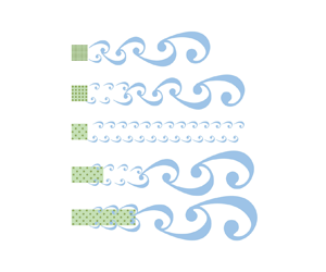
Flow visualizations were conducted to describe the wake structure and evaluate the mixing onset, supporting the velocity measurements. Red dye and green dye were simultaneously injected at two corners of the trailing edge (figure 2). A high-resolution camera (Sony FDR-AXP55,  $3480 \times 2160$ pixels) was placed around 5 m above the flume to cover the whole region downstream of the patches. Yellow coloured grid lines with a 20 cm interval regarding both $x$ and $y$ directions at the bottom were used to provide a distance reference. Light-emitting diodes were positioned along the glass flume wall to illuminate the observed region, which can avoid water surface light reflections. Videos with 25 frames per second were recorded over 1 min for all cases, starting at the beginning of the dye injection (examples with a 20 s stationary-stage capture can be found in the supplementary movies available at https://doi.org/10.1017/jfm.2023.156). Considering the shedding period of a Kármán vortex is $8$–
$8$– $13$ s from Liu et al. (Reference Liu, Hu, Lei and Nepf2018) and our observations, the collection duration (1 min) was enough to cover several vortex formations. To estimate the shedding frequency of the vortex street ( $\,f_{dye})$ and steady wake length ( $L_{d1}$, where the subscript ‘ $d$’ indicates estimation from dye experiments) from the videos, images with the same time interval (1 s) were extracted for analysis (figure 3). The time interval between two consequent vortices shedding to the same position (e.g. outermost) was recorded as the shedding period, $T_d$ (figure 4). Then, the vortex frequency can be estimated from the average of all observed values, $f_{dye}= 1/T_d$. The distance from the downstream end of the patch to the point where the two streaks of dye merge was defined as $L_{d1}$. The lengths extracted from all images were averaged to eliminate the oscillation of the mixing point due to the alternation of the vortex. The uncertainty was estimated from the standard deviation of the values measured from each image. To ensure water clarity for dye visualization, water in the tank was replaced after each two experimental runs.

Figure 3. Dye visualization experiment. The impact of (a) solid volume fraction for  $L/W = 2.22$, (b) patch length for $\varPhi = 0.013$. Flow is from top to bottom (red arrow). The dye was injected near the corners of the trailing edge. The yellow lines mark 20 cm intervals in both $x$ and $y$ directions (yellow arrows). The white arrows indicate the steady wake length ( $L_{d1}$).

Figure 4. The estimation of Kármán vortex shedding period,  $T_d$; (a) $t = t_0$, (b) $t = t_0 + T_d/2$, (c) $t = t_0 + T_d$.
For the analysis of velocity measurements, the distance from the patch leading edge ( $x = 0$) to the position where the velocity achieves an equilibrium or starts to increase within the patch is defined as the measured interior adjustment length, $L_{a,m}$, (the subscript ‘ $m$’ here indicates the estimation from measurements). The steady wake length, $L_1$, is estimated from the longitudinal velocity profile as the distance from the downstream end of the patch to the position where the velocity begins to increase, indicating the formation position of the vortex street. The distance from the end of the steady wake region to a point where the velocity is recovered to 90 % of the mean upstream velocity, $U_\infty$, is defined as the wake recovery (wake decay) length $L_2$. The uncertainty of the evaluation of $L_1$ and $L_2$ is induced by the measurement spacing at that point. Here $U_1$ is the mean streamwise velocity at $x = L + L_1$, $y = 0$ and $U_2$ is the unchanged mean streamwise velocity in the non-vegetation region at the corresponding $x$ transect. The recovery rate (spatial acceleration) of the recovery region is defined as $(U_\infty -U_1)/L_2$. Similarly, $U_{e1}$ is the mean streamwise velocity at the central point of the patch trailing edge, and $U_{e2}$ is defined as the mean streamwise velocity at the open area at the same transect, i.e. $x = L$. All these velocities defined here were time averaged and measured at mid-depth of the water height. These definitions have been largely discussed and used by Chen et al. (Reference Chen, Ortiz, Zong and Nepf2012) and Zong & Nepf (Reference Zong and Nepf2012). The previous attentions, however, were focused on circular patches with comparable longitudinal and transverse length dimensions. For an elongated patch, the similar definitions are applied herein. All these definitions can be seen in figure 1.
3. Results
3.1. Hydrodynamic adjustment
Time-averaged streamwise velocities ( $\bar {u}$) along the channel centreline were measured under different patch solid volume fractions ( $\varPhi$, figure 5) and aspect ratios ( $L/W$, figure 6). To highlight the degree of impact caused by the presence of the patches, the velocity is normalized by upstream unaffected velocity ( $U_\infty$). It is clearly observed that the flow velocity has been adjusted in response to the blocking effect of a porous patch centred on the flume. Streamwisely, the velocity adjustment, initially occurring in front of the patch, displays an apparent decay through the patch and recovered in the wake area for all scenarios. The velocity drop is more sensitive to $\varPhi$ rather than to $L$. In other words, under the same $L$, an earlier and larger drop occurs at a larger $\varPhi$ (figure 5) but the velocity drops presented in the longitudinal velocity profiles nearly show an overlap for cases under the same $\varPhi$ (figure 6).

Figure 5. Longitudinal profiles of velocity for patches under the same length: (a)  $L = 0.1$ m, (b) $L = 0.2$ m, (c) $L = 0.6$ m, (d) $L = 1.0$ m, (e) $L = 1.40$ m. The dashed lines indicate the trailing edges of the patches. The longitudinal velocity is measured at the patch centreline, $y = 0$.

Figure 6. Longitudinal profiles of velocity for patches under the same  $\varPhi$: (a) case A ( $\varPhi = 0.009$), (b) case B ( $\varPhi = 0.013$), (c) case Bw ( $\varPhi = 0.013$), (d) case C ( $\varPhi = 0.020$), (e) case D ( $\varPhi = 0.040$). The dashed lines with corresponding colour of the case indicate the trailing edges of the patches with $L = 0.10$ m, 0.20 m, 0.60 m, 1.0 m, 1.4 m from left to right. The longitudinal velocity is measured along the patch centreline, $y = 0$.
After entering the patch, the whole patch falls within the adjustment region when  $L < L_a$, where the velocity keeps decreasing with the same rate under the same $\varPhi$ (figure 6). However, larger $\varPhi$ leads to a more pronounced velocity drop (figure 5). Moreover, $L_a$ becomes smaller as $\varPhi$ increases, which follows the observations of flow adjustment within a long patch (Rominger & Nepf Reference Rominger and Nepf2011). For longer patches, velocity adjustment completes within the patches, indicating $L \geq L_a$, and once the velocity minimum is achieved, the flow shifts to re-acceleration. This velocity recovery behaviour within the patch attributed to lateral KH vortex interaction is similar to the results of some cases reported by Rominger & Nepf (Reference Rominger and Nepf2011). Clearly, a larger $\varPhi$ tends to promote the re-acceleration within the patches, indicating the enhancement of the parallel lateral KH vortex interaction under larger $\varPhi$. In particular, a larger $W$ tends to effectively attenuate the velocity decay process due to mass conservation (B cases, $W$ = 0.09 m versus Bw cases, $W$ = 0.21 m, figure 5). Furthermore, widening the patch tends to increase $L_a$, which is also consistent with the statistical relationship of $L_a$, $C_Da$ and $W/2$ developed by Rominger & Nepf (Reference Rominger and Nepf2011). Theoretically, widening the patch decreases the aspect ratio ( $L/W$) that should be comparable to the scenarios of shortening the patch under a fixed width, which is analysed in the following.
For a constant  $\varPhi$, the overlapping region of the velocity adjustment under variable $L/W$ (as shown in figure 6) ends as the velocity starts to recover, indicating that the downstream flow dynamics is negligibly influential to the upstream region for a vegetation-patch flow. This also confirms the analytical solution, developed by Liu et al. (Reference Liu, Shan, Sun, Yan and Yang2020), of the longitudinal velocity profile along a near-bank patch. As noted above, as the patch continuously elongates, the velocity decay tends to cease from the after-patch region ( $x > L$) to the in-patch region ( $x < L$) with a continuous reduction of the minimum velocity, opposite to widening the patch. As observed above (Bw cases in figure 5), the patches with larger $W$ tend to present a larger minimum velocity though longer decay length. The essence for this behaviour is that the increase in aspect ratio ( $L/W$) promotes the interior flow adjustment.
The interior adjustment lengths observed from longitudinal profiles of streamwise velocity,  $L_{a,m}$, agree well with those calculated from the formula developed by Rominger & Nepf (Reference Rominger and Nepf2011), $L_{a,c}$ (figure 7). This consistency confirms no sidewall effect on the in-patch velocity adjustment. It is also noted that $L_a$ is independent of $L$ (Rominger & Nepf Reference Rominger and Nepf2011; Chen et al. Reference Chen, Jiang and Nepf2013; Kim et al. Reference Kim, Kimura and Shimizu2015), thus, each $L_{a,m}$ is averaged among cases with varying $L$ but the same $\varPhi$ once $L \geq L_a$ (i.e. case D stands for the mean value for cases D3–D5 in table 2). For case A ( $\varPhi$ = 0.009), the fully developed region only occurs in case A5 ( $L$ = 1.4 m) and its $L_{a,m} = 1.3 \pm 0.1$ m. Thus, case A presents a relatively larger deviation mainly due to insufficient measurement density. Flow within case Bw is not fully developed, according to either calculated $L_{a,c}$ or measured $L_{a,m}$, which is not plotted in figure 7.

Figure 7. Comparison between  $L_{a,c}$ and $L_{a,m}$. The dashed lines indicated the 80 % confidence intervals.
Table 2. Measured parameters. Here VK and KH indicate the presence (Y) or absence (N) of a Kármán vortex street and KH vortex street, respectively.

The wake structure at  $x = L + L_1$ for cases with different lengths is evaluated by the lateral profiles of $\bar {u}/U_\infty$ given in figure 8 and normalized Reynolds shear stress (- $\overline {u'v'}/u_{*}^2$, where $u_{*}$ is the friction velocity) in figure 9. When the patch length is smaller than the interior adjustment length, velocity keeps decreasing within the patch, thus, steady wake velocity decreases as patch length increases, i.e. larger velocity deficit (figure 8a). However, when the interior velocity adjustment is completed within the patch (interior adjustment length < patch length), the velocity presents a recovery region after the interior adjustment region. Because interior adjustment length is constant under the same vegetation density and patch width, a larger patch length results in a longer velocity recovery region. The velocity deficit appears to reduce due to the velocity recovery. Thus, a peak velocity deficit presents when the patch elongates downstream (figure 8b). In summary, the velocity deficit may keep growing (before full interior velocity adjustment) or present a peak (after full interior velocity adjustment) as the patch length increases, consistent with the results shown in figure 6. Additionally, if the peak exists, the peak will present earlier (under smaller patch length) when $\varPhi$ increases. This is because vegetation density may speed up the interior velocity adjustment and shorten the interior adjustment length. For instance, velocity deficit peaks at $L = 1.0$ m for case B ( $\varPhi = 0.013$) while it shifts to $L = 0.6$ m for case D ( $\varPhi = 0.020$). The peak of the normalized Reynolds shear stress is located outside the patch edge, which is a signature of a shear layer (figure 9). The maximum normalized Reynolds shear stress value shows a monotonically increasing trend as the patch length increases, except for the cases from D4 to D5 (figure 9b). For a sparse patch with relatively low density (cases A1, B1, C1) and/or short length (cases A2, B2), no peak presents in the lateral profile of the normalized Reynolds shear stress, implying no shear layer formed.

Figure 8. Lateral profiles of  $\bar {u}/U_\infty$ for (a) case A ( $\varPhi = 0.009$), (b) case D ( $\varPhi = 0.040$) at $x = L + L_1$. Owing to the symmetry about the centreline ( $y/W = 0$), measurements were only taken across half of the flume width (from the centreline to a sidewall, $0 < y/W < 2.56$). The black dashed line shows the patch edge.

Figure 9. Lateral profiles of normalized Reynolds stress - $\overline {u'v'}/u_*^2$ for (a) case B ( $\varPhi = 0.013$), (b) case D ( $\varPhi = 0.040$) at $x = L + L_1$. The black dashed line shows the patch edge.
3.2. Wake vortex structure
According to dye visualization, the increase in  $\varPhi$ ( $0.009$– $0.040$) gradually encourages the formation of wake vortex streets (figure 3a). The obvious alternation observed at $\varPhi = 0.020$ (case C2) is weakened for lower $\varPhi$ (i.e. $\varPhi = 0.013$, case B2) and even cannot be detected when $\varPhi$ = 0.009 (case A2). This oscillation with no alternation in case A2 is likely attributed to local shearing and transverse diffusion (Chen & Jirka Reference Chen and Jirka1995; Uijttewaal & Booij Reference Uijttewaal and Booij2000), while the wake instability is not eventually attained. Meanwhile, the increase in $\varPhi$ tends to accelerate the mixing of free parallel streams, shortening the steady wake region ( $L_{d1}$). In fact, the effect of the solid volume fraction on the wake vortex street observed herein is consistent with the existing works such as Zong & Nepf (Reference Zong and Nepf2012) and Liu et al. (Reference Liu, Hu, Lei and Nepf2018). Similar to $\varPhi$ enhancement, patch elongation can enhance the turbulent behaviour from local shearing and self-diffusion (case B1, $L/W = 1.11$) to small-scale transverse wake oscillations (case B2, $L/W = 2.22$). Furthermore, the horizontal extent (size) of the vortices (indicated by dye) is further enhanced by the continuous growth in $L/W$ and $\varPhi$, but this growth seems to be suppressed by the water depth. This indicates that the horizontal size of the wake structure is controlled by both streamwise and spanwise dimensions of the patch (aspect ratio) as well as patch density.
Some deviations can be observed between dye measured  $L_{d1}$ and velocity measured $L_1$ in figure 10, though they are generally consistent. For small $L_1$ (or $L_{d1}$), the deviation may be caused by the initial velocity of the injected dyes. Thus, some distance is needed for the dye to adjust to the ambient flow condition, which delays the mixing of the dyes (i.e. $L_{d1} > L_1$). However, for larger $L_1$ (or $L_{d1}$), the mixing point is possibly a result of the diffusivity of the dyes rather than the vortex shedding, leading to a larger difference. Furthermore, the $L_{d1}$ estimated by eye detection also causes some uncertainties. The vortex frequency estimated from dye visualization ( $\,f_{dye}$) ranges from 0.13 to 0.20 Hz. For clarity, these statistical parameters and results are summarized in table 2.

Figure 10. Comparison between  $L_1$ and $L_{d1}$. Here $L_1$ is the length of the steady wake measured from the longitudinal profile of $\bar {u}$ at the patch centreline; $L_{d1}$ is measured from dye images and defined as the point at which the dye traces meet at the centreline. The dashed lines indicated the 80 % confidence intervals.
The formation and coherence of the wake vortex characteristics can be described by the power spectral density of velocity (Bouris & Bergeles Reference Bouris and Bergeles1999; Park et al. Reference Park, Lee, Jeon, Hahn, Kim, Kim, Choi and Choi2006). The power spectral density of spanwise velocity ( $S_{vv}$) distributions along the patch centreline under varying $L/W$ and $\varPhi$ are presented and compared in figure 11. The dashed lines indicate the leading and trailing edges of the patch. The presence of the wake vortex street is indicated by a definite peak at low frequency $f_{VK} = 0.12$– $0.19$ Hz after the patch, consistent with those estimated from dye visualization ( $\,f_{dye}$) (table 2). A similar vortex shedding frequency ( $0.08$– $0.22$ Hz) has been observed for circular patches (Zong & Nepf Reference Zong and Nepf2012; Hu et al. Reference Hu, Lei, Liu and Nepf2018; Liu et al. Reference Liu, Hu, Lei and Nepf2018). For the low $\varPhi$ = 0.009 (i.e. case A), an apparent low-frequency peak arises in the spectra distribution while $L/W \geq 6.67$ (case A3–A5), indicating that patch elongation can trigger the formation of the wake vortex street. Under higher $\varPhi$, the aspect ratio required for the initiation of the wake vortex street will be lower, for instance, the wake vortex street occurs when $L/W \geq 4.76$ and 2.22 for $\varPhi = 0.13$ (cases B and Bw) and 0.020 (case C), respectively. Furthermore, the low-frequency peak occurs for all aspect ratios investigated here ( $L/W \geq 1.11$) for the high $\varPhi = 0.040$ (case D), evidencing the domination of high $\varPhi$ for vortex street formation.

Figure 11. Power spectra ( $S_{vv}$) along the patch centreline ( $y = 0$). The dashed lines indicate the leading edge and trailing edge of the patch. Note that the width ( $W$) for the Bw cases is 0.21 m and 0.09 m for cases A–D.
In addition, the starting point of the peak migrates from the far-downstream region to directly behind the patch as  $L/W$ (e.g. case C2 to C3) and $\varPhi$ (e.g. case B3 to C3) increase, indicating the shortening of $L_1$. With sufficient $L/W$ and $\varPhi$, the peak even occurs within the patch with similar frequency, implying the presence of a Kármán-like structure (due to the interaction of KH vortex streets along two patch side edges). This indicates that the formation of the Kármán vortex street may be related to KH vortex streets, which will be discussed in § 4.2. However, due to the resistance induced by the vegetation stems, the intensity of this in-patch Kármán-like structure is weaker than the after-patch Kármán vortex street. After the patch, once the peak appeared, it decays during travelling downstream, indicating the decline of the wake vortex structure.
Turbulence theory indicates that the vortex characteristic length is inverse to the vortex frequency (Pope Reference Pope2000; Huai et al. Reference Huai, Xue and Qian2015). In this experiment, the peak experiences a slightly smaller frequency (not obvious in figure 11, but summarized in table 2) and a stronger peak (shown in darker red in figure 11) under a larger  $L/W$ and $\varPhi$, demonstrating the enhancement of the vortex street. This promotion becomes less significant under high $L/W$ and $\varPhi$, likely due to the limitation of the water level. This observation is consistent with that shown in the dye visualization. According to Taylor's frozen turbulence assumption with the local time-averaged velocity ( $U_1$) as the convection velocity, the vortex wavelength (vortex spacing) can be estimated to be $L_x = U_1/f_{VK} = 0.08$– $0.29$ m (table 2). The vortex spacing shows a reverse trend to the velocity difference ( $U_2-U_1$), indicating that a higher velocity gradient leads to smaller vortex spacing. It demonstrates again that the vortex characteristics (frequency, vortex space, strength, etc.) are highly affected by the combined effects of patch aspect ratio and solid volume fraction.
4. Discussion
4.1. Wake structure related to patch density and aspect ratio
Our experimental measurements of hydrodynamic fields around a centre-channel finite patch illustrate how flow velocity adjustment and wake structure respond to the vegetation patch under different cumulative resistance. The patch cumulative resistance is defined as the combined effect of the solid volume fraction ( $\varPhi$) and aspect ratio ( $L/W$), the latter of which has not yet drawn enough attention in previous studies. However, the aspect ratio of the vegetation patch may vary significantly in nature due to vegetation colonization dynamics and different types of aquatic vegetation morphology (Gurnell Reference Gurnell2014; Gran et al. Reference Gran, Tal and Wartman2015; Biggs et al. Reference Biggs, Nikora, Gibbins, Fraser, Green, Papadopoulos and Hicks2018; Yamasaki et al. Reference Yamasaki, de Lima, Silva, Preza, Janzen and Nepf2019). The increase in patch density and aspect ratio can both decrease the pore velocity and, thus, increase the main flow velocity by meeting the balance between momentum flux, high drag and gravitational force in the patch. This enhances the velocity difference or gradient transversely, thereby promoting flow instability in the wake. However, it is identified that the global response of flow to these two factors are in essence distinct due to the shifting of the interaction between the patch and flow. From the perspective of momentum conservation, patch elongation affects the flow structure by expanding the reach of its source effect instead of intensifying this effect. In contrast, the increasing patch density could locally enhance the drag force and dispersive stress on the local flow.
Beyond the trailing edge, a steady wake region can be raised for short and sparse patches, where momentum transport is dominated by advection effect (Zong & Nepf Reference Zong and Nepf2012; Kim, Kimura & Park Reference Kim, Kimura and Park2018). The steady wake length ( $L_1$) would be shortened with an early onset of vortex street. Wake vortex street can be found directly downstream of the patch (i.e. $L_1$ = 0) when $L > L_a$ under large $\varPhi$ (e.g. case D3) or large $L/W$ (e.g. cases A4, A5, B4, B5), or a combination of $\varPhi$ and $L/W$ (e.g. cases C3, D4, D5). According to figure 12(a,b) and table 2, both $U_1/U_\infty$ and $L_1/W$ decrease as $\varPhi$ increases within uncertainty. For the A cases ( $\varPhi$ = 0.009), both $U_1/U_\infty$ and $L_1/W$ show a continuous decrease trend as $L/W$ increases, while $U_1/U_\infty$ presents a recovery trend for other cases with higher density ( $\varPhi > 0.009$, i.e. cases B, C, D). The unsteady wake length ( $L_2$) is dependent on both the velocity recovery rate, $(U_\infty -U_1)/L_2$, and initial velocity deficit, ( $1-U_1/U_\infty$), at the wake vortex initiation point. The velocity recovery rate describes the rate of momentum input outside the wake while the initial velocity deficit describes the momentum required for full recovery. However, these two factors are interdependent and further complicate this issue. The unequal contributions of turbulence and velocity difference lead to a non-monotonic trend of $L_2$ to $\varPhi$ and $L/W$. Regarding the influence of the patch width, Bw cases with a width of 0.21 m present larger $L_1$ and $L_2$, a smaller velocity difference as well as recovery rate compared with B cases with a width of 0.09 m, indicating that patch width may have a negative effect on the generation of the vortex street. From the aspect ratio perspective, widening the patch performs like shortening the patch. However, only two patch widths are investigated here (not shown in the figure), a more detailed study with varying patch widths is recommended to confirm this finding.

Figure 12. The impact of  $\varPhi$ (i) and aspect ratio ( $L/W$, (ii)) on (a) normalized steady wake length, $L_1/W$, (b) normalized steady wake velocity, $U_1/U_\infty$, (c) wake recovery rate, $(U_\infty -U_1)/L_2$, (d) wake recovery length, $L_2$.
4.2. Coexistence between KH vortex street and wake vortex street
According to the observations in the current experiment (figure 11) and previous studies (Rominger & Nepf Reference Rominger and Nepf2011), two parallel KH vortex streets tend to be triggered due to flow instability along the lateral interfaces. Therefore, the correlation between the KH vortex streets and the wake vortex streets is of great interest. A straightforward way is to use a dye tracer to track the vortex evolution, for example, releasing dye tracers simultaneously along the patch edge and at the wake. However, this method is not effective due to the strong dispersion of dye tracers within water flows. Alternatively, the frequency of the two kinds of vortices may be another indicator to imply their connection.
Similar to the Kármán vortex description, the presence of a KH vortex can be determined through the velocity power spectra ( $S_{vv}$) distribution along the patch lateral edge ( $x = 0 - L$, $y = W/2$, figure 13). The dashed lines in the figures indicate their perspective interior adjustment length ( $L_a$). As shown in figure 13, a peak in $S_{vv}$ distribution demonstrates the initiation of the KH vortex (White & Nepf Reference White and Nepf2007; Caroppi et al. Reference Caroppi, Gualtieri, Fontana and Giugni2020; Proust & Nikora Reference Proust and Nikora2020; Yan et al. Reference Yan, Duan, Wai, Li and Wang2022). Specifically, when approaching $L_a$, an instability structure starts to form (indicated by yellow in figure 13). Then, over $L_a$, KH vortex streets can be observed (indicated by red in figure 13), which is consistent with the study of Rominger & Nepf (Reference Rominger and Nepf2011). As the flow travels downstream, the enhanced velocity gradient at the patch lateral edge and weakened flow diversion contribute to the generation of a KH vortex street. This evolution will be intensified through the momentum exchange between the parallel KH vortex streets across the patch width (Rominger & Nepf Reference Rominger and Nepf2011), given by the stronger peaks at the B cases ( $W = 0.09$ m) relative to the Bw cases ( $W = 0.21$ m). Moreover, the presence of these peaks also complies with the occurrence of in-patch peaks (figure 11). Therefore, the Kármán-like structure within the patch is proved to be a result of the interaction of the two parallel KH vortex streets. This in-patch Kármán-like structure will persist after the patch as a Kármán vortex street. Based on the analysis of the results presented in figure 14, when a KH vortex occurs, a peak presents at $f_{KH} = 0.12$– $0.17$ Hz in $S_{vv}$, with an average of 0.14 Hz, consistent with the mean value of $f_{VK}$ = 0.15 Hz for the patch-scale Kármán vortex street, indicating that the KH vortex does have some similarity with the Kármán vortex.

Figure 13. Power spectra ( $S_{vv}$) along the lateral edge of the patch ( $x = 0 \sim L, y = W/2$). The dashed lines indicate the interior adjustment region ( $L_a$). Note that the width ( $W$) for the Bw cases is 0.21 m and 0.09 m for cases A–D.

Figure 14. Comparison between  $f_{VK}$ and $f_{KH}$. Here $f_{VK}$ is the frequency of the von Kármán vortex and $f_{KH}$ is the frequency of the KH instability. Both are measured from velocity power spectra. The solid line indicates $f_{VK} = f_{KH}$ and the dashed lines indicate the 80 % confidence intervals.
Furthermore, the results of the normalized Reynolds shear stress at  $x = 0-L$, $y = W/2$ for all cases are shown in figure 15. The normalized shear Reynolds stress at the end of the trailing edge shows an increasing trend as the aspect ratio and solid volume fraction increase, indicating the formation and growth of the KH vortex. This result is consistent with the peak values presented in the velocity power spectra above. However, when the length of case D ( $\varPhi = 0.040$) extends from $L$ = 1.0 m to 1.4 m, a sudden drop occurs, which is mainly caused by the strong interaction between two KH coherent structures developed along the parallel edges of the patch. This interaction leads to the formation of an in-patch Kármán-like vortex, which results in vortex intensity dissipation and velocity recovery as indicated in figures 5 and 6. This Kármán-like vortex has also been observed in the study of cylinders in tandem (Hosseini et al. Reference Hosseini, Griffith and Leontini2020). Moreover, this in-patch Kármán-like structure may explain why natural patches may not keep elongating downstream unrestrictedly but present an equilibrium length. Meanwhile, there exists a threshold value for normalized Reynolds shear stress, $-\overline {u'v'}/u_*^2$ (shown by the dashed line in figure 15), indicating the presence of a KH vortex street. More importantly, according to figure 15, a Kármán vortex will certainly be detected if a KH vortex presents, but a Kármán vortex can also form in the absence of a KH vortex. Therefore, here we consider that a KH vortex is a positive but not necessary condition for Kármán vortex initiation.

Figure 15. Normalized Reynolds stress at the position of  $(x, y) = (L, W/2)$. The dashed line indicates the threshold value for the normalized Reynolds stress of the presence of the KH vortex. Here ‘VK’ indicates wake vortex street; ‘KH’ indicates KH vortex street; ‘Y’ indicates yes/presence; ‘N’ indicates no/absence.
4.3. Wake vortex street formation thresholds
The generation of the wake vortex street may significantly impact the flow velocity distribution, scalar convection and dispersion, sediment deposition and morphodynamics in the wake (Follett & Nepf Reference Follett and Nepf2012; Zong & Nepf Reference Zong and Nepf2012; Liu et al. Reference Liu, Hu, Lei and Nepf2018). Therefore, a threshold indicator of the wake vortex street is desirable. Considering the available implementations for different scenarios, three groups of threshold parameters are identified based on the results and findings above.
It has been noted that the initiation and growth of large-scale coherent structures are related to the velocity asymmetry imposed by factors such as the topographic forcing in the transition region of the compound channel (Dupuis et al. Reference Dupuis, Proust, Berni and Paquier2017; Proust et al. Reference Proust, Fernandes, Leal, Rivière and Peltier2017), and multilayered density stratification (Caulfield et al. Reference Caulfield, Peltier, Yoshida and Ohtani1995). Similarly, the cessation of the wake vortex street has been shown to be related to the velocity difference (or gradient) induced by the porous patch because a high-velocity bleed flow can prevent the shear layers developing along two sides to reach each other. Intuitively, the parameter combination of  $U_1$ and $U_2$ (see definition in figure 1) at the wake vortex onset location is available for the threshold identification following Zong & Nepf (Reference Zong and Nepf2012). That is, when ( $U_2-U_1$) is too small, wake instability is unlikely to be triggered to form wake vortex streets. According to our experiments, a distinct vortex street appears when $U_1/U_2 <$ 0.5, which is different from the result ( $U_1/U_2 < 0.35$) from experiments conducted by Zong & Nepf (Reference Zong and Nepf2012) and numerical experiments by Chang & Constantinescu (Reference Chang and Constantinescu2015) regarding a circular patch (i.e. $L/W = 1$).
In addition to vegetation density as stated in previous studies, the wake instability has been found to be related to the patch aspect ratio ( $L/W$) based on our experiments. Under the same density investigated in this study, the vortex generation is promoted by patch length ( $L$) and suppressed by patch width ( $W$). Therefore, an integrated non-dimensional threshold value can be determined as $U_1/U_2 \times (L/W)^{-1}$, which is more appropriate for the threshold identification. Therefore, a threshold map for the wake vortex generation can be formed as shown in figure 16. Using a linear boundary $U_1/U_2 \times (L/W)^{-1} = 0.31$, no vortex street will be detected within the shaded area, while vortex street can be identified within the non-shaded area (figure 16a). This threshold incorporating the effect of the aspect ratio can express well the results of existing works (Zong & Nepf Reference Zong and Nepf2012) that are special cases of this expression. Alternatively, we can also use $(U_2-U_1)/U_\infty$ to represent the normalized velocity difference (figure 16b). In this case, the non-dimensional parameter is defined as $(U_2-U_1)/U_\infty \times L/W$ and it shifts to 0.84. That is, the vortex street occurs when $(U_2-U_1)/U_\infty \times L/W > 0.84$.

Figure 16. Aspect ratio ( $L/W$) versus velocity difference (a) $U_1/U_2$; (b) $(U_2-U_1)/U_\infty$ at $x = L + L_1$. The shaded area indicates the absence of the wake vortex street according to the threshold value.
Although the impact of patch length on velocity adjustment has been considered in  $U_1$, $L$ incorporated here is a consideration for the impact of the KH instability rather than a normalization purpose. Under a low-density patch with sufficient length, the reduced velocity within the patch enhances the lateral velocity gradient as travelling downstream. This strengthened velocity gradient may trigger the presence of KH instability. Before the generation of an in-patch Kármán-like vortex due to the interaction of the KH vortex, the formed KH instability has positive effects on the wake vortex street formation as well. For example, case C1 presented a close but slightly higher velocity gradient ( $(U_2-U_1)/U_\infty /W = 5.6\,{\rm m}^{-1}$) than that in case Bw4 $((U_2-U_1)/U_\infty /W = 4.7\,{\rm m}^{-1})$, but the wake vortex presents after case Bw4 rather than case C1. It is possibly caused by the energy contributed by the KH instability formed along the patch lateral edges in case Bw4, indicated by yellow in figure 13, even though it is weak. In addition, in the last case in the experiment of Zong & Nepf (Reference Zong and Nepf2012), with $(U_2-U_1)/U_\infty /W = 4.3\,{\rm m}^{-1}$ (where $D = 0.12$ m is the $W$ in this case), no wake vortex occurs, though its velocity gradient is higher than that of the vortex-generated case Bw3 $((U_2-U_1)/U_\infty /W = 3.6\,{\rm m}^{-1})$ in our experiment. Thus, the length of the patch should be incorporated into the threshold indicator to consider the positive contribution from the KH instability.
From a viewpoint of practical implementation, the sampling of  $U_{e1}$ and $U_{e2}$ at the cross-section of the trailing edge ( $x = L$) is much easier compared with $U_1$ and $U_2$ by locating the onset of vortex initiation ( $x = L + L_1$). Chen et al. (Reference Chen, Ortiz, Zong and Nepf2012) demonstrated that there existed some relationship between $U_1$ and $U_{e1}$. In this sense, we also seek another threshold in the form of $U_{e1}$ and $U_{e2}$. Similar to the above manipulation, a threshold map can be established for wake vortex street prediction as shown in figure 17. The map implies that the vortex street forms at $U_{e1}/U_{e2} \times (L/W)^{-1} <$ 0.35 (except for case D1) or $(U_{e2}-U_{e1})/U_\infty \times L/W > 0.55$.

Figure 17. Aspect ratio ( $L/W$) versus velocity difference (a) $U_{e1}/U_{e2}$; (b) $(U_{e2}-U_{e1})/U_\infty$ at $x = L$. The shaded area indicates the absence of the wake vortex street according to the threshold value.
Previous studies have reported that the solid volume fraction ( $\varPhi$) of the porous obstacle can also be a simple indicator for vortex street generation. According to the study of Castro (Reference Castro1971), the vortex street ceases to form after a slim perforated plate ( $L/W \ll 1$) when $\varPhi <$ 0.8. For a circular porous array ( $L/W = 1$), Zong & Nepf (Reference Zong and Nepf2012) reported that the cessation occurs at $\varPhi < 0.04$, which is very close to the limit ( $\varPhi < 0.05$) found in the numerical modelling by Nicolle & Eames (Reference Nicolle and Eames2011). The inconsistent observations are due to the overlook of the impact of aspect ratios. A smaller aspect ratio leads to a higher critical value. This is because $\varPhi$ only considers the local hydraulic resistance while the patch dimensions consider the reach of the hydraulic resistance. Considering the cumulative effect of patch dimensions, the patch aspect ratio, $L/W$, is incorporated to be $\varPhi \times L/W$. In the present experiments, increasing the cumulative hydraulic resistance (by $\varPhi$ or $L/W$), through altering the velocity shear in the wake, could play a critical role in promoting the formation of wake vortex streets.
For a patch of rigid emergent cylinders in aligned rectangular configurations with comparable streamwise and spanwise length scales (cases A1–D1, with  $L = 0.10$ m and $W = 0.09$ m, $L/W = 1.11$), the transition occurs at $\varPhi = 0.020$– $0.040$, which is close but slightly smaller than those observed in Nicolle & Eames (Reference Nicolle and Eames2011) and Zong & Nepf (Reference Zong and Nepf2012). When the patch elongates downstream, the transition occurs at $\varPhi = 0.013$– $0.020$ for cases with $L/W = 2.22$, which complies with our inference herein. Moreover, for $L/W > 2.22$, threshold values for $\varPhi$ are less than 0.009. Therefore, another threshold map ( $\varPhi \times L/W > 0.045$) considering the cumulative resistance caused by $\varPhi$ and $L/W$ is established for wake vortex street prediction as shown in figure 18. However, this threshold will cease to hold true when $\varPhi$ is so low that velocity recovers before the end of the patch, which is not considered in this study. Therefore, the validity of this threshold map may be limited to a certain range of patch density and dimensions, which needs a broader-range investigation. It is better to understand the wake structure together with the velocity gradient. Moreover, this threshold map was developed for a single rectangular vegetation patch of rigid emergent cylinders in an aligned configuration. Hydraulic resistance is expected to be higher in staggered configurations with less flow through patches, resulting in the onset of the vortex street for lower solid volume fractions. Besides, the flexibility, submergence ratio and the presence of leaves in real plants are not considered either, further investigations are expected.

Figure 18. Aspect ratio ( $L/W$) versus solid volume fraction ( $\varPhi$). The shaded area indicates the absence of the vortex street according to the threshold value.
In consequence, the following three kinds of thresholds have been established for identifying the formation of wake vortex streets in a channel with vegetation patches of rigid emergent cylinders in an aligned configuration under different densities and aspect ratios, which can be used alternatively based on the availability of corresponding parameters in different scenarios.
(i) Quantified by velocity scales measured at the end of the steady wake region ( $x = L + L_1$), a Kármán vortex street will appear when
(4.1)or\begin{equation} U_1/U_2 \times (L/W)^{{-}1} < 0.31 \end{equation}(4.2)\begin{equation} (U_2 - U_1)/U_\infty \times L/W > 0.84. \end{equation}
$x = L + L_1$), a Kármán vortex street will appear when
(4.1)or\begin{equation} U_1/U_2 \times (L/W)^{{-}1} < 0.31 \end{equation}(4.2)\begin{equation} (U_2 - U_1)/U_\infty \times L/W > 0.84. \end{equation}(ii) Quantified by velocity scales measured at the patch trailing edge (
$x = L$), a Kármán vortex street will appear when
(4.3)or\begin{equation} U_{e1}/U_{e2} \times (L/W)^{{-}1} < 0.35 \end{equation}(4.4)\begin{equation} (U_{e2}-U_{e1})/U_\infty \times L/W > 0.55. \end{equation}(iii) Quantified by patch characteristics, a Kármán vortex street will appear when
(4.5)\begin{equation} \varPhi \times L/W > 0.045. \end{equation}


In this connection, this study forms an essential extension with substantial contribution to this scientific research. However, there still exists some limitations in this study. Firstly, only two widths were investigated in this case, the variations caused by varying patch widths and patch blockage ratios ( $W/B$) have not been systematically studied. Secondly, the influence of the KH instability on wake structure has not been fully understood. An interesting future test would be expected to split the patch in half with a solid dividing barrier/plate along the patch centreline to prevent any lateral ’communication’ of KH vortices across the patch (essentially forming two independent shear layers and weaker intensity) and see how it would affect KH vortex formation, especially for narrow cases. Thirdly, the combined impact of vegetation density ( $\varPhi$) and patch aspect ratio ( $L/W$) was investigated under the aligned configuration of rigid and emergent stems with uniform cylinder rods in this experiment. Hydraulic resistance is expected to vary under different configurations. Lastly, in a natural system the configuration will be even more complicated, features may evolve over time and space, with a random configuration, irregular patch shape and a wider range of stem sizes and densities. For instance, the threshold developed in our study failed to predict the formation of the wake vortex after the natural, submerged patch with flexible leaves investigated in the field study of Biggs et al. (Reference Biggs2019). This may attribute to the restriction of this threshold to rigid, emergent vegetation patches with no leaves or the limited measured reach in their study (Biggs et al. Reference Biggs2019). Therefore, the flexibility, submergence ratio, the presence of leaves in real plants and the varying flow conditions, such as incoming velocity and water depth, in natural aquatic systems need to be further systematically investigated.
5. Conclusions
This study experimentally addressed the importance of both solid volume fraction ( $\varPhi$) and aspect ratio (length/width, $L/W$) to the hydrodynamic behaviour, particularly wake formation and structure, in response to a centre-channel porous rectangular patch under aligned configuration of rigid and emergent stems. A total of 25 experimental runs under varying $\varPhi$ and $L/W$ were carefully designed and carried out for investigation, with the aid of rigorous velocity measurements and dye visualizations. The experimental results firmly demonstrated the significant impact of the patch aspect ratio on wake structure, and complements previous experimental works on wake structures behind circular porous patches with comparable longitudinal and transverse dimensions.
It is observed that the solid volume fraction indicates the local hydraulic resistance, of which influence can be immediately felt by the local velocity adjustment, shown as the velocity gradient. A larger solid volume fraction leads to a faster velocity drop. However, patch dimensions determine the reach of the resistance. A larger patch width delays the flow diversion laterally, leading to an adverse effect on the interior velocity adjustment, while the patch length controls the distance of the velocity drop and triggers the generation of the KH instability along the patch lateral edges. Therefore, a larger patch length and vegetation density may lead to a higher velocity reduction, but patch width presents the opposite impact. The combined effect of solid volume fraction and patch aspect ratio is representative of cumulative hydraulic resistance. It affects the wake structure by changing the bleed flow velocity and initiating a KH instability at the patch trailing edge. Moreover, the two parallel KH vortex streets formed along the lateral edges of the patch under sufficiently high aspect ratios tend to interact with each other, leading to velocity recovery owing to transverse momentum input, especially for a smaller width. In contrast to the scenarios of high  $\varPhi$ producing wake flow instability due to inducing a large transverse velocity difference, the patch elongation through triggering KH vortex streets may impose an extra impact on the patch wake vortex street structures.
Furthermore, we attempted to explore the threshold for the generation of wake vortex streets based on previous and current observations. Three non-dimensional parameter-based threshold maps considering different indicator combinations were established. Based on the characteristic velocity scales ( $U_1$ and $U_2$) at the onset location of the vortex street ( $x = L + L_1$), the wake vortex street would appear when $U_1/U_2 \times (L/W)^{-1} < 0.31$ or $(U_2 - U_1)/U_\infty \times L/W > 0.84$. Based on the characteristic velocity scales ( $U_{e1}$ and $U_{e2}$) at the trailing edge of the patch ( $x = L$), the wake vortex street would occur when $U_{e1}/U_{e2} \times (L/W)^{-1} < 0.35$ or $(U_{e2}-U_{e1})/U_\infty \times L/W > 0.55$. In addition, based on solid volume fraction ( $\varPhi$) and aspect ratio ( $L/W$), the wake vortex street would occur when $\varPhi \times L/W > 0.045$. These three threshold maps can be alternatively used for theoretical interpretation and implementation by considering the parameter availability under different test scenarios. The first two threshold maps are likely to be applied to a wider range of patch configurations (and potentially also to flexible vegetation) since they are based on characteristic velocity scales in the wake. Further work is needed to determine whether the third threshold map based on the solid volume fraction applies more broadly, since stem alignment, flexibility and surface area (skin friction) may also be important factors leading to patch hydraulic resistance, velocity gradients and vortex street formation.
Supplementary movies
Supplementary movies are available at https://doi.org/10.1017/jfm.2023.156.
Funding
This research work was supported by the Research Grants Council (RGC) of the Hong Kong University Grants Committee (UGC) under project no. 15200719; the Hong Kong Polytechnic University under project no. 4-ZZNF; and the National Natural Science Foundation of China under project no. 51909178.
Declaration of interests
The authors report no conflict of interest.


 Open access