2.1. Governing equations

Large-eddy simulation within a weather research and forecasting (WRF) model was developed and validated to simulate thermal buoyant plumes (Bhaganagar & Bhimireddy Reference Bhaganagar and Bhimireddy2020b; Bhimireddy & Bhaganagar Reference Bhimireddy and Bhaganagar2021). A thorough performance assessment of WRF has been conducted to accurately resolve the micro-scale turbulence (Bhaganagar & Bhimireddy Reference Bhaganagar and Bhimireddy2017; Bhimireddy & Bhaganagar Reference Bhimireddy and Bhaganagar2018a,Reference Bhimireddy and Bhaganagarb; Bhaganagar & Bhimireddy Reference Bhaganagar and Bhimireddy2020a). For the sake of completeness, the numerical framework is presented here. The governing equations are the compressible Euler equations with eddy viscosity and gravitational forces as follows:

(2.1a)\begin{gather} \dfrac{\partial\rho}{\partial t} +\dfrac{\partial\rho u_i}{\partial x_i} =0, \end{gather}

(2.1b)\begin{gather}\dfrac{\partial\rho u_i}{\partial t} +\dfrac{\partial \rho u_j u_i}{\partial x_j} ={-}\dfrac{\partial p}{\partial x_i} +\dfrac{\partial\tau_{ij}}{\partial x_j} -\delta_{3i}\rho g, \end{gather}

(2.1c)\begin{gather}\frac{\partial\rho\theta}{\partial t} +\dfrac{\partial \rho u_j\theta}{\partial x_j} = \dfrac{\partial}{\partial x_j}\rho Pr_t^{{-}1}\mu_t\dfrac{\partial\theta}{\partial x_j} -\delta_{i3}\dfrac{h_0 g}{C_p}, \end{gather}

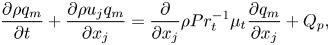(2.1d)\begin{gather}\frac{\partial\rho q_m}{\partial t} +\dfrac{\partial \rho u_j q_m}{\partial x_j} = \dfrac{\partial}{\partial x_j}\rho Pr_t^{{-}1}\mu_t\dfrac{\partial q_m}{\partial x_j}+Q_p, \end{gather}

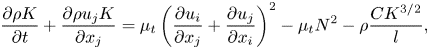(2.1e)\begin{gather}\dfrac{\partial\rho K}{\partial t} +\dfrac{\partial \rho u_j K}{\partial x_j} = \mu_t\left(\dfrac{\partial u_i}{\partial x_j}+\dfrac{\partial u_j}{\partial x_i}\right)^2 -\mu_t N^2 -\rho\dfrac{C K^{3/2}}{l}, \end{gather}

where $\rho$ is the mixture density, $u_i$ is the velocity component in the $i$ direction, $\theta$ is the potential temperature, $q_m$ is the mass fraction of the $m$th species and $K$ is the modelled TKE. Also, $p$ is the pressure, $\tau _{ij}$ is the modelled stress tensor given by $\tau _{ij}=\mu _t(\partial _j u_i+\partial _i u_j-(2/3)\delta _{ij}\partial _k u_k$, $\delta$ is the Kronecker delta function, $C_p$ is the specific heat capacity at constant pressure and $h_0$ is the heat flux applied at the source only. The gravitational term $g$ is considered as a body force, which acts in the negative vertical direction. The eddy viscosity, $\mu _t$, is defined as $\mu _t\equiv C_k l\sqrt {K}$ where $C_k=0.1$ and $l$ is a length scale given as $l=\min [(\Delta x\Delta y \Delta z)^{1/3}$, $0.76\sqrt {K}/N]$ if $N>0$, otherwise $l=(\Delta x\Delta y\Delta z)^{1/3}$. The Brunt–Väisälä frequency, $N$, is computed as $N^2=(g/\theta )\partial _3\theta$.

Further, $Pr_t$ is the turbulent Prandtl number which is defined as $Pr_t^{-1}=1+2l(\Delta x\Delta y \Delta z)^{-1/3}$. From observations, $Pr_t\gtrsim 0.66$ along the centreline in all plumes.

Ideal gas is assumed in the equation of state, and therefore, potential temperature can be related in the equation of state, $p=p_0(\rho R\theta /p_0)^{\gamma }$, where $R$ is the specific gas constant and $\gamma$ is the specific heat ratio. In the following discussion, horizontal and vertical velocities, $u_1$ and $u_3$, will be presented as $u$ and $w$. For the spatial directions $x_1$ and $x_3$, they will be replaced by $x$ and $z$.

Besides the small-scale turbulence modelled in (2.1e), large-scale quantities, including density, velocities, temperature and mass fraction, are resolved in the conservation laws (2.1a–d). Note that density ($\rho$) is calculated based on the local mass fraction. In addition, the system simulates buoyancy effects without the Boussinesq assumption.

2.2. Physical problem

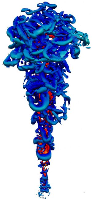
The physical problem that is being investigated in this study is as follows: the physical domain is filled with ambient fluid that is at rest and maintained at a constant temperature. A circular region of the source at the bottom boundary with diameter $D({=}400\ {\rm m})$ is heated with a constant surface heat flux ($h_0$). The heating causes a temperature difference between the surface and the ambient fluid and convection is initiated (see figure 1). In this work, three different gases are studied: heated air (thermal), heated methane (${\rm CH}_4$) and heated sulphur dioxide (${\rm SO}_2$). In addition to the surface heat flux, for ${\rm CH}_4$ and ${\rm SO}_2$ cases, the gases are released with a constant surface density flux at the source. Chemical reactions and phase change are not considered in the presented simulations.

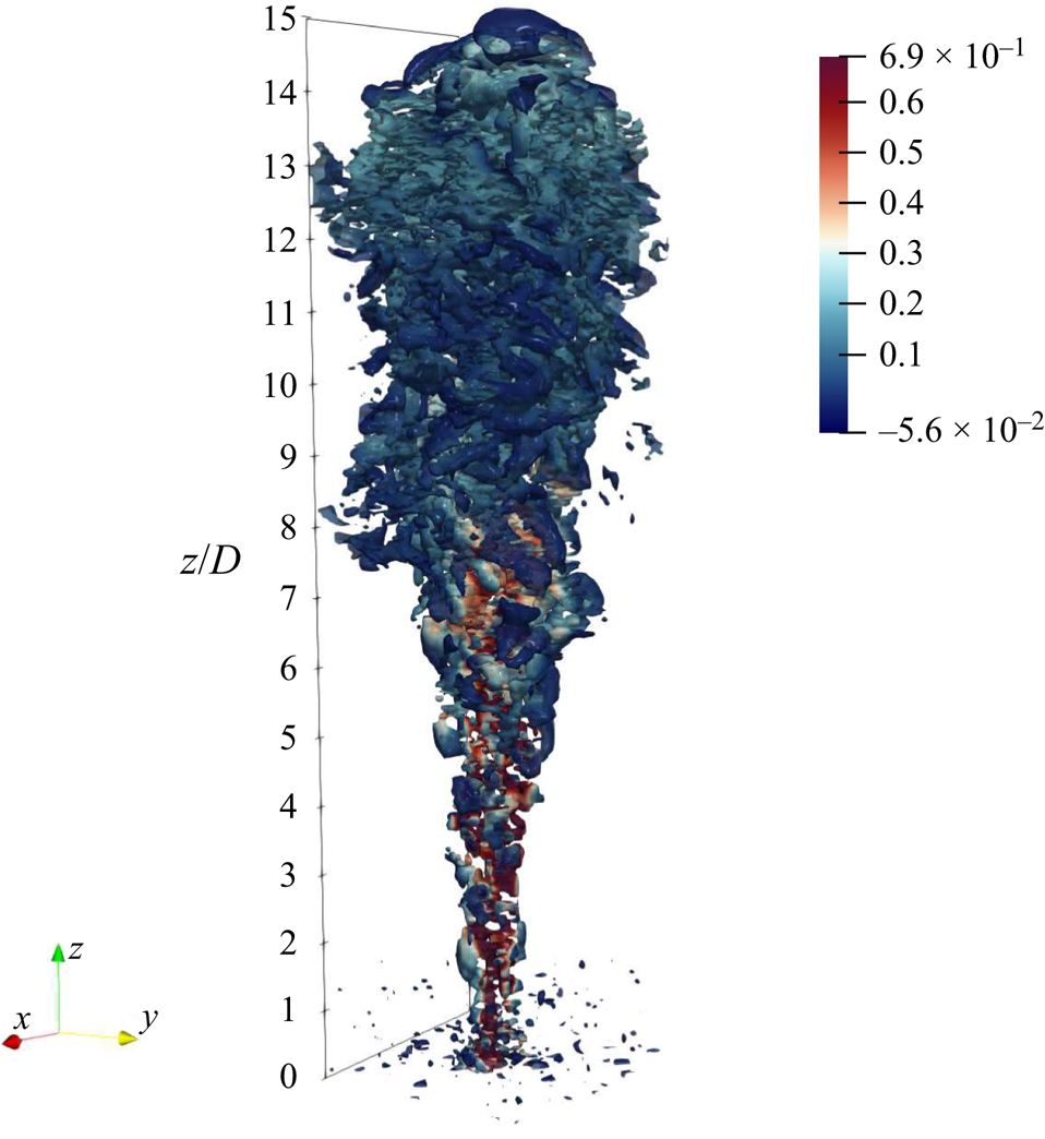
Figure 1. The $\lambda _2$ vortex criterion (Jeong & Hussain Reference Jeong and Hussain1995) of a thermal turbulent buoyant plume coloured with ambient temperature subtracted from potential temperature.

A representation of turbulent buoyant plume is shown in figure 1, in which the $\lambda _2$-criterion is plotted. A buoyancy source at the bottom of the domain generates an upward buoyancy flux which induces entrainment of the ambient fluid as the plume rises. Turbulence velocity fluctuations and temperature fluctuations are generated by the plume.

The coordinate system is Cartesian, and the horizontal directions are represented by the $x$ and $y$ axes and the vertical direction is represented by the $z$ axis. The domain size, $(L_x,L_y,L_z)=(10D,10D, 17.5D)$. The initial conditions are the hydrostatic pressure conditions, $\partial _3 p=-\rho g$, and the equation of state with reference state specified at the sea level. Additionally, zero velocity conditions are imposed throughout the domain due to quiescent ambient conditions. Periodic boundary conditions are imposed on the horizontal (transverse) direction. At the top of the domain, a constant pressure is specified based on hydrodynamic relations and a no-slip condition is imposed at the bottom.

The simulations have been performed for seven different cases. The details of the cases are provided in table 1. Cases 1–5 represent the release of heated air referred to as the thermal plume. The surface heat flux $h_o$ for these cases varies in the range $0.0044\unicode{x2013}0.024\ {\rm kg}\ {\rm s}^{-3}$. Cases 6 and 7 are for ${\rm CH}_4$ and ${\rm SO}_2$ released with $h_o$ of $0.024\ {\rm kg}\ {\rm s}^{-3}$.

Table 1. Scaled parameters of the source and the plume: $R$ is the specific gas constant, $h_0$ is the heat flux of the source; $\Delta \rho =(\rho _0-\rho _{\infty })/\rho _{\infty }$ is the density difference between the source ($\rho _0$) and the ambient ($\rho _{\infty }$); $g_0'$ is the initial reduced gravity at the source defined as $g_0'=(T_0-T_{\infty })g/T_0$, where $T_0$ is the temperature at the source and $T_{\infty }$ is the ambient temperature; $z^*$ is the streamwise location of maximum mean velocity normalized by $D$; $l^*$ is the half-width of the plume at $z^*$ normalized by $D$. The following dimensionless quantities are measured at $z^*$: $Re=\bar {w}l^*/\nu$ with viscosity obtained from the air temperature while $Re_{t}=w''l^*/\nu _t$ with eddy viscosity $\nu _t$; $Re_{sgs}=\sqrt {TKE_{sgs}}\Delta z/\nu _t$, where $sgs$ represents subgrid scale; $R_K$ is the ratio of subgrid-scale TKE to the resolved TKE; $M=\bar {w}/c$, where $c$ is the speed of sound; $M_t=w''/c$; $Fr=w/\sqrt {g_0'D}$ and $At=(\rho _0-\rho )/(\rho _0+\rho )$.

The Reynolds and Froude numbers are calculated based on time-averaged flow variables after the plumes reach the stationary state. The dimensional parameters are $h_0$, $g_0'$, $\Delta \rho$ and $R$; the resulting non-dimensional parameters are the Reynolds number and the Froude number. The resolution for all the simulations is $100^2\times 700$. The grid-independence test increased the resolution from $40^2\times 250$ to $200^2\times 1400$, and found that the temporal-spatial evolution of both centreline velocity and the plume height saturate at $100^2\times 700$. The simulations have been validated by comparing the mean centreline velocity and plume height against experimental measurements (Ai, Law & Yu Reference Ai, Law and Yu2006) and with theoretical analysis (Bhamidipati & Woods Reference Bhamidipati and Woods2017). Good agreements were obtained with those predictions in the literature. In addition, comparison between $100^2\times 700$ and $200^2\times 1400$ showed that the relative errors of the resolved vorticity are ${<}2\,\%$ and the error of the modelled dissipation is ${O}(10^{-6})$.

When buoyant plumes rise from their sources, their structures begin developing as the heat is transferred to the mean flows. Such energy transfer further results in the generation of TKE, thermodynamic fluctuations and other turbulent structures. Figure 2 shows the spatial distributions of mean flow and other turbulent variables along the centreline from case 5. Starting at the source, all the quantities have a monotonic increase and reach their maximum. Mean vertical velocity, $\tilde {w}$, peaks first at $z/D\approx 2$, followed by $\overline {\rho '^2}$ and $\widetilde {T'' w''}$ at $z/D\approx 3$. Finally, the vertical fluctuating velocity, $w''$, reaches its peak last at $z/D\approx 5$. The following discussion shows a strong dependence of the plume structures on these three characteristic locations. The values of $\widetilde {T''^2}$ and $\overline {\rho ' w''}$ show similar distributions to $\overline {\rho '^2}$ and $\widetilde {T'' w''}$, and therefore are not presented.

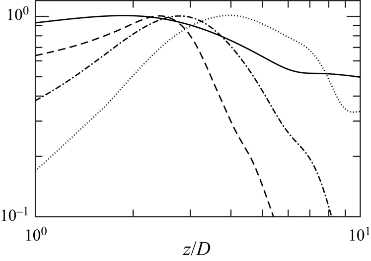
Figure 2. The axial distributions of mean axial velocity ($\bar {w}$, solid), density variance ($\overline {\rho '^2}$, dashed), vertical turbulent heat flux ($\widetilde {T' w''}$, dash-dotted) and axial Reynolds stress ($R_{33}$, dotted) along the centreline for case 5.

3.1. Spatial distributions

The notation used in this manuscript is as follows – for an instantaneous flow variable $q$, the Reynolds time-averaged quantify ($\bar {q}$) is defined as $\bar {q}=\varSigma _i^n q_i/n$, where, $n$ is the number of instantaneous time steps after the flow reached stationary state. Unless otherwise stated, the normalization has been performed based on the maximum value along the centreline. The symbol $^*$ denotes the normalized value with respect to the maximum value at the centreline. The Favre-averaged variable is defined as $\tilde {q}=\overline {\rho q}/\bar {\rho }$. The Favre-averaged fluctuations are, therefore, defined as $q''=q-\tilde {q}$. For the rest of the manuscript, fluctuations represent the Favre-averaged fluctuations. Tensor notation is used to represent all higher-order tensors. The Reynolds stresses, $R_{\alpha \alpha }$ are defined as $R_{\alpha \alpha }\equiv \widetilde {u''_{\alpha }u''_{\alpha }}$.

We begin the analysis by examining the axial distribution of axial ($R_{33}^*$) and horizontal ($R_{11}^*$) components of the TKE, as plotted in figure 3(a,b). Here, $R_{11}$ is the average from both transverse directions. since our data show that the plumes are axisymmetric. The existence of two plume distinct regimes – the initial and the mixing stages are evident. It should be noted that for starting plumes, the mean flow accelerates from rest and reaches a maximum velocity at around $2D-3D$ above the source. Meanwhile, TKE reaches its maximum near $z/D=5$. This stage ($z/D\lesssim 5$) is referred to as the initial stage. During the initial stage, turbulence (velocity fluctuations and thermodynamic fluctuations) is still developing and without significant radial expansion (see figure 1).

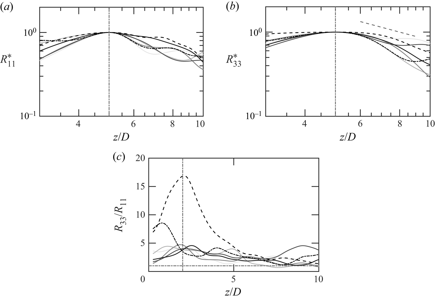
Figure 3. (a) Centreline distributions of $R_{11}$ normalized by the peak value. (b) Centreline distributions of $R_{33}$ normalized by the peak value. (c) Ratio of $R_{33}$ and $R_{11}$ at the centreline. Solid lines: thermal plumes (grey), methane (black, dashed) and sulphur dioxide (black, dash-dotted). Solid lines: thermal plumes, grey levels from light to dark correspond to case 1–5 in ascending order. Black dashed and dash-dotted lines represent methane and sulphur dioxide plumes, respectively. Grey dash-dotted lines: $z/D=2$ (vertical) and $R_{33}/R_{11}=1$ (horizontal).

The plume next enters the mixing stage in which the turbulence starts to decay; meanwhile, much more significant radial expansion is observed. This stage is referred to as the mixing stage. This occurs around $z/D > 5$. During the initial stages, both the components of the Reynolds stresses increase from the source value and reach their peak value at $z/D\approx 5$, beyond which they decrease exponentially with an exponent of $-1$ during the mixing stage. Even though a minor scatter exists in the mixing stage, the comprehensive analysis shows a consistent and monotonic decrease in the region from $z/D=5$ to $z/D=17.5$. Similar spatial trends have been observed for other thermal, ${\rm CH}_4$ and ${\rm SO}_2$ cases. There is no observable trend with Reynolds number. To further understand the differences between the components of the Reynolds stresses, the ratio of $R_{33}$ and $R_{11}$ is plotted in figure 3(c). Unlike $R_{33}$ and $R_{11}$ which peak at around $5D$, $R_{33}/R_{11}$ peaks at approximately $2D$ instead. Further ahead, this ratio decreases with height and it slowly approaches an asymptotic value of unity. This suggests a tendency towards isotropy. The approach-to-isotropy process indicates that, further away from the source, the two components of the Reynolds stresses are dominated by similar mechanisms.

For thermal plumes, monotonic increase with $Re$ and $Fr$ is observed in the maximum value of $R_{33}/R_{11}$. Such trends are reasonable as budget analysis will later reveal that buoyancy is a dominant mechanism in the Reynolds stress and dissipation is a counterpart. For species plumes, the difference can be realized through the Atwood number as high $At$ is associated with increasing mixing in buoyancy-driven flows (Luo et al. Reference Luo, Wang, Xie, Wan and Chen2020; Taha et al. Reference Taha, Zhao, Lamorlette, Consalvi and Boivin2022).

3.2. Budget analysis

To understand the mechanisms that control the Reynolds stresses, the budget equation for Reynolds stresses is presented next

(3.1)\begin{equation} \bar{\rho}\tilde{u}_k\dfrac{\partial R_{\alpha\alpha}}{\partial x_k} = P_B+P_S+\varPi+\epsilon+{M}+\mathcal{T}. \end{equation}

In (3.1), the left-hand term is the mean convection equation On the right-hand side, $P_B$ and $P_S$ are the production terms and $\varPi$ is the pressure dilatation, $\epsilon$ is the dissipation, $M$ is the mass-flux contribution and $\mathcal {T}$ is the summation of all transport terms. The explicit form of each term is given as follows:

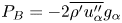(3.2a)\begin{gather} P_B ={-}{2\overline{\rho' u''_{\alpha}}g_{\alpha}} \end{gather}

(3.2b)\begin{gather}P_S ={-}2\bar{\rho} R_{\alpha k}\dfrac{\partial\tilde{u}_{\alpha}}{\partial x_k} \end{gather}

(3.2c)\begin{gather}\varPi = 2\overline{p'\dfrac{\partial u''_{\alpha}}{\partial x_{\alpha}}} \end{gather}

(3.2d)\begin{gather}\epsilon ={-}2\overline{\sigma_{\alpha k}'\dfrac{\partial u''_{\alpha}}{\partial x_k}} \end{gather}

(3.2e)\begin{gather}M = 2\overline{u''_{\alpha}}\dfrac{\partial\overline{\sigma_{\alpha k}}}{\partial x_k} \end{gather}

(3.2f)\begin{gather}\mathcal{T} ={-}\dfrac{\partial\bar{\rho}\overline{u''_{\alpha}u''_{\alpha} u''_k}}{\partial x_k} -2\dfrac{\partial\overline{p' u''_{\alpha}}}{\partial x_{\alpha}} +2\dfrac{\partial\overline{\sigma_{\alpha k}'u''_{\alpha}}}{\partial x_k}. \end{gather}

The three terms in $\mathcal {T}$ are turbulent, pressure and viscous transport. The derivation of (3.1) is provided in Appendix A.

To get a better understanding of the contribution of the axial vs the radial components to the TKE, we study the axial and the horizontal components of the TKE budget separately. In addition, TKE is further decomposed into the vertical ($R_{33}$) and horizontal ($R_{11}$) components.

The budget terms of $R_{33}$ along the centreline are plotted in figure 4(a). The results are shown for case 5 (thermal plume). Each term is obtained using the resolved quantities, except the dissipation, which adopts both the resolved and modelled terms. Among all the terms, buoyancy production is the most dominant mechanism, and pressure dilatation, production by mean flows, transport terms and dissipation are also important. Only the mass-flux contribution is negligible. Due to axial symmetry, production only contains $R_{33}\partial _3 \tilde {u}_3$ along the centreline. The spatial evolution along the centreline can be divided into three major regions: buoyant production, pressure-dilatation and dissipation terms increase from the source to $z/D\approx 3$ (as marked by vertical dash-dotted line where $\overline {\rho '^2}_{max}$ occurs), and they peak around $z/D=3$. Meanwhile, the transport changes sign from positive (towards the source) to negative (away from the source). As the plume continues to ascend from $z/D\approx 3$ to $z/D\approx 5$ (as marked by the vertical dashed line where $R_{33,max}$ occurs), the contributions from buoyancy and dilatation reduce. It is interesting to note, however, that, at the same time, production by mean flows reaches its maximum in this region. During the mixing stage ($z/D\gtrsim 5D$), all the terms decrease and they tend to zero. Comparison of the pressure dilatation and the transport shows that the two terms are counteracting each other far away from the source. Negative pressure dilatation in the initial stage suggests that energy is being transferred out of $R_{33}$ through pressure and dilatation due to strong anisotropy. As the turbulent flows approach an isotropic state in the mixing stage, pressure dilatation is reduced significantly.

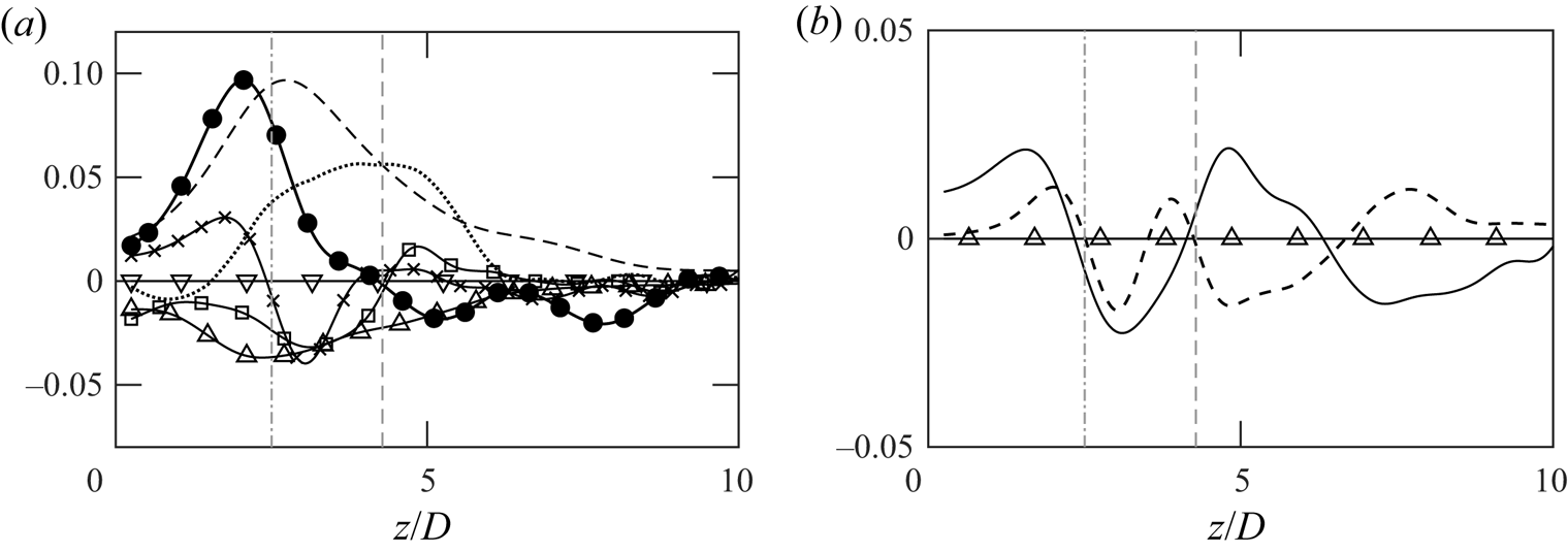
Figure 4. (a) Budget of $R_{33}$ from case 5 (thermal plume): convection ($\bullet$); $P_B$ ($--$); $P_S$ ($\cdots$); $\varPi$ ($\square$); $\epsilon$ ($\Delta$); $M$ ($\nabla$); $\mathcal {T}$ ($\times$). (b) Decomposition of transport: turbulent transport (dashed); pressure transport (solid); viscous transport ($\Delta$). Vertical grey lines: $\overline {\rho '\rho '}_{max}$ (dash-dotted) and $R_{33,max}$ (dashed).

Decomposition of the transport terms is shown in figure 4(b), and it indicates that viscous transport is negligible while turbulent and pressure transports have similar distributions during the initial stage ($z/D<5$) near the source. Such trends change completely during the mixing stage, After the plume enters the mixing stage, the two terms start acting against each other. As a result, the overall transport contributions become negligible in the mixing stage. Similar results regarding the budget terms are observed in different gas plumes. Overall, the budget analysis of thermal plumes shows an interesting result that axial velocities are strongly related to density fluctuations as multiple terms change their trends at the peak of $\overline {\rho '^2}$. More discussion regarding such a discovery will be provided in the following sections.

To further understand the most dominant term, the buoyant production terms for the different thermal plumes (cases 1–5) are plotted in figure 5(a). With an increasing heat flux at the source, the buoyancy contributions increase correspondingly. For all the cases, the peak production occurs near the corresponding location of $\overline {\rho '^2}_{max}$ regardless of the source conditions. In figure 5(b), the buoyancy contributions in thermal, methane and sulphur dioxide plumes with identical heat release are plotted. The peak location shifts toward the source for heavier gases (smaller specific gas constant $R$). In addition, the heavier is the gas, the higher is the buoyant production. For the same heat release from the source, heavier plumes contain more energy per unit volume, and hence result in stronger buoyancy contributions. For the heavier plumes, the peak location closer to the source is due to the stronger gravitational forces exerted on the gases.

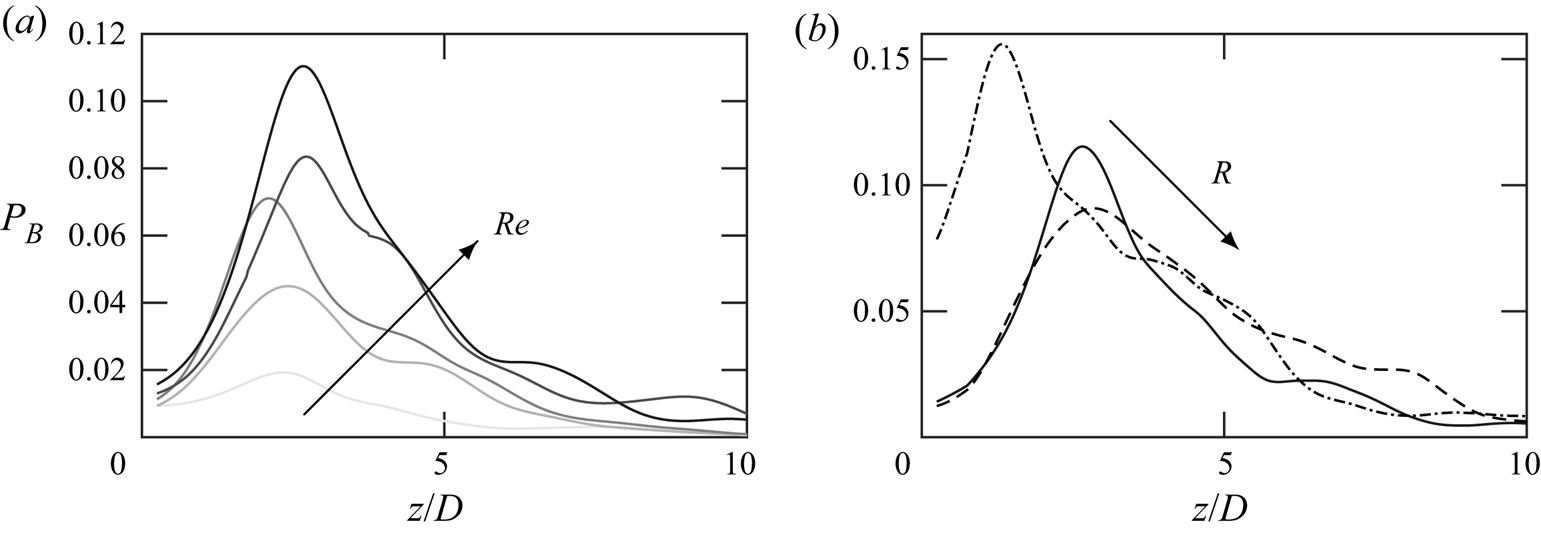
Figure 5. (a) Buoyant production of $R_{33}$ in thermal plumes; (b) buoyant production of $R_{33}$ in plumes with different species. Same colours as in figure 3.

Next, the budget analysis of $R_{11}$ is presented in figure 6. Unlike $R_{33}$, there is no production term. The figure shows that the transport of $R_{11}$ is strongly dominated by pressure dilatation and dissipation. The dominant pressure dilatation in $R_{11}$ shows that energy is redistributed to $R_{11}$ through pressure and dilatational effects. Similar to $R_{33}$, $R_{11}$ also shows significant dependence on density fluctuations. Both the dominant terms peak near the maximum of $\overline {\rho '^2}$ near $z/D\approx 3$. A strong dependence on dilatation motions is shown in the transport of $R_{11}$ during the initial stage.

Figure 6. Budget of $R_{11}$ from case 5: convection ($\bullet$); pressure dilatation ($\square$); mass-flux contribution ($\nabla$); transport ($\times$); dissipation ($\Delta$).

Overall, the TKE budget analysis at the centreline reveals that TKE production is initiated by buoyancy production (closer to the source) in the initial regime of the plume; $R_{ij}\tilde {u}_{i,j}$ becomes important in turbulence generation during the mixing stage. Energy is transferred from the mean flow to axial Reynolds stress. Pressure redistribution is the key process that distributes the energy from the axial to the radial components of Reynolds stress. A complex relation of the pressure transport and turbulent transport drives the mixing of the axial Reynolds stresses. The turbulent transport of the radial Reynolds stress, which will be shown later, plays an important role in the entrainment process.

Budget analysis along the centreline provides a basic understanding on the turbulent development within the plumes. However, as the plumes enter the mixing stage, significant radial developments are observed. Figure 7 shows the distributions of $R_{33}$ budget terms along the transverse direction at different heights. Both production terms are still the dominant terms along the transverse direction; and peak turbulence production occurs radially away from the centreline. Off-centre peak during the developing stage ($z/D\leqslant 5$) is expected, and slowly disappears during the mixing stage ($z/D>5$).

Figure 7. Radial profiles of $R_{33}$ budget from case 5 (thermal plume): convection ($\bullet$); $P_B$ ($--$); $P_S$ ($-{\cdot }$); $\varPi$ ($\square$); dissipation ($\Delta$); $M$ ($\nabla$); vertical ($+$) and horizontal ($\times$) components of $\mathcal {T}$ at (a) $z/D\approx 2$ and (b) $z/D\approx 5$. Vertical grey dashed lines represent the boundary of the source.

The radial profiles of $R_{11}$ terms are shown in figure 8. Near the centreline, pressure dilatation and dissipation are the dominant budget terms. Further away from the centre, transverse transport dominates the budget terms and the direction of the transport is radially towards the centreline. This observation is consistent throughout the plumes at different heights and indicates that the turbulent transport terms are the main contributors to entrainment.

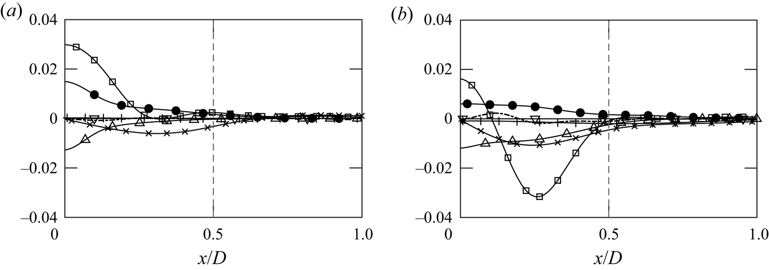
Figure 8. Radial profiles of $R_{11}$ budget from case 5 (thermal plume): convection ($\bullet$); $\varPi$ ($\square$); $M$ ($\nabla$); $\epsilon$ ($\Delta$); vertical ($+$) and horizontal ($\times$) $\mathcal {T}$ at (a) $z/D\approx 2$ and (b) $z/D\approx 5$. Vertical grey lines represent the boundary of the source.

To understand the influence of transport processes on the plume dynamics, the radial profiles of transverse transport terms (with the exception of molecular transport which is insignificant) at a height of $2D$, $5D$ and $10D$ above the source are plotted in figure 9. From the budget analysis of $R_{33}$, the transport is radially outwards near the source ($2D$). As the plumes transition from the initial to the mixing stage, the direction of transport reverses at $z/D\approx 5$. Near the plume top, i.e. at $z/D=10$, the transport term becomes negligible. For $R_{11}$, the radial pressure transport dominates the transport processes at all heights. The radial transport is mainly towards the centreline. Summing the transport processes, turbulence transport is the main mechanism for vertical mixing, while the pressure transport dominates the horizontal mixing processes. The mixing can thus be quantified in terms of turbulent and pressure transport for axial and vertical mixing, respectively.

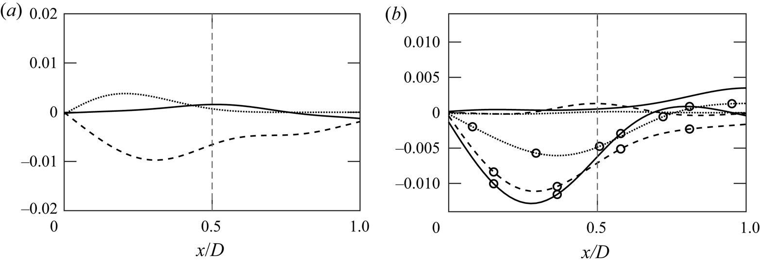
Figure 9. (a) Radial profiles of $R_{33}$ turbulent transport terms from case 5 (thermal plume) at $z/D\approx 2$ ($\cdots$), $z/D\approx 5$ ($--$) and $z/D=10$ ($-$). (b) Radial profiles of $R_{11}$ turbulent (lines) and pressure ($\circ$) transport from case 5 at $z/D\approx 2$ ($\cdots$), $z/D\approx 5$ ($--$) and $z/D=10$ ($-$).

3.3. The TKE spectra

In classical, inertia-dominated turbulence, the source of TKE production is at the large scale and the sink of the turbulence dissipation is at the small scale, and the energy is cascaded in the inertial regime and eventually in the dissipative regime. The spectral slope in the inertial regime follows the classical $-5/3$ power law. In atmospheric turbulence, and in thermally stratified turbulence, the existence of a buoyancy-dominated regime at low wavenumbers has been demonstrated, wherein, the spectral slope of the energy cascading follows the $-3$ power law. The LES study of Chen & Bhaganagar (Reference Chen and Bhaganagar2021) demonstrated, for the first time, that the energy spectrum for thermal plumes follows the $-3$ power law and the energy cascades from the low wavenumber buoyancy regime to the high wavenumber dissipative regimes. To further understand the difference between different species, the energy spectra of thermal, methane and sulphur dioxide plumes are presented at two different heights in figure 10. Here, $E_{uu}$ and $E_{ww}$ represent the energy spectra of horizontal and vertical velocity fluctuations. Similar to the thermal plumes, a buoyancy regime with $-3$ slope is observed in methane and sulphur dioxide plumes during both the initial and mixing stages. In addition, figure 10 also shows that plumes with lighter gases contain slightly more TKE. Overall, the energy spectra from different species have consistent energy containing buoyancy regimes in their spectra.

Figure 10. Spectra of vertical (black, $E_{ww}$) and transverse (grey, $E_{uu}$) velocities from thermal plume ($-$), methane ($--$) and sulphur dioxide ($-{\cdot }$) at (a) $z\approx 2D$ and (b) $z=10D$. Here, $k_h$ represents the horizontal wavenumber.

Following the proposal of a $-3$ buoyancy range from Lumley (Reference Lumley1964), multiple studies further suggested $E(\kappa )=c N^2 k^{-3}$ (Billant & Chomaz Reference Billant and Chomaz2001; Lindborg Reference Lindborg2006). In figure 11, the compensated spectra, $E_{ww}/(N^2 k_h^{-3})$ and $E_{uu}/(N^2 k_h^{-3})$, at $z/D=5$ from different plumes are plotted against the wavenumber. The asymptotic states are observed at high wavenumbers for all plumes. Those saturations are also captured when the spectra are presented at different heights for case 5 in figure 12. The plotted compensated spectra clearly show and support the buoyancy range with a $-3$ spectral slope. From the two figures, we can infer that the coefficient $c$, instead of being a universal constant, depends on the species and plume height. Further investigations are required to quantify the values of $c$.

Figure 11. Compensated spectra of (a) vertical velocity and (b) transverse velocity from thermal ($-$), methane (${\rm CH}_4$) and sulphur dioxide (${\rm SO}_2$) plumes at $z/D=5$. Same colours and lines as in figure 3.

Figure 12. Compensated spectra of (a) vertical velocity and (b) transverse velocity of thermal plume (case 5) at $z/D=2$ ($-$), $z/D=3$ ($--$), $z/D=5$ ($-{\cdot }$) and $z/D=10$ ($\cdots$).

4.1. Statistical scalings

The streamwise distributions of density and temperature variance, $\overline {\rho '^2}$ and $\widetilde {T''^2}$, along the centreline are shown in figure 13. To have a consistent discussion with the budget analysis, Favre averaging is adopted for temperature.

Figure 13. Centreline distributions of (a) $\overline {\rho '^2}$ and (b) $\widetilde {T''^2}$, each normalized by its maximum. Same lines as in figure 3. All distributions are aligned at $z/D=2$ (grey, dash-dotted).

In addition, the difference between the normalized $\widetilde {T''T''}$ and $\overline {T'T'}$ is $\overline {\rho 'T'}^2/\bar {\rho }^2\bar {T}^2\sim M_t^8$ (Donzis & Jagannathan Reference Donzis and Jagannathan2013). Such a difference is negligible under most atmospheric and engineering problems (Donzis & John Panickacheril Reference Donzis and John Panickacheril2020).

All distributions are normalized by the peak value of the variance. In this figure, the distributions are aligned at $z/D=2$ since the thermodynamic fluctuations have their peak at around $z/D\lesssim 3$. Similar to the Reynolds stresses, thermodynamic fluctuations increase monotonically from the source to the peak, beyond which they decrease exponentially with an exponent of $-2.5$. This is much faster compared with an exponent of $-1$ observed for the Reynolds stresses. As the decay occurs faster compared with Reynolds stresses, this indicates a faster decay of thermodynamic fluctuations with height compared with their velocity fluctuation counterparts. At around $z/D\approx 10$, the fluctuations of density and temperature are already two orders smaller than their peak values.

A different normalization is presented. Figure 14 shows the thermodynamic variances normalized by their local averages. A consistent exponent of $-2.3$ is observed for all the cases. A clear dependence on Reynolds number and specific gas constant is observed. With an increasing $Re$ or a decreasing $R$, thermodynamic fluctuations increase with respect to their local averages. However, significant differences exist in the normalized values between the plumes. The normalized variances with different source conditions reach an order of $100$. Such a dependence implies a stronger acoustic generation with compressibility effects, and those phenomena can have significant impacts on engineering systems and natural environments.

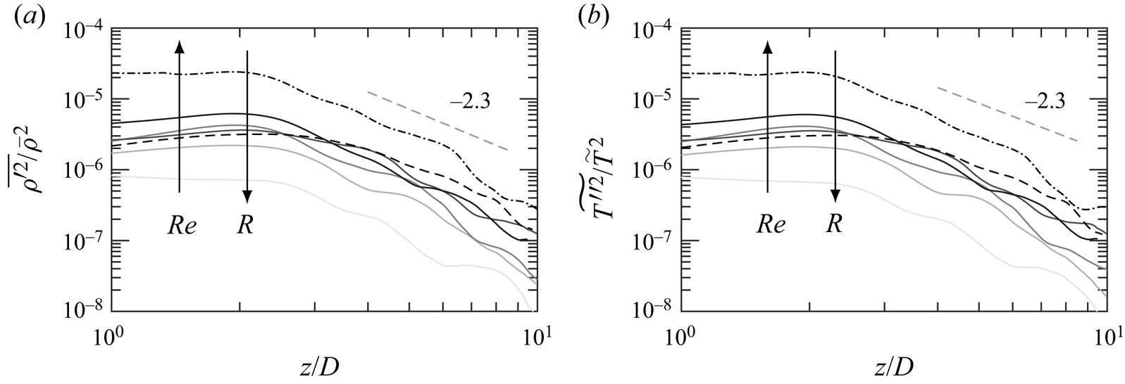
Figure 14. Centreline distributions of (a) $\overline {\rho '^2}/\bar {\rho }^2$ and (b) $\widetilde {T''^2}/\tilde {T}^2$. Same colours as in figure 3. All distributions are aligned at $z/D=2$ (grey, dash-dotted).

The radial profiles of $\overline {\rho '\rho '}$ at different heights are shown in figure 15(a). Near the source ($z/D=2$), an off-centre peak is observed. The peak decreases significantly with height and disappears before $z/D=3$. After the density fluctuations reach their peak near $z/D=3$, an obvious transverse development is observed and the profiles become wider. Figure 15(b) further shows the profiles at $z/D=5$ from different plumes. Despite having different heat releases, the five different thermal plumes have very similar distributions. In addition, the methane plume has slightly wider profiles. Similar to the centreline distributions, $\widetilde {T''T''}$ has very similar distributions to $\overline {\rho '\rho '}$ after normalization.

Figure 15. (a) Radial profiles of density variances at $z/D=2D$ ($-$); $z/D=3D$ ($--$); $z/D=5D$ ($-{\cdot }$); $z/D=10D$ ($\cdots$). (b) Radial profiles of thermal plumes ($-$); methane ($--$; sulphur dioxide ($-{\cdot }$). Solid lines: grey levels from light to dark represent cases 1–5 in ascending order; $^*$ represents the normalization by the local centreline values.

4.2. Budget analysis

To understand physical mechanisms that control the thermodynamic fluctuations, we first look at the transport of the density variance. The budget terms of $\overline {\rho '^2}$ are computed

(4.1)\begin{equation} \tilde{u}_j\dfrac{\partial\overline{\rho'^2}}{\partial x_j} = \mathcal{P}_{\rho}+P_{\rho}+\mathcal{T}_{\rho}+\varPi_{\rho}+{\rm \pi}_{\rho}. \end{equation}

Similar to (3.1), the term on the left-hand side of the equation is the convection. On the right-hand side of the equation, $\mathcal {P}_{\rho }$ and $P_{\rho }$ are the production by the mean flows and density gradient, respectively, $\mathcal {T}_{\rho }$ is the transport and $\varPi _{\rho }$ and ${\rm \pi} _{\rho }$ are the density dilatation connected with the mean flows and fluctuations, respectively. The explicit form of each term is provided as follows:

(4.2a)\begin{gather} \mathcal{P}_{\rho}={-}2\overline{\rho'^2}\dfrac{\partial\tilde{u}_j}{\partial x_j} \end{gather}

(4.2b)\begin{gather}P_{\rho}={-}2\overline{\rho' u''_j}\dfrac{\partial\bar{\rho}}{\partial x_j} \end{gather}

(4.2c)\begin{gather}\mathcal{T}_{\rho}={-}\dfrac{\partial\overline{\rho' \rho' u''_j}}{\partial x_j} \end{gather}

(4.2d)\begin{gather}\varPi_{\rho}={-}2\bar{\rho}\overline{\rho'\dfrac{\partial u''_j}{\partial x_j}} \end{gather}

(4.2e)\begin{gather}{\rm \pi}_{\rho}={-}\overline{\rho'^2\dfrac{\partial u''_j}{\partial x_j}}. \end{gather}

Figure 16(a) shows that the evolution of $\overline {\rho '^2}$ is solely dominated by $P_{\rho }$ and $\varPi _{\rho }$ while other terms are at least one order smaller in comparison. From the figure, we can understand that density fluctuations are generated through dilatation terms and diminished due to the turbulence production from density gradient term. Since density and the velocities are negatively correlated, $P_{\rho }$ is acting as a sink rather than as a source.

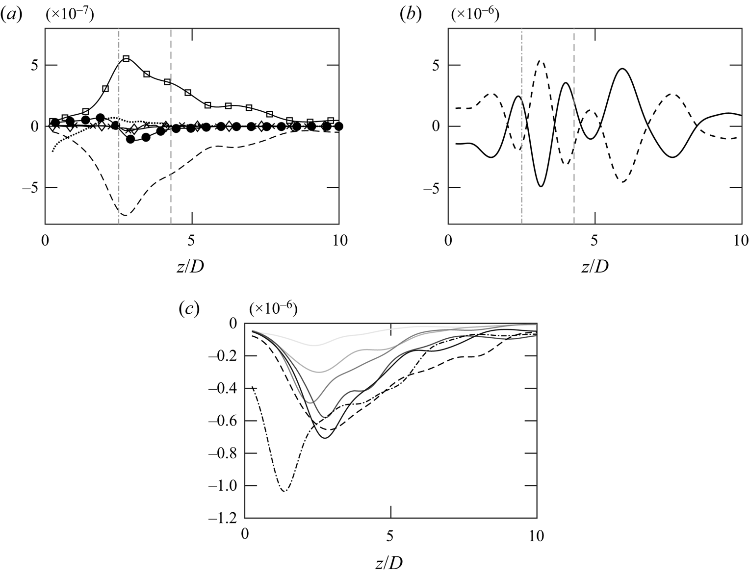
Figure 16. (a) Budget of $\overline {\rho '^2}$ from case 5: convection ($\bullet$); $\mathcal {P}_{\rho }$ ($\cdots$); $P_{\rho }$ ($--$); $\varPi _{\rho }$ ($\square$); ${\rm \pi} _{\rho }$ ($\diamond$); $\mathcal {T}_{\rho }$ ($\times$). (b) Distributions of vertical ($-$) and horizontal ($--$) components of $\varPi _{\rho }$. Vertical grey lines: $\overline {\rho '\rho '}_{max}$ (dash-dotted) and $R_{33,max}$ (dashed). (c) Distributions of $P_{\rho }$: thermal plumes, grey levels from light to dark correspond to cases 1–5 in ascending order. Black dashed and dash-dotted lines represent methane and sulphur dioxide plumes, respectively.

While the dilatation term is usually associated with compressibility effect, the effects on the presented plumes are considered small due to the low Mach numbers. Instead, density–velocity correlation, which exists in both $P_{\rho }$ and $\varPi _{\rho }$, is the main mechanism. The nearly perfect cross-correlation between $\rho$ and $w$ will be discussed in § 5.

Both of the dominant terms peak near $\overline {\rho '^2}_{max}$. The density dilatation ($\varPi _{\rho }$) can be further decomposed into vertical and horizontal components. The two components are plotted in figure 16(b). The horizontal and vertical components make opposite but similar contributions throughout the plume. The mirrored distributions of the two different dilatation components indicate that dilatational motions occur when the vertical and horizontal motions are unbalanced. Density fluctuations are generated during this re-distribution process when the flows are anisotropic. During the initial stage, significant contributions of $\varPi _{\rho }$ result from strong anisotropy. Such contributions are slowly reduced as the turbulent flows approach isotropy with an ascending plume. Overall, the main contribution for the density dilatation comes from the imbalance of fluctuations through $\rho\unicode{x2013}w$ cross-correlation. Figure 16(c) shows another important term, $P_{\rho }$, with different heat sources and gases. With the increasing heat release from the source, $P_{\rho }$ grows correspondingly; $P_{\rho }$ is also found to be more prominent in heavier gases. Although production from mean flow gradients was found to be important to Reynolds stresses, the analogous term, $\mathcal {P_{\rho }}$, is negligible in the transport of $\rho '$ in buoyant plumes.

The contributions from the pressure and viscous effects are present, hence more terms are involved in the transport of $\widetilde {T''^2}$. The budget analysis of $\widetilde {T''^2}$ is computed

(4.3)\begin{equation} \bar{\rho}\tilde{u}_j\dfrac{\partial\widetilde{T''^2}}{\partial x_j} = \mathcal{P}_T+P_T+\varPi_T+\epsilon_T+\mathcal{T}_T. \end{equation}

Besides the convection terms on the left side of the equation, $\mathcal {P}_{T}$ and $P_{T}$, on the right side of the equation, are the production from the mean flows and temperature gradient, respectively, $\varPi _T$ is the temperature dilatation connected with the pressure, $\mathcal {T}_T$ is the sum of all the transport terms and $\epsilon _T$ is the dissipation. The explicit form of those budget terms is given as

(4.4a)\begin{gather} \mathcal{P}_T={-}\dfrac{2}{C_v}\overline{pT''}\dfrac{\partial\tilde{u}_j}{\partial x_j} +\dfrac{2}{C_v}\overline{T''\sigma_{ij}}\dfrac{\partial\tilde{u}_i }{\partial x_j} \end{gather}

(4.4b)\begin{gather}P_T={-}2\bar{\rho}\widetilde{T'' u''_j}\dfrac{\partial \tilde{T}}{\partial x_j} \end{gather}

(4.4c)\begin{gather}\varPi_T={-}\dfrac{2}{C_v}\overline{pT''\dfrac{\partial u''_j}{\partial x_j}} \end{gather}

(4.4d)\begin{gather}\epsilon_T=\dfrac{2}{C_v}\overline{T''\sigma_{ij}\dfrac{\partial u''_i}{\partial x_j}} -\dfrac{2}{C_v}\overline{k_T\dfrac{\partial T''}{\partial x_j}\dfrac{\partial T}{\partial x_j}} \end{gather}

(4.4e)\begin{gather}\mathcal{T}_T={-}\dfrac{\partial\overline{\rho T''^2u''_j}}{\partial x_j} +\dfrac{2}{C_v}\dfrac{\partial}{\partial x_j}\overline{k_TT''\dfrac{\partial T}{\partial x_j}}, \end{gather}

where $C_v$ is the specific heat capacity at constant volume, $\mathcal {T}_T$ contains both turbulent and thermal transports and $\epsilon _T$ includes viscous and thermal dissipation.

The budget terms in (4.4) are shown in figure 17(a). Similar to $\overline {\rho '^2}$, the evolution of $\widetilde {T''^2}$ is dominated by the temperature dilatation and the production of temperature gradient terms.

Figure 17. (a) Budget of $\widetilde {T''^2}$ from case 5: convection ($\bullet$); $\mathcal {P}_T$ ($\cdots$); $P_T$ ($--$); $\varPi _T$ ($\square$); $\epsilon _T$ ($\Delta$); $\mathcal {T}_T$ ($\times$). (b) Distributions of vertical ($-$) and horizontal ($--$) components of $\varPi _T$. Vertical grey lines: $\widetilde {T''T''}_{max}$ (dash-dotted) and $R_{33,max}$ (dashed). (c) Distributions of $P_T$: thermal plumes, grey levels from light to dark correspond to cases 1–5 in ascending order. Black dashed and dash-dotted lines represent methane and sulphur dioxide plumes, respectively.

Section 5 will further show a very strong correlation between $T''$ and $w''$. The two dominant budget terms are therefore associated with cross-correlation rather than the compressibility.

In contrast to $\overline {\rho '^2}$, $P_T$ is functioning as a source rather than as a sink, and the dilatational motions are negative. However, the dilatation mechanisms are also significant in the initial stage in which turbulence is highly anisotropic, just as was observed in $\overline {\rho '^2}$. Further, decomposition of $\varPi _T$, as shown in figure 17(b), shows opposite distributions of vertical and horizontal dilatations. Similar to density, the dilatational effects occur in response to anisotropic motions and contribute to $\widetilde {T''^2}$. In figure 17(c), $P_T$ from different plumes is presented. The production increases with heat source and with increasing density difference between the source and the ambient fluid (i.e. heavier gases).

In addition to the centreline distributions, budget terms are also compared in the transverse directions. Figure 18 shows the dominant terms of $\overline {\rho '\rho '}$ and $\widetilde {T''T''}$. Consistent with the centreline distributions, $P_{\rho }$ and $\varPi _{\rho }$ are still the main mechanisms for density in the radial transport. Similarly, $P_T$ and $\varPi _T$ are the dominant terms for radial transport of temperature. Other budget terms are negligible, and thus they are not included in the figure.

Figure 18. (a) Radial profiles of $\overline {\rho '\rho '}$ budgets at $z/D\approx 3$ (solid lines) and $z/D\approx 5$ (dashed lines): $\widetilde {u_j}\partial _j\overline {\rho '\rho '}$ ($\bullet$); $P_{\rho }$ (lines); $\varPi _{\rho }$ ($\square$). (b) Radial profiles of $\widetilde {T''T''}$ budgets at the same heights: $\bar {\rho }\widetilde {u_j}\partial _j\widetilde {T''T''}$ ($\bullet$); $P_T$ (lines); $\varPi _T$ ($\square$).

4.3. Thermodynamic spectra and baroclinicity

Besides the knowledge of the spatial development, it is also important to understand at what scales the thermodynamic fluctuations exist. Figure 19(a,b) shows the evolution of two-dimensional horizontal spectra of density and temperature in wave space. As the plumes ascend, the mixing processes reduce the energy content of the plumes. Although the magnitude of the spectra drops significantly over the intermediate scales, a slight increase is observed at the larger scales. The decrease at intermediate wavenumbers reveals larger Taylor microscales. Such an impact on the plume structure and other physical/chemical phenomena requires further investigation. It is interesting to note that a consistent spectral slope of $-2.7$ is observed throughout the plume for both density and temperature fluctuations. In the literature of stratified turbulence, a range of slopes has been reported from $-2.5$ (Waite Reference Waite2011) to $-3$ (Carnevale, Briscolini & Orlandi Reference Carnevale, Briscolini and Orlandi2001). The spectral slope in the present work is consistent with the reported range.

Figure 19. Spectra of (a) density and (b) temperature from thermal plume (case 5) at $z\approx 2D$ (solid), $z\approx 3D$ (dashed), $z\approx 5D$ (dash-dotted) and $z\approx 10D$ (dotted).

The density and temperature spectra of thermal, methane and sulphur dioxide plumes at two different heights are plotted in figures 20(a,b) and 21(a,b). Similar to the TKE spectra, the figure shows a monotonic increase with the Reynolds number and a decrease with the specific gas constant. A similar dependence on $Re$ and $R$ implies a close relation between velocities and thermodynamic variables. A possible correlation will be discussed by examining the turbulent mass and heat fluxes, $\overline {\rho ' u''_i}$ and $\widetilde {T' u''_i}$ in the following section.

Figure 20. Density spectra from thermal (grey, solid), methane (black dashed) and sulphur dioxide plumes (black dash-dotted) at (a) $z\approx 5D$ and (b) $z\approx 10D$. Same colours and lines as in figure 3.

Figure 21. Temperature spectra from thermal (grey, solid), methane (black dashed) and sulphur dioxide plumes (black dash-dotted) at (a) $z\approx 5D$ and (b) $z\approx 10D$. Same colours and lines as in figure 3.

The LES work of Chen & Bhaganagar (Reference Chen and Bhaganagar2021) has shown that, for thermal plumes, the baroclinic terms are the most important mechanisms that contribute to the vorticity dynamics. To further understand how the misalignment between density and pressure changes across the plumes, figure 22 shows the probability distribution function (p.d.f.) of the cosine angle between $\boldsymbol {\nabla }\rho$ and $\boldsymbol {\nabla } p$. In figure 22(a), the p.d.f.s of different species and heat sources at $z/D\approx 5$ are presented. The angle between $\boldsymbol {\nabla }\rho$ and $\boldsymbol {\nabla } p$ increases with Reynolds number. On the other hand, an opposite trend is found with the specific gas constant. The density gradients become more aligned with pressure gradients for buoyant plumes. The change implies that the vorticity intensity is reduced when lighter gases are released into the plumes. Such a change indicates a possible weaker turbulent mixing. The p.d.f.s of $\boldsymbol {\nabla }\rho \boldsymbol {{\cdot }}\boldsymbol {\nabla } p$ in thermal plumes at different heights are plotted in figure 22(b). With the ascending plumes, the cosine angle shows a clear decrease. However, the decrease in the initial stage ($z/D\leqslant 5$) is minor. When the plumes enter the mixing stage ($z/D>5$), the angles are reduced significantly. The significant reduction of the misalignment not only points out the decrease in vorticity, but it also implies the change in the turbulent structures, as substantial transverse evolution occurs.

Figure 22. Cosine angle between the density and pressure gradients of (a) thermal (solid), methane (dashed) and sulphur dioxide (dash-dotted) plumes at $z\approx 5D$ and (b) thermal plumes at $z\approx 2D$ (solid) $z\approx 3D$ (dashed) $z\approx 5D$ (dash-dotted) $z\approx 10D$ (dotted). Same grey lines as in figure 3.

5.1. Turbulent mass fluxes

In buoyant, variable-density flows, the mean scalar equation (density and temperature) contains turbulent scalar flux and turbulent heat flux terms, and the budget of these terms will provide guidance on the dominant mechanisms that control the correlations between the scalars and the velocity. Based on the analysis of the Reynolds stress transport terms and the variances of temperature and density, a similarity between the two suggests a strong correlation between velocity and thermodynamic variables. We next discuss the budgets of turbulent mass flux ($\overline {\rho ' u''_i}$) and turbulent heat flux ($\widetilde {T'' u''_i}$).

The spatial evolution of turbulent mass fluxes along the centreline is plotted in figure 23(a,b). Both the axial and horizontal components are normalized by the root mean square of the corresponding velocity and density fluctuations. The horizontal mass fluxes fluctuate around zero along the centreline in thermal plumes, revealing a negligible connection between $\rho '$ and $u''$. However, the mass fluxes in methane and sulphur dioxide plumes show a minor correlation, which is due to the density difference between the air and the species. On the contrary, a near perfect anti-correlation is observed between $\rho '$ and $w''$. The negative correlation can be explained as due to mass conservation. The axial fluxes are very close to unity near the source and slowly decrease with height. However, the correlations are still above $0.5$ even at $z=10D$. The evolution of $\overline {\rho ' w''}$ indicates that density fluctuations are highly correlated with the axial Reynolds stress rather than with the horizontal velocity.

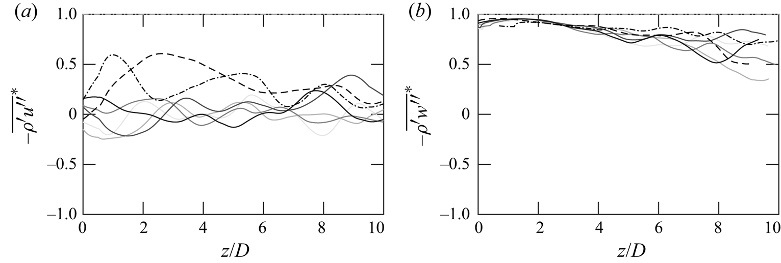
Figure 23. Centreline distributions of $\overline {\rho ' u''}^*$ (${=}\overline {\rho ' u''}/(\sqrt {\overline {\rho '^2}}\sqrt {{\widetilde {u^{''2}}}^{\vphantom{a^a}}})$ and $\overline {\rho ' w''}^*$ (${=}\overline {\rho ' w''}/(\sqrt {\overline {\rho '^2}}\sqrt {{\widetilde {w^{''2}}}^{\vphantom{a^a}}})$).

The budget analyses of the Reynolds stress and thermodynamic variances have shown that multiple mechanisms control the spatial development of density and the Reynolds stresses. To understand the mechanisms involved in the correlations of these two variables, the budget terms of turbulent mass fluxes are computed

(5.1)\begin{equation} \dfrac{\partial\widetilde{u_j}\overline{\rho' u''_i}}{\partial x_j} = B_{\rho}+\mathcal{P}_{\rho u}+P_{\rho u}+\varPi_{\rho u}+\varPhi_{\rho}+\epsilon_{\rho u}+\mathcal{T}_{\rho u}. \end{equation}

The turbulent mass-flux equation is governed by similar processes as the Reynolds stress equation. The term on the left-hand side is the convection term and it represents the spatial variation of the density and velocity correlation. The convection term is balanced by the terms on the right-hand side. These terms include the buoyancy $B_{\rho }$, production $\mathcal {P}_{\rho u}$ and $P_{\rho u}$, dilatation $\varPi _{\rho u}$, pressure distribution $\varPhi _{\rho u}$, dissipation $\epsilon _{\rho u}$ and transport $\mathcal {T}_{\rho u}$. The mathematical form of those terms is given as

(5.2a)\begin{gather} B_{\rho}={-}\dfrac{\overline{\rho'^2}}{\bar{\rho}}g_i \end{gather}

(5.2b)\begin{gather}\mathcal{P}_{\rho u}=\overline{\rho' u''_j}\dfrac{\partial\widetilde{u_i}}{\partial x_j} +\dfrac{\overline{\rho'^2}}{\bar{\rho}}\dfrac{\partial\overline{\sigma_{ij}}}{\partial x_j} \end{gather}

(5.2c)\begin{gather}P_{\rho u}={-}R_{ij}\dfrac{\partial\bar{\rho}}{\partial x_j} \end{gather}

(5.2d)\begin{gather}\varPi_{\rho u}={-}\bar{\rho}\overline{u''_i\dfrac{\partial u''_j}{\partial x_j}} \end{gather}

(5.2e)\begin{gather}\varPhi_{\rho}=\dfrac{1}{\bar{\rho}}\overline{p'\dfrac{\partial\rho'}{\partial x_i}} \end{gather}

(5.2f)\begin{gather}\epsilon_{\rho u}={-}\dfrac{1}{\bar{\rho}}\overline{\sigma'_{ij}\dfrac{\partial\rho'}{\partial x_j}} \end{gather}

(5.2g)\begin{gather}\mathcal{T}_{\rho u}={-}\dfrac{1}{\bar{\rho}}\overline{\dfrac{\partial\rho'p'}{\partial x_i}} +\dfrac{1}{\bar{\rho}}\overline{\dfrac{\partial\rho'\sigma'_{ij}}{\partial x_j}} -\dfrac{1}{\bar{\rho}}\dfrac{\partial}{\partial x_j}\dfrac{\overline{\rho' u''_iu''_j}}{\bar{\rho}}. \end{gather}

The budget terms of $\overline {\rho ' w''}$ are plotted in figure 24(a). The dominant terms in the evolution of $\overline {\rho ' w''}$ are $P_{\rho u}$ and $\varPi _{\rho u}$. This is consistent with the budget analysis of $\overline {\rho '^2}$ in which axial dilatation and the density gradient are the main mechanisms. However, dilatational effects become negative and production becomes positive to the mass-flux transport. During the initial plume development stage, $\varPi _{\rho u}$ has a monotonic increase. As the flow enters the mixing stage, $\varPi _{\rho u}$ starts decreasing. The decomposition of $\varPi _{\rho u}$ is shown in figure 24(b), in which the term is decomposed into horizontal and vertical components. The two components show opposite signs throughout the plumes. Unlike the main mechanisms in velocity and density, the dominant terms in $\overline {\rho ' w''}$ peak at $z/D\approx 5$ where $R_{33,max}$ occurs.

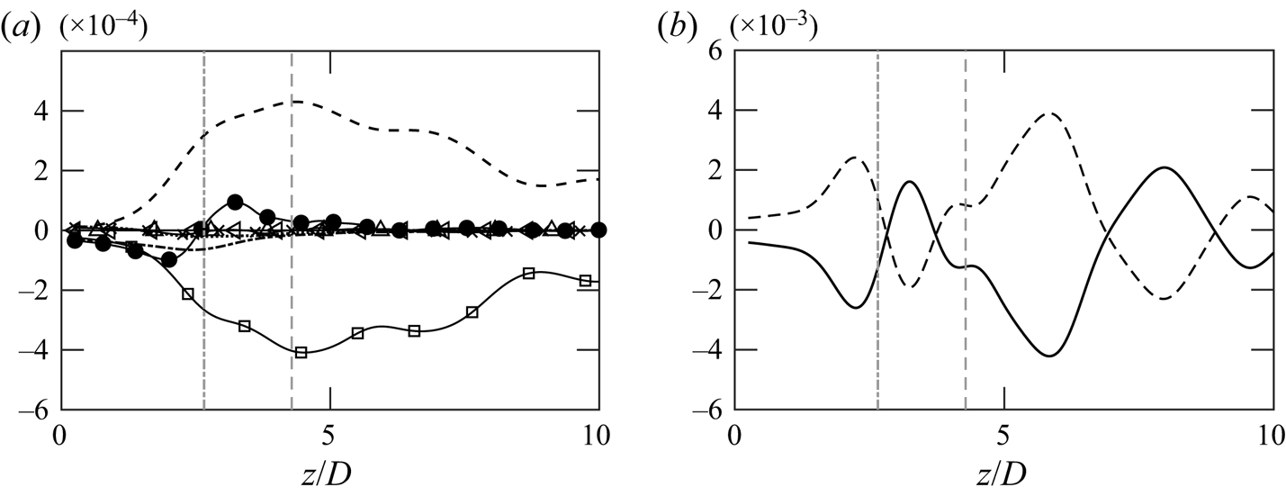
Figure 24. (a) Distributions of $\overline {\rho 'u''_3}$ budget terms from case 5: convection ($\bullet$); $B_{\rho }$ ($-{\cdot }$); $\mathcal {P}_{\rho u}$ ($\cdots$); $P_{\rho u}$ ($--$); $\varPi _{\rho u}$ ($\square$); $\varPhi _{\rho }$ ($\triangleleft$); $\epsilon _{\rho u}$ ($\Delta$); $\mathcal {T}_{\rho u}$ ($\times$). (b) Distributions of vertical ($-$) and horizontal ($--$) components of $\varPi _{\rho u}$. Vertical grey lines: $\overline {\rho ' w''}_{max}$ (dash-dotted) and $R_{33,max}$ (dashed).

5.2. Turbulent heat fluxes

Besides the turbulent mass fluxes, the correlation between temperature and the velocities can be realized through turbulent heat fluxes. Figure 25(a,b) shows the distributions of $\widetilde {T''u''}$ and $\widetilde {T''w''}$ normalized by the corresponding root-mean-square temperature and velocities. Similar to horizontal mass fluxes, a very weak connection can be seen between temperature and horizontal velocities in thermal plumes as the horizontal heat fluctuates around zero. A minor correlation exists in the plumes with methane and sulphur dioxide. In contrast, the correlations of temperature and the vertical velocities show a perfect anti-correlation near the source and slowly decrease as the plume rises. Similar to density, the turbulent heat fluxes show that temperature fluctuations are strongly associated with the axial motions.

Figure 25. Centreline distributions of $\widetilde {T'' u''}^*$ (${=}\widetilde {T'' u''}/(\sqrt {{\widetilde {T''^2}}^{\vphantom{a^a}}}\sqrt {{\widetilde {u^{''2}}}^{\vphantom{a^a}}})$ and $\widetilde {T'' w''}^*$ (${=}\widetilde {T'' w''}/(\sqrt {{\widetilde {T''^2}}^{\vphantom{a^a}}}\sqrt {{\widetilde {w^{''2}}}^{\vphantom{a^a}}})$).

As the correlation between temperature and the velocities exists, it is necessary to identify the mechanisms that control the correlations. The budget terms of the turbulent heat fluxes are computed

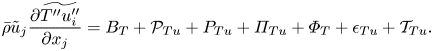(5.3)\begin{equation} \bar{\rho}\tilde{u}_j\dfrac{\partial\widetilde{T'' u''_i}}{\partial x_j} = B_T+\mathcal{P}_{Tu}+P_{Tu}+\varPi_{Tu}+\varPhi_{T}+\epsilon_{Tu}+\mathcal{T}_{Tu}. \end{equation}

Similar to the mass fluxes, the spatial development of turbulent heat flux is controlled by a balance of the terms on the right. The first three terms on the right are the productions due to buoyancy ($B_T$), mean flows ($\mathcal {P}_{Tu}$) and the temperature gradient ($P_{Tu}$). The following two terms are contributions from dilatation ($\varPi _{Tu}$) and pressure distribution ($\varPhi _{Tu}$). Finally, the last two terms are dissipation ($\epsilon _{Tu}$) and transport ($\mathcal {T}_{Tu}$). The explicit form of each term is given as follows:

(5.4a)\begin{gather} B_T={-}\overline{\rho' T''}g_i \end{gather}

(5.4b)\begin{gather}\mathcal{P}_{Tu}={-}\bar{\rho}\widetilde{T'' u''_j}\dfrac{\partial\tilde{u}_i}{\partial x_j}-\dfrac{1}{C_v}\overline{pu''_i}\dfrac{\partial\tilde{u}_j}{\partial x_j}+\dfrac{1}{C_v}\overline{\sigma_{jk}u''_i}\dfrac{\partial\tilde{u}_j}{\partial x_k} \end{gather}

(5.4c)\begin{gather}P_{Tu}={-}\bar{\rho} R_{ij}\dfrac{\partial \tilde{T}}{\partial x_j} \end{gather}

(5.4d)\begin{gather}\varPi_{Tu}={-}\dfrac{1}{C_v}\overline{pu''_i\dfrac{\partial u''_j}{\partial x_j}} \end{gather}

(5.4e)\begin{gather}\varPhi_{T}=\overline{p'\dfrac{\partial T''}{\partial x_i}} \end{gather}

(5.4f)\begin{gather}\epsilon_{Tu}=\dfrac{1}{C_v}\overline{\sigma_{jk}u''_i\dfrac{\partial u''_j}{\partial x_k}}-\overline{\sigma_{ij}\dfrac{\partial T''}{\partial x_j}} -\dfrac{1}{C_v}\overline{k_T\dfrac{\partial u''_i}{\partial x_j}\dfrac{\partial T}{\partial x_j}} \end{gather}

(5.4g)\begin{gather}\mathcal{T}_{Tu}={-}\dfrac{\partial\overline{\rho T'' u''_j u''_i}}{\partial x_j} -\dfrac{\partial\overline{p' T''}}{\partial x_i} +\dfrac{\partial\overline{\sigma_{ij}T''}}{\partial x_j} +\dfrac{1}{C_v}\dfrac{\partial}{\partial x_j}\overline{k_Tu''_i\dfrac{\partial T}{\partial x_j}}. \end{gather}

Here, $\epsilon$ contains both viscous and thermal dissipation and $\mathcal {T}_{Tu}$ includes turbulent, pressure, viscous and thermal transport.

The budget terms of turbulent heat fluxes are plotted in figure 26(a). The figure shows that the dominant terms for axial heat fluxes are the production of mean flow and dilatational motions. Similar to $\overline {\rho ' w''}$, both the dominant terms of $\widetilde {T'' w''}$ have a monotonic increase in the initial stage and peak at $R_{33,max}$. As the plume enters the mixing stage, the two mechanisms slowly decrease. The dilatation can be further decomposed into vertical and horizontal motions. Figure 26(b) shows that the two components have opposite distributions and counteract each other. In contrast to Reynolds stresses and thermodynamic variances, both the dilatational effects of $\overline {\rho ' w''}$ and $\widetilde {T'' w''}$ reach their maximum near $z/D=5$ at which the anisotropic phenomenon is weak. This observation seems to suggest that $\varPi _{\rho u}$ and $\varPi _{Tu}$ have a strong dependence on $w''$ rather than on the density. More details will be presented in the following discussion. Besides the production and dilatation, the pressure distribution and pressure transport (from figure 26c) are also important. Unlike $\overline {\rho '^2}$, $\widetilde {T''^2}$ and $\overline {\rho ' w''}$ which are only dependent on production and dilatation, the additional terms involved in the transport of $\widetilde {T'' w''}$ indicate a more complicated correlation between temperature and velocity. Further investigations will be conducted in future work.

Figure 26. (a) Distributions of $\widetilde {T'' w''}$ budget terms from case 5: convection ($\bullet$), $B_T$ ($-{\cdot }$); $\mathcal {P}_{Tu}$ ($\cdots$); $P_{Tu}$ ($--$); $\varPi _{Tu}$ ($\square$); $\varPhi _{T}$ ($\triangleleft$); $\epsilon _{Tu}$ ($\Delta$); $\mathcal {T}_{Tu}$ ($\times$). (b) Distributions of vertical ($-$) and horizontal ($--$) components of $\varPi _{Tu}$. (c) Distributions of transport terms: $\partial _z\overline {\rho T '' w^{''2}}$ ($-$); $\partial _z\overline {p' T''}$ ($--$); $\partial _z\overline {\sigma _{33}T''}$ ($-{\cdot }$); $\partial _z\overline {k_T w^{''2}\partial _zT}$ ($\cdots$). Vertical grey lines: $\widetilde {T''w''}_{max}$ (dash-dotted) and $R_{33,max}$ (dashed).

Finally, we present the budget terms of $\overline {\rho 'w''}$ and $\widetilde {T''w''}$ at $z/D=5$ where the variables peak in figure 27. Consistent with the centreline distributions, the radial transport of $\overline {\rho 'w''}$ is still dominated by $P_{\rho u}$ and $\varPi _{\rho u}$. For $\widetilde {T''w''}$, the main terms are $P_{Tu}$, $\varPi _{Tu}$, $\varPhi _T$ and $\mathcal {T}_{Tu}$. Despite the distance from the source, the figure shows that turbulent motions mostly occur within $x/D<0.5$.

Figure 27. (a) Radial profiles of $\overline {\rho 'w''}$ budgets at $z/D\approx 5$: $\partial _j(\widetilde {u_j}\overline {\rho 'w''})$ ($\bullet$); $P_{\rho u}$ ($--$) and $\varPi _{\rho u}$ ($\square$). (b) Radial profiles of $\widetilde {T''w''}$ budgets at the same heights: $\bar {\rho }\widetilde {u_j}\partial _j\widetilde {T''w''}$ ($\bullet$); $P_{Tu}$ (lines), $\varPi _{Tu}$ ($\square$), $\varPhi _{T}$ ($\triangleleft$) and $\mathcal {T}_{Tu}$ ($\times )$.

5.3. Spectra and characteristic scales

Turbulent fluctuations exist in a wide range of scales. As the axial dilatation is identified as being the mechanism that contributes to thermodynamic fluctuations in the buoyant plumes, it is important to identity the scales at which the interaction occurs. We plot the spectra of the axial mass and heat fluxes in figure 28(a,b). The spectra are compared at multiple different heights. The figure shows that the thermodynamic variables are correlated with velocity at large scales. In addition, the spectra of the correlation resemble the energy spectra of vertical velocity. The buoyancy range with $-3$ slope is observed in both fluxes at different heights. The observed $-3$, instead of $-2.7$, slope confirms that the velocities are dominant over the thermodynamic fluctuations in the correlation term. The similarity between $E_{ww}$, $E_{\rho w}$ and $E_{Tw}$ indicates that the correlation is influenced by velocity fluctuations rather than the thermodynamic variables.

Figure 28. Spectra of (a) $\rho u$ and (b) $Tw$ from thermal plume at $z\approx 2D$ (solid), $z\approx 3D$ (dashed), $z\approx 5D$ (dash-dotted) and $z\approx 10D$ (dotted). Same colours and lines as figure 19.

The present work has shown that vertical velocity strongly correlates with density and temperature. From the spectra, we realize that these correlations are mostly influenced by velocity fluctuations. To further understand the related temporal characteristics, we present the characteristic time scales (Skamarock et al. Reference Skamarock, Park, Klemp and Snyder2014)

(5.5)\begin{equation} \tau=k^{{-}3/2}E(k)^{{-}1/2} \end{equation}

in figure 29. From (5.5), $\tau (k)$ represents the characteristic time in synoptic scale, which corresponds to the buoyancy range. The characteristic time scale of vertical velocity, $\tau _w$, reaches an asymptotic state in the buoyancy regime and such an observation is consistent with other studies (Skamarock et al. Reference Skamarock, Park, Klemp and Snyder2014). Further, this asymptotic condition is invariant with plume height. On the other hand, although the time scales for density and temperature also asymptote at higher wavenumbers, the asymptotic value increases with increasing plume height. The comparison of the time scales $\tau _w$, $\tau _{\rho }$ and $\tau _T$ suggest that the turnover time scales of velocity are much smaller than the thermodynamic variables.

Figure 29. Characteristic time scales from the spectra of (a) vertical velocity ($w''$), (b) density ($\rho '$) and (c) temperature ($T''$) at $z/D\approx 2$ (solid), $z/D\approx 3$ (dashed), $z/D\approx 5$ (dash-dotted) and $z/D\approx 10$ (dotted).

The present study focused on the mechanisms for the evolution of Reynolds stresses and thermodynamic fluctuations for active scalar mixing. The thermodynamic fluctuations are attributed to the axial dilatation at large scales. In isotropic turbulence, thermodynamic spectra mostly show a spectral slope $\approx -7/3$ at the intermediate scales. On the contrary, such a slope is not found in the present work. The thermodynamic spectra show a value of $-2.7$, which is similar with the studies of stratified turbulence (Carnevale et al. Reference Carnevale, Briscolini and Orlandi2001; Waite Reference Waite2011). Since buoyancy was found to be negligible in the cross-relations of velocity and thermodynamic variables, the change of spectral slope from isotropic turbulence is an interesting and important discovery.