


1. Introduction
Double-diffusive convection represents a mixing process driven by two fluid components that diffuse at different rates. It is of great significance in oceanography, geophysics, astrophysics and engineering (e.g. Turner Reference Turner1985; Schmitt Reference Schmitt1994; Radko Reference Radko2013; Garaud Reference Garaud2018). Regarding the double-diffusive convection in oceanography, the temperature field constitutes the faster diffuser while the salinity field the slower diffuser (Schmitt Reference Schmitt1994). Away from the freezing point, the density of water is a decreasing function of temperature but an increasing function of salinity. In low-latitude regions, warm and salty waters are generally located above cold and fresh waters (Radko Reference Radko2013), which makes the (sub)tropical oceans susceptible to the well-known fingering convection, i.e. salt fingers. In contrast, seawater in polar regions is stratified such that both salinity and temperature decrease upward, thus prone to diffusive convection, viz. oscillatory double-diffusive convection (ODDC). The onset conditions for instability in double-diffusive convection have been well understood in classical cases (e.g. Veronis Reference Veronis1965; Baines & Gill Reference Baines and Gill1969; Balmforth et al. Reference Balmforth, Ghadge, Kettapun and Mandre2006). Generally, the linear instability of double-diffusive convection can take place in the form of either steady or oscillatory convection, depending on the detailed sets of parameters (Veronis Reference Veronis1965; Balmforth et al. Reference Balmforth, Ghadge, Kettapun and Mandre2006).
Over the past decades, sea ice in the Arctic Ocean has been observed to decrease at least by 40% in volume (Rothrock, Yu & Maykut Reference Rothrock, Yu and Maykut1999; Wadhams & Davis Reference Wadhams and Davis2000; Deser & Teng Reference Deser and Teng2008). Solar radiation and basal melting are the two main driving factors of the dramatic sea ice loss (e.g. Perovich et al. Reference Perovich, Richter-Menge, Polashenski, Elder, Arbetter and Brennick2014). Regarding the basal melting, the thermohaline stratification lying between the cold, fresh meltwater and the warm, saline Atlantic intruding water was quite stable in the past, so that the warm Atlantic intruding water, which carries enough heat to melt all the ice in the Arctic, cannot effectively transfer its heat to the lower surface of the ice (Turner Reference Turner2010). However, recent measurement of the Eurasian Basin has indicated that the Atlantic warm tongue is shoaling and the stability of the stratification layer is weakened, which allows more heat to penetrate through the halocline and enter in the lower surface of sea ice, thereby leading to the so-called ‘Atlantification’ of the Arctic Ocean (Polyakov et al. Reference Polyakov2017). In fact, basal melting plays an even more important role in the melting of the Antarctica ice shelves, which have lost more than 50% of their mass by the basal double-diffusive process (Rignot et al. Reference Rignot, Jacobs, Mouginot and Scheuchl2013; Begeman et al. Reference Begeman, Tulaczyk, Marsh, Mikucki, Stanton, Hodson, Siegfried, Powell, Christianson and King2018). As mentioned before, high-latitude oceans are generally stratified in the diffusive regime. For instance, a borehole oceanographic observation on the Ross Ice Shelf indicates that near the grounding zones, the value of the Turner angle, which is a common measure of the stratification pattern, is mainly within (−90°, −45°), thereby susceptible to diffusive convection (Begeman et al. Reference Begeman, Tulaczyk, Marsh, Mikucki, Stanton, Hodson, Siegfried, Powell, Christianson and King2018). So far, however, instability properties of the subglacial double-diffusive convection in various ocean conditions, e.g. buoyancy by double diffusion, ice melting and background current, have not been well understood. Specifically, while previous studies have demonstrated the non-trivial effect of a solid–liquid phase boundary on the stability of Rayleigh–Bénard convection (Davis, Müller & Dietsche Reference Davis, Müller and Dietsche1984; Kim, Lee & Choi Reference Kim, Lee and Choi2008; Vasil & Proctor Reference Vasil and Proctor2011; Toppaladoddi & Wettlaufer Reference Toppaladoddi and Wettlaufer2019), this effect has not been examined in a subglacial diffusive convection system. In addition, despite of the systematic examination of the combined effects of the shear and double diffusion (i.e. the thermohaline-shear instability) from the perspective of asymptotic stability analysis and direct numerical simulation (DNS) (Radko Reference Radko2016; Brown & Radko Reference Brown and Radko2019; Radko Reference Radko2019), the transient behaviour and the nature (i.e. oscillatory, steady and dynamic) of this newly found instability are still left to be resolved. These two points are reviewed individually below.
Regarding the effects of melting/freezing on the buoyancy-driven instability, let us first have a look at the results of investigations on single-component cases (that is, with the heat transport only). Davis et al. (Reference Davis, Müller and Dietsche1984) have studied the bifurcation and pattern formation of single-component buoyancy-driven convection underneath a steady solid–liquid interface. They considered a steady base state by assuming that the heat entering and leaving the interface balances each other. It is found that at the onset of flow motion, the solid–liquid interface behaves like a planar rigid solid of imperfect thermal conductivity. With the increase of solid depth, the conductivity effectively decreases so that the critical Rayleigh number Rac and critical wavenumber kc both decrease. For sufficiently large solid thickness, (Rac, kc) asymptote to (1493, 2.815). Recently, this work has been extended by Toppaladoddi & Wettlaufer (Reference Toppaladoddi and Wettlaufer2019) to study the effect of low-Péclet-number Couette flow. It is found that the imposed shear tends to stabilize the system by inhibiting the vertical heat flux. Vasil & Proctor (Reference Vasil and Proctor2011) studied the instability of Rayleigh–Bénard convection subject to a different solid–liquid interface. They considered a Stefan system with an isothermal solid, in which the liquid layer will slowly deepen as time progresses. At the large-Stefan-number limit in which the melting is very slow, the phase interface acts as a fixed-flux boundary, which results in the convection threshold decreasing from (1707.763, 3.116) (Chandrasekhar Reference Chandrasekhar1961) to (1295.78, 2.552). The decrease of convection threshold due to the phase boundary has also been observed by Kim et al. (Reference Kim, Lee and Choi2008) in a fast-melting system.
In two-component cases, few attempts have been made to study the double-diffusive instability in the presence of an ice–water interface. In places such as Greenland (e.g. McDougall Reference McDougall1983; McPhee Reference McPhee2008; Chandler et al. Reference Chandler2013) and the Arctic (e.g. Polashenski, Perovich & Courville Reference Polashenski, Perovich and Courville2012; Polashenski et al. Reference Polashenski, Golden, Perovich, Skyllingstad, Arnsten, Stwertka and Wright2017), strong solar radiation in summer is able to cause the seasonal melting/freezing at the surface of ice shelves. Martin & Kauffman (Reference Martin and Kauffman1974) studied the dynamics of under-ice melt ponds resulting from the aforementioned process. They focused on the ice growth (the so-called false bottom) in the system, which was found to go through three different stages: nucleation, lateral growth and upward migration due to the temperature and salinity gradient. The formation of a false bottom is closely correlated with the double diffusion. Recently, Hirata, Goyeau & Gobin (Reference Hirata, Goyeau and Gobin2012) investigated the onset of double-diffusive convection in the under-ice melt ponds. They considered the water density inversion and showed that the depth of the ice matrix plays a key role in the stability of the under-ice melt layer. Particularly, increasing the depth of the ice layer will decrease the convection threshold, which is consistent with the single-component cases (Davis et al. Reference Davis, Müller and Dietsche1984; Toppaladoddi & Wettlaufer Reference Toppaladoddi and Wettlaufer2019). However, the depth of the melt layer has a marginal influence, due to the compensation between stabilizing salinity gradient and destabilizing temperature gradient which simultaneously change when increasing the liquid depth.
Regarding the effect of background current on double-diffusive instability, much attention has been paid to salt fingers in the early stage. Linden (Reference Linden1974) studied the effect of a steady Couette flow on fingering convection between two planes. Results showed that the shear affects the fingering instability in a way similar to thermally stratified shear flow. For instance, longitudinal rolls are the preferred mode and unaffected by the shear. In addition, the instabilities of both transverse and oblique rolls tend to be inhibited by the shear since the mean flow can absorb energy from the spanwise perturbations. Recently, Konopliv, Lesshafft & Meiburg (Reference Konopliv, Lesshafft and Meiburg2018) performed a transient growth analysis of a similar problem. Their results showed that even though the Couette flow is vertically unbounded, it can also damp the fingering instability. Most importantly, they detected the transient growth of fingering convection which exists regardless of whether there is a shear or not. This transient growth is attributed to a mechanism relying on the density stratification, different from the Orr mechanism or lift-up mechanism which relies on shear (Jerome, Chomaz & Huerre Reference Jerome, Chomaz and Huerre2012). It should be noted that Linden (Reference Linden1974) and Konopliv et al. (Reference Konopliv, Lesshafft and Meiburg2018) were not concerned with the shear-driven instability in their studies. In fact, the basic shear itself may yield dynamic instability such as Kelvin–Helmholtz instability, which can interact with double-diffusive stratification and thus lead to the formation of thermohaline staircases (Symth & Kimura Reference Symth and Kimura2007). Radko & Stern (Reference Radko and Stern2011) studied the fingering instability in the presence of a shear with sinusoidal velocity profile (namely the Kolmogorov flow). By assuming triply periodic boundary conditions, they identified two kinds of instability that dominate the system. For small values of Richardson number Ri, the classical Kelvin–Helmholtz instability is the fastest growing mode; for large values of Ri, however, the Kelvin–Helmholtz instability will be superseded by the thermohaline-shear instability, a newly found oscillatory instability that bears strong resemblance to the collective instability observed in thermally stratified Kolmogorov flow (Balmforth & Young Reference Balmforth and Young2002).
Recently, to understand the thermohaline layering of diffusively stable oceans in high-latitude regions, Radko (Reference Radko2016) investigated the diffusive instability in the presence of the Kolmogorov flow. Both results of DNS and linear stability analysis indicated that the interaction between the shear and density stratification can surprisingly destabilize the system that is individually stable to Kelvin–Helmholtz and diffusive instabilities. It is clear that as with Kelvin–Helmholtz instability, the fastest growing mode in the thermohaline-shear instability is the transverse rolls, which is in contrast to the fingering cases (Linden Reference Linden1974; Symth & Kimura Reference Symth and Kimura2007; Radko & Stern Reference Radko and Stern2011; Konopliv et al. Reference Konopliv, Lesshafft and Meiburg2018). Radko (Reference Radko2016) performed an energy analysis to suggest that there exist two regimes of the energy balance of thermohaline-shear instability. Different from the low-Pe regime (Pe is the Péclet number) in which the energy production by shear is negligible compared with that by temperature gradient, the dominant energy balance in the high-Pe regime is between the energy produced by shear and dissipated by viscosity. It is noted that in this seminal work, there are three questions remaining to be resolved, which partially motivates us to further study the sheared diffusive convection by analysing the energy budgets with the help of non-modal analysis.
First, in the high-Pe regime, the author attributed the main energy source of amplifying the disturbance to the unstable temperature gradient, which is definitely true in the low-Pe regime only. This might be because in the energy analysis, the author fixed all controlling parameters except Pe, which leads to the overestimation of energy contribution of heat diffusion (especially in the high-Pe regime). Note that in the thermohaline-shear instability, the critical temperature gradient is varied when varying Pe (specifically, we will show that in fact the critical Rayleigh number is a rapidly decreasing function of Pe).
Second, Radko (Reference Radko2016) rationalized the catalytic role of shear in the energy transfer from the density gradient to the perturbed hydrodynamic field by hypothesizing that the existence of a shear increases the residual energy gain of a particle in an oscillation cycle. However, this hypothesis requires that the thermohaline-shear instability is within the oscillatory rather than steady instability regime, which will be addressed in this work.
Finally, the analysis of Radko (Reference Radko2016) focused only on the asymptotic growth of the perturbation, while as mentioned before, it has been confirmed by Konopliv et al. (Reference Konopliv, Lesshafft and Meiburg2018) that the initial transient growth can occur in double-diffusive convection even in the absence of a shear. Considering that the short-term disturbance behaviour can sometimes overdraw the long-term one determined by the eigenvalue analysis (Schmid & Henningson Reference Schmid and Henningson2001), it is necessary to inspect the initial transient growth of thermohaline-shear instability.
Nevertheless, as a plausible mechanism of the generation of staircases in the Arctic, thermohaline-shear instability has been discussed by Garaud (Reference Garaud2017) in wider geophysical prospects and also studied numerically with a linear velocity profile (Yang et al. Reference Yang, Verzicco, Lohse and Caufield2022). In addition, to consider the effects of internal gravity waves, this instability has been investigated in the case of shear with time-dependent magnitude (Brown & Radko Reference Brown and Radko2019; Radko Reference Radko2019). Specifically, a temporal record of the quadratic perturbation norm (not the non-modal analysis) by Radko (Reference Radko2019) indicated that the overall exponential growth is modulated by small-scale oscillations. Since the small-scale oscillations acquire the angular frequency twice of the time-dependent mean shear, it is believed that this oscillatory behaviour is inherited from the base flow so that it cannot help to identify whether the thermohaline-shear instability is oscillatory or steady.
As shown above, few works have studied the effects of an ice–water interface on the linear instability of diffusive convection. However, previous studies of effects of shear on diffusive instability focused mainly on the thermohaline-shear instability, so a more comprehensive investigation in this regard is necessary. As for the thermohaline-shear instability, there are still several essential problems left to be resolved. This leads to the aims of the present study: (i) investigate the diffusive instability in the presence of an ice–water interface; (ii) study the transition from oscillatory to steady, and to dynamic instability; and (iii) examine the transient growth of diffusive convection in the absence/presence of shear. To this end, in addition to the modal stability analysis, non-modal stability analysis and energy analysis are also adopted to improve our understanding of the problems. This paper is organized as follows. In § 2, we formulate the problem. In § 3, we derive the linearized equations and provide a systematic code validation. The results are present in § 4 and conclusions are drawn in § 5.
2. Problem formulation
This work extends on that of Toppaladoddi & Wettlaufer (Reference Toppaladoddi and Wettlaufer2019) to account for salinity stratification. As sketched in figure 1, we consider an idealized system which consists of an infinite horizontal liquid layer of thickness h 0 sandwiched between a lower fixed plane and an upper solid layer. The upper solid layer corresponds to the ice shelf of thickness d 0. A Cartesian coordinate system (x, y, z) is centred on the bottom of the channel with the y-axis pointing vertically upwards. The base of the water is held at the temperature Tb higher than that at the upper surface of ice shelf Tu. The melting/freezing temperature of ice, i.e. Ti, is such that Tu < Ti < Tb, which allows the phase interface to move upwards or downwards, depending on the heat fluxes towards and away from the interface. When the heat flux across the liquid layer is larger than those across the ice layer, the system undergoes melting, which produces fresh water near the ice–ocean interface so that the ambient salinity is stratified as with the temperature in the liquid. The configuration considered here, that both the temperature and salinity are increasing functions of the water depth, is based on the observations of Begeman et al. (Reference Begeman, Tulaczyk, Marsh, Mikucki, Stanton, Hodson, Siegfried, Powell, Christianson and King2018). The salinities of lower and upper surfaces of the liquid layer are denoted by Sb and Si. Following Hewitt (Reference Hewitt2020), we assume the ice void of salinity for convenience. In addition, as with Radko (Reference Radko2016), we impose a Kolmogorov flow in the liquid layer to model the effect of ambient current, with U 0 being the maximum of the velocity profile.

Figure 1. Schematic description of the problem.
2.1 Governing equations
In the liquid, the governing equations for sheared double-diffusive process are (e.g. Radko Reference Radko2013)
 \begin{gather}\boldsymbol{\nabla }\boldsymbol{\cdot }\boldsymbol{U} = 0,\end{gather}
 \begin{gather}\frac{{\partial \boldsymbol{U}}}{{\partial t}} + \boldsymbol{U}\boldsymbol{\cdot }\boldsymbol{\nabla U} =- \frac{{\boldsymbol{\nabla }P}}{{{\rho _0}}} + \upsilon {\nabla ^2}\boldsymbol{U} + g\frac{{\rho - {\rho _0}}}{{{\rho _0}}}\boldsymbol{y},\end{gather}
 \begin{gather}\frac{{\partial T}}{{\partial t}} + \boldsymbol{U}\boldsymbol{\cdot }\boldsymbol{\nabla }T = {k_T}{\nabla ^2}T,\end{gather}
 \begin{gather}\frac{{\partial S}}{{\partial t}} + \boldsymbol{U}\boldsymbol{\cdot }\boldsymbol{\nabla }S = {k_S}{\nabla ^2}S,\end{gather}
where U = (U, V, W) is the velocity field, P the dynamic pressure, g the acceleration due to gravity, ρ (ρ 0) the (reference) density, υ the kinematic viscosity and y the unit vector in the y direction. Here, (T, S) represent the temperature and salinity, with their molecular diffusivities denoted by (kT, kS). We assume the linear equation of state for simplicity (Radko Reference Radko2013):
 \begin{equation}\rho = {\rho _0}[1 + {\alpha _S}(S - {S_0}) - {\alpha _T}(T - {T_0})],\end{equation}
where (αT, αS) are the constant expansion/contraction coefficients, and (T 0, S 0) are the reference temperature and salinity.
The heat transport in the solid is governed by thermal diffusion, viz.
 \begin{equation}\frac{{\partial {T_s}}}{{\partial t}} = {k_T}{\nabla ^2}{T_s},\end{equation}
where Ts is the temperature in the solid. Note that the thermal diffusivities in the solid and the liquid are identical for simplicity.
The ice–water interface is at the temperature of melting/freezing, and its evolution is governed by the Stefan condition, i.e.
 \begin{equation}T = {T_s} = {T_i},\quad {\rho _0}L\frac{{\partial h}}{{\partial t}} = \boldsymbol{n}\boldsymbol{\cdot }\kappa (\nabla {T_s} - \nabla T),\end{equation}
where L is the latent heat of fusion, h = h(x, z) the height of the interface, n the unit vector normal to the interface and κ the thermal conductivity.
In addition to the Stefan condition, the remaining boundary conditions are
 \begin{gather}\boldsymbol{U} = {\textbf{0}},\quad T = {T_b},\quad S = {S_b}\quad \textrm{at}\;y = 0,\end{gather}
 \begin{gather}\boldsymbol{U} = {\textbf{0}},\quad S = {S_i}\quad \textrm{for}\;y = {h_0},\end{gather}
 \begin{gather}{T_s} = {T_u}\quad {\rm at}\;y = {h_0} + {d_0}.\end{gather}
To place the above formulations in dimensionless form, we introduce the following scales:
 \begin{equation}\left. {\begin{array}{*{20}{c@{}}} {x,y,z \sim {h_0},\quad u,v,w \sim {U_0},\quad t \sim \dfrac{{{h_0}}}{{{U_0}}},}\\ {T - {T_0} \sim \varDelta T = {T_b} - {T_i},\quad S - {S_0} \sim \varDelta S = {S_b} - {S_i},\quad P \sim \rho U_0^2.} \end{array}} \right\}\end{equation}
Here we have T 0 = Ti. These scalings give rise to the following dimensionless numbers, viz.
 \begin{equation}\left. {\begin{array}{*{20}{c@{}}} {Ra = \dfrac{{g{\alpha_T}\varDelta Th_0^3}}{{\upsilon {k_T}}},\quad {R_S} = \dfrac{{g{\alpha_S}\varDelta Sh_0^3}}{{\upsilon {k_S}}},\quad Re = \dfrac{{{U_0}{h_0}}}{\upsilon },}\\ {Pr = \dfrac{\upsilon }{{{\alpha_T}}},\quad \beta = \dfrac{{{k_S}}}{{{k_T}}},\quad St = \dfrac{L}{{{c_p}\varDelta T}},\quad \varLambda = \dfrac{{{T_i} - {T_u}}}{{\varDelta T}}.} \end{array}} \right\}\end{equation}
Here, Ra and RS are the thermal and the salinity Rayleigh numbers which measure the buoyancy due to temperature and salinity gradients, respectively. The Reynolds number Re represents the strength of the shear flow. The Prandtl number Pr compares kinematic viscosity to thermal diffusivity. Additionally, β is the diffusivity ratio of salt and heat. Since we are concerned here with the diffusive convection of high-latitude oceans, we will consider Pr and β to be fixed at Pr = 10 and β = 0.01 throughout all calculations, unless otherwise specified. The Stefan number St denotes the ratio between the latent heat and specific heat (cp), and  $\varLambda$ is the ratio of the temperature differences across the liquid and the ice layers. Maintaining the pre-scaled notation, the governing equations become
 \begin{gather}\boldsymbol{\nabla }\boldsymbol{\cdot }\boldsymbol{U} = 0,\end{gather}
 \begin{gather}\frac{{\partial \boldsymbol{U}}}{{\partial t}} + \boldsymbol{U}\boldsymbol{\cdot }\boldsymbol{\nabla U} =- \boldsymbol{\nabla }P + \frac{1}{{Re}}{\nabla ^2}\boldsymbol{U} + \frac{{Ra}}{{Pr \cdot R{e^2}}}\boldsymbol{\cdot }T\boldsymbol{\cdot }\boldsymbol{y} - \frac{{{R_S} \cdot \beta }}{{Pr \cdot R{e^2}}}\boldsymbol{\cdot }S\boldsymbol{\cdot }\boldsymbol{y},\end{gather}
 \begin{gather}\frac{{\partial T}}{{\partial t}} + \boldsymbol{U}\boldsymbol{\cdot }\boldsymbol{\nabla }T = \frac{1}{{Pr \cdot Re}}{\nabla ^2}T,\end{gather}
 \begin{gather}\frac{{\partial S}}{{\partial t}} + \boldsymbol{U}\boldsymbol{\cdot }\boldsymbol{\nabla }S = \frac{\beta }{{Pr \cdot Re}}{\nabla ^2}S,\end{gather}
 \begin{gather}\frac{{\partial {T_s}}}{{\partial t}} = \frac{1}{{Pr \cdot Re}}{\nabla ^2}{T_s},\end{gather}
with accompanying boundary conditions
 \begin{gather}\boldsymbol{U} = {\textbf{0}},\quad S = 1,\quad T = 1\quad \textrm{at}\;y = 0,\end{gather}
 \begin{gather}\boldsymbol{U} = {\textbf{0}},\quad S = \textrm{0},\quad T = {T_s} = 0,\quad St\frac{{\partial h}}{{\partial t}} = \boldsymbol{n}\boldsymbol{\cdot }(\boldsymbol{\nabla }{T_s} - \boldsymbol{\nabla }T),\quad \textrm{for}\;y = 1,\end{gather}
 \begin{gather}{T_s} =- \varLambda \quad \textrm{at}\;y = 1 + {d_0}.\end{gather}
3. Linear stability equations
In this section, we derive the stability equations for infinitesimal disturbances in the present system. We first focus on the dynamics in the liquid. Based on the linear stability theory (Schmid & Henningson Reference Schmid and Henningson2001), all variables are separated into the basic state and a departure from it, i.e.
 \begin{equation}\boldsymbol{U} = \bar{\boldsymbol{U}} + \boldsymbol{u},\quad P = \bar{P} + p,\quad T = \bar{T} + \theta ,\quad {T_s} = \overline {{T_s}} + {\theta _s},\quad S = \bar{S} + s,\end{equation}
where u = (u, v, w), p, θ, θs and s represent the velocity vector, pressure, temperature and salinity in the perturbed state, while  $\bar{\boldsymbol{U}}$, $\bar{P}$, $\bar{T}$, $\overline {{T_s}}$ and $\bar{S}$ are the corresponding base-state variables. Inserting the decompositions into (2.8a–d), subtracting the equation for the basic state and omitting the nonlinear terms, we obtain
 \begin{gather}\boldsymbol{\nabla }\boldsymbol{\cdot }\boldsymbol{u} = 0,\end{gather}
 \begin{gather}\frac{{\partial \boldsymbol{u}}}{{\partial t}} + (\boldsymbol{u}\boldsymbol{\cdot }\boldsymbol{\nabla })\bar{\boldsymbol{U}} + (\bar{\boldsymbol{U}}\boldsymbol{\cdot }\boldsymbol{\nabla })\boldsymbol{u} =- \boldsymbol{\nabla }p + \frac{1}{{Re}}{\nabla ^2}\boldsymbol{u} + \frac{{Ra}}{{R{e^2} \cdot Pr}}\boldsymbol{\cdot }\theta \boldsymbol{\cdot }\boldsymbol{y} - \frac{{{R_S} \cdot \beta }}{{R{e^2} \cdot Pr}}\boldsymbol{\cdot }s\boldsymbol{\cdot }\boldsymbol{y},\end{gather}
 \begin{gather}\frac{{\partial \theta }}{{\partial t}} + (\boldsymbol{u}\boldsymbol{\cdot }\boldsymbol{\nabla })\bar{T} + (\bar{\boldsymbol{U}}\boldsymbol{\cdot }\boldsymbol{\nabla })\theta = \frac{1}{{Re \cdot Pr}}{\nabla ^2}\theta ,\end{gather}
 \begin{gather}\frac{{\partial s}}{{\partial t}} + (\boldsymbol{u}\boldsymbol{\cdot }\boldsymbol{\nabla })\bar{S} + (\bar{\boldsymbol{U}}\boldsymbol{\cdot }\boldsymbol{\nabla })s = \frac{\beta }{{Re \cdot Pr}}{\nabla ^2}s.\end{gather}
The boundary conditions for the velocity and salinity fluctuations read (the Stefan condition will be discussed later)
 \begin{equation}\boldsymbol{u} = 0\quad \textrm{and}\quad s = 0\quad \textrm{for}\;y = 0\;\textrm{and}\;y = 1.\end{equation}
3.1 Base-state solutions
In this study, we consider a steady and horizontally homogeneous base state in which the ice–water interface is unmovable unless the vertical flow motion sets in. This steady state is reasonable due to the fact that, given that the solid is conducting, any melting process will eventually reach an equilibrium state, as long as the heat fluxes entering and leaving the interface balance (e.g. Purseed, Favier & Duchemin Reference Purseed, Favier and Duchemin2020). Therefore, in the base state, we have (Toppaladoddi & Wettlaufer Reference Toppaladoddi and Wettlaufer2019)
 \begin{equation}\frac{{\textrm{d}\bar{T}}}{{\textrm{d}y}} = \frac{{\textrm{d}\overline {{T_s}} }}{{\textrm{d}y}}\quad \textrm{at}\;y = 1.\end{equation}
This leads to
 \begin{equation}{d_0} = \varLambda ,\end{equation}
which indicates that the thicknesses of the liquid and solid layers in the equilibrium state are determined by the values of Tb, Ti and Tu (Davis et al. Reference Davis, Müller and Dietsche1984).
The base-state temperature profile is given by (Davis et al. Reference Davis, Müller and Dietsche1984; Toppaladoddi & Wettlaufer Reference Toppaladoddi and Wettlaufer2019)
 \begin{equation}\bar{T}(y) = 1 - y,\quad 0 \le y \le 1\quad \textrm{and}\quad \overline {{T_s}} (y) = 1 - y,\quad 1 \le y \le 1 + {d_0}.\end{equation}
Regarding the base state of salinity, we have
 \begin{equation}\bar{S}(y) = 1 - y,\quad 0 \le y \le 1.\end{equation}
For the base flow, we are mainly interested in the hydrostatic base state and Kolmogorov flow (Radko Reference Radko2016), which are respectively given by
 \begin{gather}\bar{\boldsymbol{U}}(y) = 0\quad \textrm{for}\;\textrm{hydrostatic}\;\textrm{state},\end{gather}
 \begin{gather}\bar{U}(y) =- \textrm{sin}(2{\rm \pi} y),\quad \bar{V} = \bar{W} = 0\quad \textrm{for}\;\textrm{Kolmogorov}\;\textrm{flow}\;\textrm{with}\;0 \le y \le 1.\end{gather}
3.2 Matrix representation
After the given base state is substituted in the linearized equations and the pressure term is eliminated from the obtained equations, the linearized system can be rewritten as
 \begin{gather}\begin{array}{ccccc} \dfrac{{\partial {\nabla ^2}v}}{{\partial t}} & = \left( { - \bar{U}\dfrac{\partial }{{\partial x}}{\nabla^2} + \dfrac{{{\textrm{d}^2}\bar{U}}}{{\textrm{d}{y^2}}}\dfrac{\partial }{{\partial x}} + \dfrac{1}{{Re}}{\nabla^4}} \right)v + \dfrac{{Ra}}{{R{e^2} \cdot Pr}}\left( {{\nabla^2} - \dfrac{{{\partial^2}}}{{\partial {y^2}}}} \right)\theta \\ & \quad - \dfrac{{{R_S} \cdot \beta }}{{R{e^2} \cdot Pr}}\left( {{\nabla^2} - \dfrac{{{\partial^2}}}{{\partial {y^2}}}} \right)s, \end{array}\end{gather}
 \begin{gather}\frac{{\partial \eta }}{{\partial t}} =- \frac{{\textrm{d}\bar{U}}}{{\textrm{d}y}}\frac{\partial }{{\partial z}}v + \left( { - \bar{U}\frac{\partial }{{\partial x}} + \frac{1}{{Re}}{\nabla^2}} \right)\eta ,\end{gather}
 \begin{gather}\frac{{\partial \theta }}{{\partial t}} =- \frac{{\textrm{d}\bar{T}}}{{\textrm{d}y}}v + \left( { - \bar{U}\frac{\partial }{{\partial x}} + \frac{1}{{Re \cdot Pr}}{\nabla^2}} \right)\theta ,\end{gather}
 \begin{gather}\frac{{\partial s}}{{\partial t}} =- \frac{{\textrm{d}\bar{S}}}{{\textrm{d}y}}v + \left( { - \bar{U}\frac{\partial }{{\partial x}} + \frac{\beta }{{Re \cdot Pr}}{\nabla^2}} \right)s,\end{gather}
where η is the vorticity in the y-direction, defined by
 \begin{equation}\eta = \frac{{\partial u}}{{\partial z}} - \frac{{\partial w}}{{\partial x}}.\end{equation}
For clarity, the linearized system (3.7) can be recast in matrix notation, viz.
 \begin{equation}\boldsymbol{\mathsf{A}}\frac{{\partial \boldsymbol{\zeta }}}{{\partial t}} = \boldsymbol{\mathsf{B}}\zeta \quad \Rightarrow \quad \frac{{\partial \boldsymbol{\zeta }}}{{\partial t}} = \boldsymbol{\mathsf{L}}\zeta ,\end{equation}
where ζ = (v, η, θ, s)T and  $\boldsymbol{\mathsf{L}}$ = $\boldsymbol{\mathsf{A}}$−1 $\boldsymbol{\mathsf{B}}$ is the linearized Navier–Stokes operator.
We seek solutions of (3.9) in the following wave-like form:
 \begin{equation}f(x,y,z,t) = {f^\ast }(y)\ \textrm{exp}(\textrm{i}kx + \textrm{i}mz - \textrm{i}\omega t),\end{equation}
where f corresponds to (v, η, θ, s), f* = (v*, η*, θ*, s*) is the shape function, k and m the streamwise and spanwise wavenumbers, and ω the circular frequency of the perturbation. Note that ω is complex valued, with the real part ωr being the phase speed while the imaginary part ωi the growth rate. Substituting (3.10) into (3.9), we arrive at an eigenvalue problem,
 \begin{equation}- \textrm{i}\omega {\boldsymbol{\zeta }^\ast } = \boldsymbol{\mathsf{L}}{\boldsymbol{\zeta }^\ast },\end{equation}
where ζ* is the eigenvector of the eigenvalue −iω.
The boundary conditions for the amplitudes of the perturbed velocity, vorticity and salinity are
 \begin{equation}{v^\ast } = \frac{{\partial {v^\ast }}}{{\partial y}} = {\eta ^\ast } = {s^\ast } = 0\quad \textrm{for}\;y = 0\;\textrm{and}\;y = 1.\end{equation}
The boundary condition for the perturbed temperature at the interface is derived from the Stefan condition (2.9b), which has been discussed by Davis et al. (Reference Davis, Müller and Dietsche1984). It is found that the interface acts as an imperfect thermal conductor such that
 \begin{equation}\textrm{D}{\theta ^\ast } + {\theta ^\ast }\gamma \ \textrm{coth}(\gamma \varLambda ) = 0\quad \textrm{for}\;y = 1,\end{equation}
where γ = (k 2+m 2)1/2 is the total horizontal wavenumber. This condition is consistent with that of Nield (Reference Nield1968) who studied the buoyancy-driven instability underlying a solid layer of finite conductivity and finite thickness. Therefore, we in fact consider the presence of an ice–water interface which is steady before the onset of convective rolls, instead of a melting or freezing boundary. However, while the modified Stefan condition (3.12b) is independent of St, we still assume that St is large enough following Toppaladoddi & Wettlaufer (Reference Toppaladoddi and Wettlaufer2019) and the possibility of large enough St has been discussed by Vasil & Proctor (Reference Vasil and Proctor2011). The condition for θ* at the lower boundary is
 \begin{equation}{\theta ^\ast } = 0\quad \textrm{for}\;y = 0.\end{equation}
Regarding the heat diffusion in the solid, linearizing (2.8e) as with the fluid system leads to
 \begin{equation}({\textrm{D}^2} - {\gamma ^2})\theta _s^\ast= 0,\end{equation}
where θs* is the amplitude of the perturbed temperature in the solid. The corresponding boundary conditions are given by
 \begin{equation}\theta _s^\ast= \theta \quad \textrm{at}\;y = 1\quad \textrm{and}\quad \theta _s^\ast= 0\quad \textrm{at}\;y = 1 + \varLambda .\end{equation}
Davis et al. (Reference Davis, Müller and Dietsche1984) have given the analytical solution to (3.13), i.e.
 \begin{equation}\theta _s^\ast= \frac{{\textrm{sinh}[\gamma (1 + \varLambda - y)]}}{{\textrm{sinh}(\gamma \varLambda )}} \cdot {\theta ^\ast }(y = 1)\quad \textrm{for}\;1 \le y \le 1 + \varLambda ,\end{equation}
which is easily solved once we determine the perturbed liquid temperature at the interface.
3.3 Energy norm
The modal stability analysis introduced in § 3.2 predicts the conditions for the exponentially growing instability of a linear system, but fails to examine its transient behaviour in a finite time interval. The transient behaviour is because the non-orthogonality of the eigenvectors in the presence of a basic shear might cause a non-trivial transient energy growth before the eventually exponential growth or decay of the disturbance (Schmid & Henningson Reference Schmid and Henningson2001). To give insight into the transient behaviour of the present system, we resort to the non-modal stability analysis (Schmid Reference Schmid2007). To this end, we define the dimensionless perturbation energy as follows:
 \begin{equation}\int_\varOmega {E\,\textrm{d}V} = \int_\varOmega {({e_k} + {e_\theta } + {e_S})\,\textrm{d}V} = \int_\varOmega {[{c_1}({u^2} + {v^2} + {w^2}) + {c_2}{\theta ^2} + {c_3}{s^2}]\,\textrm{d}V,}\end{equation}
where E represents the total perturbation energy, ek the perturbed kinetic energy, and eθ and eS the potential energies of the disturbance with respective to temperature and salinity fields, respectively (Konopliv et al. Reference Konopliv, Lesshafft and Meiburg2018). Since the system is horizontally periodic, the control volume  $\varOmega$ is defined as 0 ≤ y ≤ 1 so that dV = dy. The definitions of perturbation energy components on the right-hand side of (3.16) follow Konopliv et al. (Reference Konopliv, Lesshafft and Meiburg2018), with the accompanying coefficients given by c 1 = 1, c 2 = Ra/(Re 2Pr) and c 3 = RSβ/(Re 2Pr).
Since we describe the system in terms of v−η−θ−s, (3.16) is rewritten as
 \begin{equation}\int_\varOmega {E\,\textrm{d}V} = \tfrac{1}{4}\int {{\boldsymbol{\zeta }^{{\ast ^{\dagger} }}}\,\textrm{diag}({\boldsymbol{\mathsf{M}}_1},{\boldsymbol{\mathsf{M}}_2},{\boldsymbol{\mathsf{M}}_3},{\boldsymbol{\mathsf{M}}_4}){\boldsymbol{\zeta }^\mathrm{\ast }}\,\textrm{d}y} = \tfrac{1}{4}\int {{\boldsymbol{\zeta }^{{\ast ^{\dagger} }}}\boldsymbol{\mathsf{M}}{\boldsymbol{\zeta }^\mathrm{\ast }}\,\textrm{d}y} ,\end{equation}
with
 \begin{equation}{\boldsymbol{\mathsf{M}}_1} = \boldsymbol{\mathsf{I}} + \frac{1}{{{\gamma ^2}}}\boldsymbol{\mathsf{D}}_1^{\dagger} {\boldsymbol{\mathsf{D}}_1},\quad {\boldsymbol{\mathsf{M}}_2} = \frac{1}{{{\gamma ^2}}}\boldsymbol{\mathsf{I}},\quad {\boldsymbol{\mathsf{M}}_3} = \frac{{Ra}}{{R{e^2}Pr}}\boldsymbol{\mathsf{I}},\quad {\boldsymbol{\mathsf{M}}_4} = \frac{{{R_S}\beta }}{{R{e^2}Pr}}\boldsymbol{\mathsf{I}},\end{equation}
where the superscript † denotes the complex conjugate and  $\boldsymbol{\mathsf{D}}$1 the first-order derivative with respective to y. Since the weight matrix is positive definite, we apply a Cholesky decomposition to it, i.e. $M=\boldsymbol{\mathsf{F}}$† $\boldsymbol{\mathsf{F}}$ with ξ* = $\boldsymbol{\mathsf{F}}$ζ*, which leads to (Zhang et al. Reference Zhang, Martinelli, Wu, Schmid and Quadrio2015)
 \begin{equation}\int_\varOmega {E\,\textrm{d}V} = \tfrac{1}{2}\int {{\boldsymbol{\zeta }^{{\ast ^{\dagger} }}}\boldsymbol{\mathsf{M}}{\boldsymbol{\zeta }^\mathrm{\ast }}\,\textrm{d}y} = \tfrac{1}{2}\int {{{\boldsymbol{\zeta} }^{{\ast ^{\dagger} }}}{\boldsymbol{\mathsf{F}}^{\dagger} }\boldsymbol{\mathsf{F}}{\boldsymbol{\zeta }^\mathrm{\ast }}\,\textrm{d}y} = \tfrac{1}{2}\int {{\boldsymbol{\xi }^{{\ast ^{\dagger} }}}{\boldsymbol{\xi }^\mathrm{\ast }}\,\textrm{d}y} ={\parallel} {\boldsymbol{\xi }^\mathrm{\ast }}_2\parallel ,\end{equation}
where ||ξ*|| is the L 2-norm of ξ*. The transient growth is defined as the maximum possible growth for all initial conditions  $\boldsymbol{\xi }_0^\ast $, i.e.
 \begin{equation}G(t) = \mathop {\max }\limits_{\boldsymbol{\xi }_0^\ast } \frac{{||{\boldsymbol{\xi }^\ast }(t)|{|_2}}}{{||{\boldsymbol{\xi }^\ast }(0)|{|_2}}}.\end{equation}
3.4 Code validation
In this study, we solve the numerical problem (3.11) using the spectral method based on collocation points as the root of Chebyshev polynomials (Weideman & Reddy Reference Weideman and Reddy2000). This method has also been used in our previous work (Zhang et al. Reference Zhang, Martinelli, Wu, Schmid and Quadrio2015).
First, to test the performance of our stability code for various grid resolutions, we consider a case in the diffusive instability regime. Without loss of generality, the combined effects of phase boundary and low-Re Kolmogorov flow are considered. As shown in table 1, N = 250 is sufficient to converge the most unstable mode at Ra = 1.15 × 1707.763, RS = 10 × 1707.763, Re = 0.1, k = 3.2, m = 0 and  $\varLambda$ = 1.
Table 1. Resolution check for diffusive convection in the presence of phase boundary and Kolmogorov flow at Ra = 1.15 × 1707.763, RS = 10 × 1707.763, Re = 0.1, k = 3.2, m = 0,  $\varLambda$ = 1. In the table, ωr and ωi are the real and imaginary components of the frequency of the most unstable mode.

Second, we verify our model by examining the convection threshold of Rayleigh–Bénard convection in the presence of a solid–liquid interface. In this case, the basic shear and salinity stratification are neglected. As shown in figure 2, the critical Rayleigh number Rac and the critical wavenumber kc are the decreasing functions of the thickness of the solid layer  $\varLambda$. Our calculations are in good agreement with those of Davis et al. (Reference Davis, Müller and Dietsche1984) and Toppaladoddi & Wettlaufer (Reference Toppaladoddi and Wettlaufer2019).

Figure 2. Linear stability of Rayleigh–Bénard convection subject to phase boundary. (a) Critical Rayleigh number Rac as a function of  $\varLambda$ and (b) critical wavenumber kc as a function of $\varLambda$.
Finally, we also reproduce the marginal stability curves of double-diffusive convection for validation in the absence of the phase boundary and shear. For clarity, here we assume that  $R_T^\ast $ (respectively $R_S^\ast $) represents the controlling parameter of the component that is unstably (respectively stably) stratified. As was done by Balmforth et al. (Reference Balmforth, Ghadge, Kettapun and Mandre2006), we summarize the linear stability of double-diffusive convection from Veronis (Reference Veronis1965) as follows:
 \begin{gather}\textrm{steady:}\quad R_T^\ast= R_S^\ast+ R{a_{c0}}\quad \textrm{if}\;{\sigma ^2}\frac{{{\beta ^\ast } + Pr}}{{1 + Pr}} < {\beta ^\ast } < 1\;\textrm{or}\;{\beta ^\ast } > 1,\end{gather}
 \begin{gather}\textrm{oscillatory:}\quad R_T^\ast= ({\beta ^\ast } + Pr\textrm{)}\left( {\frac{{{\beta^\ast }R_S^\ast }}{{1 + Pr}} + \frac{{R{a_{c0}}(1 + {\beta^\ast })}}{{Pr}}} \right)\notag\\ \textrm{if}\;{\sigma ^2}\frac{{{\beta ^\ast } + Pr}}{{1 + Pr}} > {\beta ^\ast }\;\textrm{and}\;{\beta ^\ast } < 1.\end{gather}
Here,  ${\sigma ^2} = R_S^\ast{/}R_T^\ast $ and β* is the diffusivity ratio between the stably stratified component and unstably stratified component. Specifically, β* > 1 corresponds to the fingering convection in which $R_T^\ast $ represents RS, whereas β* < 1 corresponds to the diffusive convection in which $R_T^\ast $ represents Ra. It is clear that fingering instability always arises as a steady type of motion whereas in diffusive cases, both steady convective instability and oscillatory instability may appear, with the transition occurring at σ 2 = β*(1 + Pr)/(β* + Pr), as shown in (3.20). In addition, assuming that the boundary is perfectly conducting, one has Rac 0 = 1707.763 for the no-slip condition while Rac 0 = 657.511 for the stress-free boundary (Chandrasekhar Reference Chandrasekhar1961). To highlight the effect of the boundary condition, we consider the no-slip condition in this study. As shown in figure 3, our results are consistent with Veronis (Reference Veronis1965).

Figure 3. Linear stability boundaries of (a) fingering convection and (b) oscillatory convection with no-slip and perfectly conducting boundaries. Note that RSc 0 = Rac 0 = 1707.763.
4. Results of stability analysis
4.1 The classical diffusive convection
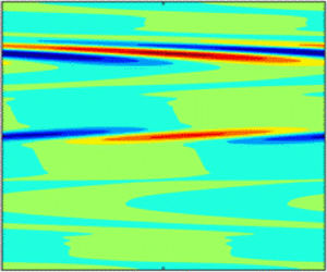
While the linear instability of classical diffusive convection (i.e. that in the absence of the phase boundary and shear) has been well understood, it is necessary to study this problem from the perspective of transient energy evolution before proceeding to the investigation on the effects of phase boundary and shear. As mentioned before, diffusive convection can bifurcate into steady convection for weak salinity stratification or into overstable motions for intense salinity stratification. These two typical cases are illustrated in figures 4 and 5, in which we show the eigenspectra in the modal analysis, the transient energy growths in the non-modal analysis and the perturbed salinity fields. Note that when we consider the hydrostatic base state, we set m = 0. In the steady instability regime, all the instability modes are located at the core mode which corresponds to a zero phase speed. The transient energy evolves exponentially with time after an initial rapid growth. The reasons for the initial rapid growth has been examined by Konopliv et al. (Reference Konopliv, Lesshafft and Meiburg2018) in the fingering regime, which is due to the interaction between double diffusion and velocity fluctuation field, rather than due to the Orr mechanism or lift-up mechanism. The situation in the oscillatory instability regime is dissimilar. As shown in figure 5(a), there exist two most unstable modes lying on the either side of the core mode. They acquire the identical growth rate but the opposite phase speed. This is because the overstable motions, a standing oscillation in the form of internal gravity waves, are characterized by the periodic transitions between the clockwise and counterclockwise circulation patterns (Veronis Reference Veronis1965; Radko Reference Radko2013). One of the most unstable modes shown in the eigenspectrum results in the clockwise rolls while its counterpart results in the counterclockwise rolls. The periodic transition of overstable motions is evidenced by the oscillation of the transient energy evolution shown in figure 5(b). In this regard, Schmid & Langre (Reference Schmid and de Langre2003) have also observed oscillating transient evolution in the analysis of a generic case of coupled-mode flutter, and Predtechensky et al. (Reference Predtechensky, McCormick, Swift, Noszticzius and Swinney1994) have experimentally observed the periodic behaviour of double-diffusive convection in a Hele-Shaw cell. It is expected that the perturbed salinity field shown in figure 5(c) is distorted unidirectionally at a given instant, which is dissimilar to that in the steady instability regime shown in figure 4(c). Other notable feature distinguishing overstable motions from steady convection are that the initial transient amplification seems to disappear here, which we will discuss in detail in § 4.2.2.

Figure 4. Diffusive convection in steady instability regime: (a) eigenspectrum; (b) transient energy growth; (c) perturbed salinity field. The parameters are Ra = 1.005Rc, RS = 0.005Rc, k = γc, m = 0, Re = 0 and  $\varLambda$ = 0. Hereafter, Rc = 1707.763, γc = 3.116 and λ = 2 ${\rm \pi}$/k. In panel (b), two additional cases with Ra = 1.0048Rc and 1.0052Rc are shown for comparison.

Figure 5. As with figure 4 but in the oscillatory instability regime. The parameters are Ra = 1.0209Rc, RS = Rc, k = γc, m = 0.
To give an insight into the intrinsic transition of overstable motions between the clockwise and counterclockwise patterns, we perform a transient energy analysis in a cycle, as shown in figure 6, and plot a sequence of accompanying perturbed salinity profiles, as shown in figure 7. The transient energy analysis is explained in Appendix A. As shown in figure 6, there are four energy components, which are VT (VS) for the energy exchange between the hydrodynamic velocity field and the temperature (salinity) field, VD for the viscous dissipation and Prod for the energy transfer between the perturbed hydrodynamic field and the base flow.

Figure 6. Transient energy growth and transient energy budget versus time. The parameters are as with figure 5. VT (VS) is the energy transfer between the velocity fluctuation field and temperature (salinity) field, Prod is the energy production by the basic shear and VD is the viscous dissipation.

Figure 7. Time evolution of the perturbed salinity fields in a cycle. The corresponding times stamps of the plots are specified in figure 6.
It is noted that in contrast to VS, VT is always positive, indicating that the temperature stratification always releases its potential energy into the hydrodynamic field, regardless of whether the fluid parcel is moving upwards or downwards. This is because the high diffusivity of heat allows the fluid parcel to quickly adjust its temperature to the environment. As with the transient energy G, the transient energy budgets also exhibit periodic oscillation, except that Prod is always zero as we consider a hydrostatic base state here. The dominant energy balance is between the heat diffusion and viscous dissipation. However, it is the energy exchange between the hydrodynamic field and salinity stratification (rather than temperature stratification) that acts in phase with G. This is because the overstable motions benefit from the low diffusivity of salt (Veronis Reference Veronis1965). A cycle of overstable oscillation clearly contains two oscillations of the transient energy G; one corresponds to the clockwise cell while the other to the counterclockwise cell. As shown in figure 6, the first oscillation of G (let us assume it is clockwise) starts with the increase of VS which is initially negative. When VS becomes positive, namely the salinity stratification starts to transform its potential energy into kinetic energy, the transition from clockwise to counterclockwise cells occurs, which is visualized in figure 7(c–g). After this transition, the newly generated counterclockwise cell increases in intensity until the peak (labelled as ‘h’ in figure 6) is reached. As the energy production by salt diffusion is reduced and finally the salinity field begins to absorb energy from the hydrodynamic field, the intensity of the counterclockwise rolls is weakened, thereby leading to another transition from counterclockwise to clockwise cell. The second transition is visualized in figure 7(k–o).
4.2 The effects of phase boundary
Regarding the effects of an ice–water interface on diffusive convection, we first have a look at the stability boundary shown in figure 8. Davis et al. (Reference Davis, Müller and Dietsche1984) pointed out that the effect of a steady solid–liquid interface on the buoyancy-driven instability in its underlying liquid layer is determined by the temperature difference between the liquid and solid layers, i.e.  $\varLambda$, which is equal to the solid thickness in the equilibrium state. Since the solid–liquid interface becomes a worse thermal conductor as $\varLambda$ increases, the critical Rayleigh number Rac and the critical wavenumber γc which mark the onset of flow motion are decreasing functions of $\varLambda$ (Davis et al. Reference Davis, Müller and Dietsche1984).

Figure 8. Effects of phase boundary on the convection threshold of diffusive convection: (a–c) low-RS cases; (d) and (e) high-RS cases. In panel (b), VT (VS) is the energy transfers between the velocity fluctuation field and temperature (salinity) field, Prod is the energy production by the basic shear and VD is the viscous dissipation. In panel (e), ΔRac denotes the difference between Rac for conducting boundary and phase boundary. Here, Re = 0 and m = 0.
In double-diffusive cases, the effect of a phase boundary on the convection threshold is more complex, which depends not only on  $\varLambda$, but also on RS. When RS is relatively low, as shown in figure 8(a and b), (Rac, γc) also decreases with larger values of $\varLambda$, which is qualitatively consistent with the results of Hirata et al. (Reference Hirata, Goyeau and Gobin2012) who studied the onset of double-diffusive convection in an under-ice melt pond. The decrease of Rac can be explained by a modal energy analysis shown in figure 8(c). The derivation of perturbation energy equation is given in Appendix A. The notation Prod, VD, VT and VS represent the same energy components as the transient energy analysis. We highlight the energy difference between $\varLambda$ > 0 and $\varLambda$ = 0, and to isolate the effects of $\varLambda$, all the parameters except $\varLambda$ are kept constant. It is readily seen that as $\varLambda$ increases, energy production by heat diffusion (VT) is increased. The increasing potential energy released from the unstable temperature stratification is more than that collected and stored by the stable salinity stratification. A part of this difference is dissipated by viscosity, while the remaining is transferred into the perturbation kinetic energy, driving the amplification of overstable oscillations.
In high-RS cases, however, we find that the presence of an ice–water interface tends to stabilize the system, despite that this effect is too small to make a real difference since Rac is very high in this situation. Therefore, it is deduced that in oceanic systems where RS is relatively high, the existence of an ice–water interface has negligible effects on the linear stability of the subglacial diffusive convection. In other contexts, where RS is relatively low (for example, the solidification of binary alloy), the existence of a phase boundary can change the heat flux at the interface so that the convection threshold will be decreased in a certain degree.
It is interesting to study the transition between steady and oscillatory instability regimes. In figure 9, we plot the magnified view of figure 8(a) in the low-RS regime. According to (3.20) (Veronis Reference Veronis1965), the transition from steady convective instability to oscillatory instability occurs at RS/Ra((β + Pr)/(1 + Pr)) = β, which is simplified to be Ra = 91RS for β = 0.01 and Pr = 10. In the case of a perfectly conducting boundary, our calculation follows this prediction well, as shown by figure 9(a). However, in the presence of a phase boundary, the transition is modified and the parameter range in which the conductive state is linearly unstable to steady convection is expanded, as shown in figure 9(b).

Figure 9. Magnified view of figure 8: (a) case with a conducting boundary; (b) case with a phase boundary.
The effects of phase boundary on transient energy growth in the oscillatory instability regime are illustrated in figure 10. It is seen that the ice–water interface does not change the oscillatory nature of overstable motions. However, an originally decaying oscillatory mode with a perfectly conducting boundary will become linearly unstable when considering an ice–water interface, which is consistent with the result of the modal analysis in low-RS cases where the phase boundary can decrease the threshold of diffusive convection. Furthermore, it is found that with the increase of ice thickness, the frequency of overstable oscillation will be decreased, as shown in figure 10(c).

Figure 10. (a,b) Effects of phase boundary on transient energy growth; (c) frequency of overstable oscillation f 1 as a function of  $\varLambda$. Here, k = γc and m = 0.
4.3 The effects of shear
Now we turn to examine the effects of Kolmogorov flow on the diffusive instability. To isolate the effects of the shear, we set  $\varLambda$ = 0. Before investigating the thermohaline-shear instability identified by Radko (Reference Radko2016) from the perspective of instability nature (oscillatory or steady) and initial transient growth, we first consider cases of RS < 106 for which three different instabilities are expected to occur for low (~0.1), moderate (~1) and high Re (~10).
4.3.1 Three instability regimes for RS < 106
When the shear intensity is weak, as shown in figure 11(a), the location of the most unstable modes in the eigenspectrum is analogous to the unsheared overstable motions and, compared with the remaining modes, they travel with the largest absolute phase speed. Moreover, as shown in the inserted perturbed salinity fields in figure 11(a), these two instability modes are triggered at y = 2/5 and 3/5, which is different from 1/4 and 3/4 predicted by Radko (Reference Radko2016). This might be because Radko (Reference Radko2016) considered the instability of transverse rolls with the vertical direction being periodic, while we consider here the instability of oblique rolls with the vertical boundary being no-slip. Nevertheless, it is believed that these two modes pertain to the oscillatory instability instead of the steady convective or Kelvin–Helmholtz instability, which is evidenced by the oscillatory behaviour of transient energy growth G and the accompanying energy budget E shown in figure 11(b and c). However, as shown in figure 11(b), the frequency of overstable oscillation is decreased for larger values of Re, which implies that the shear is prone to inhibiting the overstable oscillation here.

Figure 11. Oscillatory diffusive instability in the presence of Kolmogorov flow: (a) eigenspectra for a growing and a decaying case; (b) transient energy growths versus time; (c) transient energy budget versus time for Re = 0.04. The remaining parameters are Ra = 1.027Rc, RS = Rc,  $\varLambda$ = 0, k = γc × (1/3)0.5, m = γc × (2/3)0.5.
It should be clarified that the oscillatory behaviour identified here is dissimilar to that of Radko (Reference Radko2019). While Radko (Reference Radko2019) also found that the exponential growth of the quadratic perturbation norm is modulated on small time scales, this modulation in fact has an angular frequency twice that of the background shear which has a time-dependent amplitude. Therefore, we argue that the oscillation of Radko (Reference Radko2019) should be attributed to the time-dependent nature of the basic shear, whereas the oscillation shown in our study is inherited from the oscillatory nature of the overstable motions.
The diffusive instability in the presence of Kolmogorov flow of moderate intensity is displayed in figure 12. Unlike the low-Re cases, as shown in figure 12(a), there exists only one most unstable mode, located on the core-mode branch which has zero phase speed. This suggests that the instability is triggered at y = 1/2 where the basic velocity is zero but the shear rate is the largest. Since the Kelvin–Helmholtz instability by the Kolmogorov flow is negligible for Re = 1, the instability shown here is still buoyancy driven. Specifically, here the diffusive instability is steady rather than oscillatory, which is evidenced by the smooth growth of G shown in figure 12(b). The transient energy budget shown in figure 12(c) suggests that in the presence of moderate-Re Kolmogorov flow, the energy productions by the basic shear and salt diffusion are negligible in comparison to the energy balance between the heat diffusion and viscous dissipation. In this situation, the diffusive convection behaves like a single-component flow (e.g. Rayleigh–Bénard convection), despite that the circulation patterns in the present case are affected by the shear. The perturbed salinity field shown in figure 13 indicates that the system develops initially as the multi-cells pattern which will not persist for long. As time progresses, the system evolves to a stable circulation pattern, consisting of large-size cells localized at y = 1/2, and the perturbed energy starts to grows/decays exponentially with time.


Figure 13. Time evolution of salinity field for the case of Ra = 1.2Rc in figure 12.
Once the intensity of the basic shear is sufficiently strong, the fluid system might be susceptible to the dynamic instability induced by the basic shear itself, which refers to Kelvin–Helmholtz instability for Kolmogorov flow. Figure 14 illustrates this situation. Looking at figure 14(a), one finds that, while the original Kelvin–Helmholtz instability modes remain and are still the most unstable, the presence of double diffusion generates a large number of new modes. These new modes lead to the initial fast growth of G, as shown in figure 14(b). This transient amplification is due to the overstable motions generated at the initial instant, which is evidenced by the oscillation of transient energy budget Ek shown in figure 14(c). From figure 14(c), it is seen that the energy production by the basic shear is always positive, which is consistent with the idea that the high-Re Kolmogorov flow is a destabilizing forcing in the present system. In the long term, this forcing is dominant and the kinetic energy transferred from the basic shear into the perturbed hydrodynamic field is mainly compensated by the viscous dissipation. In the short term, however, the potential energy released/stored by the double-diffusive stratification is considerable and has the propensity to govern the initial dynamics. This is visualized in figure 15 where we display the time evolution of the perturbed salinity field. At t = 10, a pair of convective rolls arise in the upper region of the domain while the middle region is nearly uniform, implying that the oscillatory instability is triggered faster than the Kelvin–Helmholtz instability. As time progresses, this pair of rolls become distorted and elongated while simultaneously, near the inflection point of basic velocity profile (i.e. y = 1/2), the Kelvin–Helmholtz vortices set in. Subsequently, the overstable motions decrease in amplitude and gradually disappear, whereas the emerging Kelvin–Helmholtz streaks are intensified and eventually become dominant. Therefore, in the asymptotic stage, one observes in figure 14(b) a smooth growth of G similar to the case without double diffusion and in figure 15(d), the typical Kelvin–Helmholtz pattern.

Figure 14. Kelvin–Helmholtz instability subject to double diffusion: (a) eigenspectra in the presence/absence of double diffusion; (b) accompanying transient energy growths versus time; (c) transient energy budget for the case with double diffusion. The parameters are Re = 50.6, k = 3.262, m = 0. For the case with double diffusion, we have Ra = 1984, RS = 100Rc.

Figure 15. Time evolution of salinity field for the case with double diffusion in figure 14.
Preceding discussions characterize the properties of three instabilities that can arise in the present system, i.e. the oscillatory, steady and Kelvin–Helmholtz instabilities. To determine the boundaries distinguishing them, we present the stability maps for various shear intensity in figure 16. Regarding the transition from oscillatory to steady convective instability, it is found that there exist two paths of transition in the present system. (i) For the low-Re case, as shown in figure 16(a), the system first bifurcates into overstable motions, which, as with in the nonsheared case (Balmforth et al. Reference Balmforth, Ghadge, Kettapun and Mandre2006), will be superseded by the steady convection once Ra exceeds a critical value. (ii) Likewise, increasing the shear intensity, one will find a critical Re above which the steady convection is the only linear instability. This critical Re is located at the so-called codimension-two point (Predtechensky et al. Reference Predtechensky, McCormick, Swift, Noszticzius and Swinney1994), which connects the two paths of the transition from oscillatory to steady instability. The codimension-two points of the neutral curves for various RS constitute a curve which grows with increasing RS; see figure 16(b). One notable difference between the two paths is that the first path is valid for rolls with arbitrary orientation, whereas the second path is only valid for rolls with a transverse component since the shear has no effect on the longitudinal rolls; see the vertical curve in figure 16(b). In other words, in the presence of shear, longitudinal rolls are always oscillatory as long as (Ra, RS) are lying in the oscillatory instability regime determined by (3.20b), whereas the transverse and oblique rolls might be either oscillatory or steady, depending on both the buoyancy and the shear intensity.

Figure 16. (a) Boundaries of oscillatory and steady instabilities of transverse rolls for RS = 100Rc; (b) critical Re at codimension-two point for various RS, with TRs being the transverse rolls (m = 0), ORs the oblique rolls (we consider k = m) and LRs the longitudinal rolls (k = 0); (c) transition from diffusive instability to Kelvin–Helmholtz (KH) instability for RS = 100Rc. The vertical dashed line marks the transition of transverse rolls from the diffusive instability to the mixed (diffusive and Kelvin–Helmholtz) instability region.
The transition from buoyancy-driven instability to dynamic instability is illustrated in figure 16(c). Since the modal stability of longitudinal rolls are unaffected by the shear, longitudinal rolls are always unstable to the diffusive instability. For perturbations with a transverse component, the transition from diffusive instability to dynamic instability is observed. As shown in figure 16(c), there exist four distinct regions in the Ra–Re plane which correspond to the linearly stable region, diffusive instability region, Kelvin–Helmholtz instability region, and the mixed diffusive and Kelvin–Helmholtz instability region. In the diffusive instability region, buoyancy is the only destabilizing factor and likewise, high-Re Kolmogorov flow is the only destabilizing factor in the Kelvin–Helmholtz instability region. In the mixed region, both buoyancy and shear will contribute to the destabilization of the system. Since the Kelvin–Helmholtz instability is two-dimensional with m = 0, the transition to Kelvin–Helmholtz instability occurs at a higher Re for oblique rolls in comparison to the transverse rolls.
4.3.2 Transient growth for RS < 106
We are now able to explain a contradiction arising in § 4.3.1 which is concerned with the initial transient growth of G. As mentioned before, Konopliv et al. (Reference Konopliv, Lesshafft and Meiburg2018) evaluated the initial transient growth of the fingering convection and attributed it to a mechanism relying on the existence of density gradients. While we also detect this rapid growth in steady instability regime in the absence of shear and in the Kelvin–Helmholtz instability regime, it appears to be eliminated in low- and moderate-Re cases shown in figures 11 and 12.
Let us recall the transient growth mechanism of Konopliv et al. (Reference Konopliv, Lesshafft and Meiburg2018), i.e. ‘The fast initial growth occurs when θ* and s* initially have opposite signs, so they act in phase on the density field… As a result, v* grows strongly, which in turn will cause θ* and s* to move in the same direction until they eventually are of the same sign and sufficiently larger for the transient growth to decay.’ This description is highly consistent with our observation in figure 6 where we show the transient energy budget of overstable oscillation, despite that in Konopliv et al. (Reference Konopliv, Lesshafft and Meiburg2018), no stable oscillation in the long term but only an initial fast growth is observed. This indicates that the so-called transient growth mechanism of double-diffusive convection by Konopliv et al. (Reference Konopliv, Lesshafft and Meiburg2018) is in fact the mechanism responsible for the generation of the overstable motions. In other words, in a double-diffusive system, the optimal initial condition to achieve the maximum transient growth must be susceptible to the overstable motions, despite that unlike the diffusive configuration, this periodic flow might not persist too long in fingering convection. Therefore, it is expected that in the presence of shear, the optimal initial condition must be the longitudinal rolls since the shear tends to inhibit the oscillatory instability with a transverse component, as discussed in last section. This is evidenced by figure 17(a) where we show the contours of G as in the k-m plane in moderate-Re case. Now it is easy to deduce that the initial transient growth in figures 11 and 12 being insignificant is because we consider oblique rolls there. Furthermore, a conclusion can be drawn that regardless of the existence of a shear and of the instability type (oscillatory, steady or dynamic), the initial transient growth is exactly the first growth of G in a cycle of overstable oscillation, i.e. the growing stage in figure 6(a–h). In the oscillatory instability regime, particularly, this transient growth as well as the subsequent decay will repeat themselves over and over again, thereby leading to the so-called overstable motions. The effects of (Ra, RS, Re) on the transient growth is shown in figure 17(b). It is seen that the larger values of Ra or smaller values of RS result in a larger Gm (Gm = max(G) in a decaying or neutral case) since they correspond to a stronger buoyancy force. However, a more intense shear intensity also yields a larger Gm, which might be due to the lift-up mechanism, despite that this mechanism cannot induce the initial transient growth in pure Kolmogorov flow.

Figure 17. (a) Dependence of Gm on the horizontal wavenumber (k, m) with Gm = max(G), Ra = 2385, RS = 40Rc and Re = 1; (b) Gm as a function of m; (c and d) Gm/max(Gm) as a function of m where Gm = max(G) for a decaying case. In panel (d), Ra = 1.7Rc and RS = 80Rc.
It is noted that in many other sheared complex fluid systems, the longitudinal rolls also achieve the maximum transient growth, e.g. Jerome et al. (Reference Jerome, Chomaz and Huerre2012) for Rayleigh–Bénard–Poiseuille/Couette flow and Zhang et al. (Reference Zhang, Martinelli, Wu, Schmid and Quadrio2015) for electro-convection with Poiseuille flow. However, transient growth in these systems is subsequently different than our present system since they are due to the Orr mechanism or lift-up mechanism and relies on the existence of high-Re shear. In modal analysis, the longitudinal rolls are unaffected by the background shear, which is valid for the present system as with the aforementioned sheared convective flows. However, the non-modal results indicate that the buoyancy or Coulomb force has non-negligible effects on the initial transient growth by the Orr mechanism or lift-up mechanism. Specifically, in the lift-up mechanism, the optimal wavenumber to achieve the maximum transient growth is independent of shear intensity, but is influenced by the strength of the force that drives the convective motions (Jerome et al. Reference Jerome, Chomaz and Huerre2012; Zhang et al. Reference Zhang, Martinelli, Wu, Schmid and Quadrio2015). In the transient growth mechanism for a double-diffusive system (let us call it an overstable mechanism), more complex behaviours are expected. Regarding the effects of buoyancy on the optimal wavenumber, as shown in figure 17(c), it is seen that increasing Ra or equivalently decreasing RS results in a larger optimal wavenumber. As for the effect of shear, it is found that the low- (not shown here) and moderate-Re Kolmogorov flow has negligible effects on the optimal initial condition whereas in the case of the high-Re Kolmogorov flow, a larger optimal wavenumber is required to achieve to the maximum transient growth; see figure 17(d).
4.3.3 Thermohaline-shear instability
In this section, we consider a more realistic situation and investigate the effects of shear on diffusive instability in the context of oceanography where Ra and RS are much higher than those considered in §§ 4.3.1 and 4.3.2. The typical parameters of diffusive convection in high-latitude oceans are 1.5 < Rρ < 10 and 1 < Ri < 10, Pe ~ 103, where Rρ is the background density ratio, Ri the Richardson number and Pe the Péclet number (Radko Reference Radko2016). After a simple transformation from the term of Rρ–Ri–Pe formulation to the term of Ra–RS–Re formulation, we deduce that 105 < Ra < 106, 1.5 × 10⁷ < RS < 109, Re ~ 100. Here we considered RS ~ 108, while Re and Ra are independent and dependent variables, respectively. Our aim is to identify whether the thermohaline-shear instability found by Radko (Reference Radko2016) is oscillatory or steady and to discuss whether the transition between different instability regimes is realistically expected in the ocean.
In figure 18, we show the stability diagram for the sheared diffusive convection as a function of Re for RS = 108, τ = 0.01 and Pr = 10. In contrast to figure 16, here the critical Ra is a decreasing function of Re. This implies that at each point of the stability boundary within 0 < Re < 140.4, the system is individually stable with respect to diffusive instability and to Kelvin–Helmholtz instability, but unstable to the superposed instability. This superposed instability is precisely the thermohaline-shear instability identified by Radko (Reference Radko2016), which favours the transverse disturbances. The non-modal analysis suggests that the thermohaline-shear instability is oscillatory for Re lower than 81, above which the instability is steady. The transition from oscillatory instability to steady instability occurs at a codimension-two point, which has been specified in figure 18(a). After collecting all the codimension-two points in a wide range of RS, we obtain the critical Re and critical Ra marking the transition from oscillatory to steady instability, as shown in figure 18(b). It is seen that the critical Re and critical Ra are the increasing functions of RS. Moreover, further increasing Re, the critical Ra will become negative after Re exceeds 140.4, marking the transition to the Kelvin–Helmholtz instability regime.

Figure 18. Transition from oscillatory to steady instability in high-RS case: (a) critical Ra as a function of Re for RS = 108; (b) critical Re and critical Ra for codimension-two point as a function of RS; (c) asymptotic energy budget along the stability boundary in panel (a).
Here, we perform an asymptotic energy analysis for thermohaline-shear instability. Different from Radko (Reference Radko2016), in which only Pe is varied and the remaining parameters are all fixed, we proceed along the linear instability boundary, along which both Ra and Re are varied. It is seen from figure 18(c) that there exist two different regimes in which the energy budgets are entirely different, and the transition between these two regimes coincides with the codimension-two point that distinguishes the oscillatory and steady instabilities. In the oscillatory instability regime, the ultimate energy resource to amplify disturbances is the heat diffusion. The energy production by the shear is negligible or even negative, but the presence of the background shear promotes the release of energy from the temperature gradient into the perturbed hydrodynamic field. This is consistent with the hypothesis of Radko (Reference Radko2016) that rationalizes the catalytic effects of shear on the transfer of potential energy into kinetic energy. In the steady instability regime, however, the basic shear directly produces energy to the perturbed hydrodynamic field as with in many dynamic instabilities such as Kelvin–Helmholtz instability or Tollmien–Schlichting instability. In this sense, different from its oscillatory counterpart which involves complex interaction between shear and double diffusion (i.e. the catalytic effect), the steady thermohaline-shear instability resembles more a simple superposition of instabilities due to buoyancy and shear. Clearly, the condition for the steady thermohaline-shear instability to occur is more restrictive than the oscillatory one, since it requires a higher intensity and special velocity profile (containing inflection points) of the background shear. Therefore, we argue that the generation of thermohaline staircases in the Arctic Ocean is more likely due to the mechanism inducing the oscillatory instead of steady thermohaline-shear instability. This argument is consistent with the result of Radko (Reference Radko2019) that the thermohaline-shear instability can be triggered by the interaction between double diffusion and an unbounded, time-dependent Couette flow.
Since the codimension-two point occurring in figure 18 is within the parameter ranges of the real oceanic systems and the sheared transverse rolls in this situation are the least stable, the transition from oscillatory to steady instability discussed here is realistically possible. However, the transition into Kelvin–Helmholtz instability regime is realistically impossible, because it requires a sufficient shear intensity which is not satisfied in oceanic conditions.
It is necessary to investigate when the transient growth by double diffusion becomes significant in destabilizing the present system. To this end, we examine the effects of RS and Re on Gm, considering transverse rolls. Different from the cases in figure 17, it is obvious that the optimal initial condition for thermohaline-shear instability favours the transverse rolls. As shown in figure 19(a), with the increase of RS, Gm first undergoes nonmonotonic variation and eventually approaches a fixed value that is larger than the low-RS case but is still of order 10. This is due to the fact that the oscillatory convection is the low-amplitude motion, independent of the strength of the stabilizing force which refers to RS here. When considering the presence of a base flow, it is found that Gm is increased by two orders of amplitude and a sudden jump of Gm at the codimension-two point is observed. Specifically, in the oscillatory instability regime where Gm is an increasing function of Re, the transient energy returns to the low-amplitude oscillation after the initial fast growth, see the case of Re = 40 shown in figure 19(b). In the steady instability regime where Gm decreases with larger values of Re, however, the transient energy of a marginally stable case in the long term maintains a level identical to Gm. Therefore, it is deduced that the initial transient growth has important influence on the oscillatory thermohaline-shear instability. The reasons are twofold: (i) from the perspective of modal stability, transverse rolls are the least stable in thermohaline-shear instability and (ii) from the perspective of non-modal stability, the presence of shear makes the amplitude of initial transient growth an order higher of the oscillatory convection. In contrast, the transient growth by double-diffusion has negligible effect on the steady instability which, in the marginally stable case, is of the amplitude identical to the transient growth. In addition to the energy resource of instabilities, this is another principle difference between the steady thermohaline-shear instability and the oscillatory one.

Figure 19. Effects of RS and Re on the transient growth by double-diffusion. In panel (a), the results for Re = 0 are obtained by setting Re = 1 but considering a hydrostatic base flow. All the cases in panels (a) and (b) are marginally stable, with the corresponding neutral stability curves shown in figures 8(d) and 18(a).
5. Conclusion
In this paper, we have studied the effects of a solid–liquid interface and a Kolmogorov flow on the diffusive instability, using modal and non-modal stability analyses as well as energy analysis. In the absence of the phase boundary and shear, we showed that, with the overstable motions transitioning from the clockwise to counterclockwise circulation patterns, the transient energy undergoes periodic oscillation, driven by the salinity field which alternates between releasing and storing potential energy. For steady convective instability, however, a smooth evolution of transient energy is observed.
Regarding the effects of the phase boundary, the change of critical Rayleigh number Rac depends on the thickness of the solid phase and the salinity Rayleigh number RS. Specifically, for relatively small RS (RS < 106), Rac is decreased with larger values of solid thickness, due to the increasing energy transfer from the temperature gradient to the perturbed hydrodynamic field. In the context of ice melting in polar regions where RS is relatively large, the presence of an ice–water interface tends to stabilize the diffusive instability. However, in the absence of basic shear, since the buoyancy force required to drive the convective flow for large RS is very strong, this stabilizing effect is in fact trivial. However, while the existence of a phase boundary does not change the oscillatory nature of overstable motions, it makes the underlying fluid more susceptible to steady convection instead of the oscillatory convection.
In the presence of shear, three instabilities could be dominant for relatively small RS at different values of Reynolds number Re, which are the oscillatory instability for Re ~ 0.1, steady convective instability for Re ~ 1 and Kelvin–Helmholtz instability for Re > 50. The properties of these instabilities have been studied from the perspective of transient energy evolution. Specifically, in the Kelvin–Helmholtz instability regime, it is found that the dynamic instability develops more slowly than the oscillatory instability. Therefore, in the early phase, the overstable motions will arise in the low-shear region, and yields an initial rapid growth and the short-term periodic oscillation of the transient energy. As time progresses, the buoyancy-driven patterns will be elongated and gradually disappear, while at the same time, Kelvin–Helmholtz streaks will be generated in the inflection point of the basic velocity profile and eventually the dynamic instability becomes dominant.
For relatively large RS, we examined the thermohaline-shear instability identified by Radko (Reference Radko2016). By inspecting the temporal evolution of disturbances, we found that the thermohaline-shear instability could transition from the oscillatory instability regime to the steady one, and this transition is realistically possible in the context of oceanography. The energy analysis along the neutral stability curve of thermohaline-shear instability suggested that in the oscillatory instability regime, the heat diffusion and viscous dissipation are dominant in energy balance, with energy production by shear being negligible. This result confirmed that the hypothesis proposed by Radko (Reference Radko2016) to explain the catalytic role of shear is reasonable when the thermohaline-shear instability is oscillatory. In the steady instability regime, however, the mean shear makes direct and considerable contribution to the energy to intensify instabilities. Therefore, the steady thermohaline-shear instability is more like a direct superposition of instabilities by shear and buoyancy. We have also investigated the mechanism of the initial transient growth driven by double-diffusion (Konopliv et al. Reference Konopliv, Lesshafft and Meiburg2018). Results imply that the optimal initial condition to achieve the maximum transient growth must be susceptible to the overstable motions. For relatively small RS, since the shear inhibits all disturbances with a transverse component, the optimal initial condition favours the longitudinal rolls. For relatively large RS when the thermohaline-shear instability is induced, the optimal initial condition favours the longitudinal rolls, and the initial transient growth, driven by double diffusion and enhanced by the basic shear, might have significant impact on oscillatory thermohaline-shear instability.
In the future, it is necessary to numerically/experimentally investigate whether a thermohaline-shear system that is stable to the oscillatory instability predicted by modal analysis could be destabilized by the initial transient growth. We intend to investigate the subcritical bifurcation of double-diffusive convection subject to shear by weakly nonlinear instability properties and the transition from convective instability to absolute instability of the present system.
Acknowledgements
C.L. acknowledges helpful discussions with Zhenze Yao.
Funding
This work is supported by the National Natural Science Foundation of China (grant nos 52076055, 5190651), and partially supported by the fundamental Research Funds for the Central Universities (grant no. FRFCU5710094020). M.Z. acknowledges the financial support of a grant from the Ministry of Education, Singapore (WBS No. R-265-000-689-114).
Declaration of interests
The authors report no conflict of interest.
Appendix A. Asymptotic and transient energy analyses
In many cases, energy analysis is instructive to interpret the mechanisms hiding behind the observations by modal and non-modal analysis. Generally, depending on the focused time scale, the energy analysis can be classified into the asymptotic energy analysis and its transient counterpart, which will be briefly introduced here following Zhang et al. (Reference Zhang, Martinelli, Wu, Schmid and Quadrio2015). The asymptotic energy analysis focuses on the dynamics of perturbation energy in the limit of an infinite time horizon. The accompanying governing equation is obtained by multiplying the linearized momentum equation by its complex conjugate velocity  $v_i^{\dagger}$, i.e.
 \begin{align}v_i^{\dagger} \frac{{\partial {v_i}}}{{\partial t}} + v_i^{\dagger} {v_j}\frac{{\partial {{\bar{U}}_i}}}{{\partial {x_j}}} + v_i^{\dagger} {\bar{U}_j}\frac{{\partial {v_i}}}{{\partial {x_j}}} =- v_i^{\dagger} \frac{{\partial p}}{{\partial {x_i}}} + \frac{1}{{Re}}v_i^{\dagger} \frac{{{\partial ^2}{v_i}}}{{x_j^2}} + \frac{{Ra}}{{R{e^2}Pr}}v_i^{\dagger} \theta {x_i} - \frac{{{R_S}\beta }}{{R{e^2}Pr}}v_i^{\dagger} s{x_i}.\end{align}
Taking the complex conjugate of the above equation and then averaging the resulting two equations, we have
 \begin{align}
\dfrac{1}{2}\dfrac{\partial }{{\partial t}}v_i^{\dagger} {v_i} &
=- \dfrac{1}{2}(v_i^{\dagger} {v_j} + v_j^{\dagger}
{v_i})\dfrac{{\partial {{\bar{U}}_i}}}{{\partial {x_j}}} -
\dfrac{1}{{Re}}\dfrac{{\partial v_i^{\dagger} }}{{\partial
{x_j}}}\dfrac{{\partial {v_i}}}{{\partial {x_j}}}\notag\\ &\quad +
\dfrac{1}{2}\dfrac{{Ra}}{{R{e^2}Pr}}(\theta v_i^{\dagger} +
{\theta ^{\dagger} }{v_i}){x_i} - \dfrac{1}{2}\dfrac{{{R_S}\beta
}}{{R{e^2}Pr}}(v_i^{\dagger} s + vs_i^{\dagger} ){x_i}\notag\\ & \quad +
\dfrac{\partial }{{\partial {x_j}}}\left[ { -
\dfrac{1}{2}v_i^{\dagger} {v_i}{{\bar{U}}_j} -
\dfrac{1}{2}(\,pv_i^{\dagger} + p_i^{\dagger} {v_i}){\delta_{ij}} +
\dfrac{1}{{\textrm{2}Re}}\left( {v_i^{\dagger} \dfrac{{\partial
{v_i}}}{{\partial {x_j}}} + {v_i}\dfrac{{\partial v_i^{\dagger}
}}{{\partial {x_j}}}} \right)} \right],
\end{align}
\begin{align}
\dfrac{1}{2}\dfrac{\partial }{{\partial t}}v_i^{\dagger} {v_i} &
=- \dfrac{1}{2}(v_i^{\dagger} {v_j} + v_j^{\dagger}
{v_i})\dfrac{{\partial {{\bar{U}}_i}}}{{\partial {x_j}}} -
\dfrac{1}{{Re}}\dfrac{{\partial v_i^{\dagger} }}{{\partial
{x_j}}}\dfrac{{\partial {v_i}}}{{\partial {x_j}}}\notag\\ &\quad +
\dfrac{1}{2}\dfrac{{Ra}}{{R{e^2}Pr}}(\theta v_i^{\dagger} +
{\theta ^{\dagger} }{v_i}){x_i} - \dfrac{1}{2}\dfrac{{{R_S}\beta
}}{{R{e^2}Pr}}(v_i^{\dagger} s + vs_i^{\dagger} ){x_i}\notag\\ & \quad +
\dfrac{\partial }{{\partial {x_j}}}\left[ { -
\dfrac{1}{2}v_i^{\dagger} {v_i}{{\bar{U}}_j} -
\dfrac{1}{2}(\,pv_i^{\dagger} + p_i^{\dagger} {v_i}){\delta_{ij}} +
\dfrac{1}{{\textrm{2}Re}}\left( {v_i^{\dagger} \dfrac{{\partial
{v_i}}}{{\partial {x_j}}} + {v_i}\dfrac{{\partial v_i^{\dagger}
}}{{\partial {x_j}}}} \right)} \right],
\end{align}
where  $v_i^{\dagger} {v_i}/2$ is the perturbation energy density. The terms in the second line exert no influence on the energy balance for periodic, no-slip and no-penetration conditions (Zhang et al. Reference Zhang, Martinelli, Wu, Schmid and Quadrio2015). Therefore, after an integration over a control volume $\varOmega$, (A2) becomes
 \begin{align}
\dfrac{1}{2}\int_\varOmega {\dfrac{\partial }{{\partial
t}}v_i^{\dagger} {v_i}\,\textrm{d}V} & =-
\dfrac{1}{2}\int_\varOmega {(v_i^{\dagger} {v_j} + v_j^{\dagger}
{v_i})\dfrac{{\partial {{\bar{U}}_i}}}{{\partial
{x_j}}}\,\textrm{d}V} \ldots \ldots \ldots \ldots \ldots
\textrm{Prod}\notag\\ & \quad - \dfrac{1}{{Re}}\int_\varOmega
{\dfrac{{\partial v_i^{\dagger} }}{{\partial
{x_j}}}\dfrac{{\partial {v_i}}}{{\partial
{x_j}}}\,\textrm{d}V} \ldots \ldots \ldots \ldots \ldots
\ldots \ldots \ldots \ldots \ldots\textrm{VD}\notag\\ & \quad
+ \dfrac{1}{2}\dfrac{{Ra}}{{R{e^2} \cdot Pr}}\int_\varOmega
{(\theta v_i^{\dagger} + {\theta ^{\dagger}
}{v_i}){x_i}\,\textrm{d}V} \ldots \ldots \ldots \ldots
.\textrm{VT}\notag\\ & \quad - \dfrac{1}{2}\dfrac{{Ra \cdot \beta
}}{{R{e^2} \cdot Pr}}\int_\varOmega {(sv_i^{\dagger} + {s^{\dagger}
}{v_i}){x_i}\,\textrm{d}V} \ldots \ldots \ldots \ldots
.\textrm{VS},
\end{align}
\begin{align}
\dfrac{1}{2}\int_\varOmega {\dfrac{\partial }{{\partial
t}}v_i^{\dagger} {v_i}\,\textrm{d}V} & =-
\dfrac{1}{2}\int_\varOmega {(v_i^{\dagger} {v_j} + v_j^{\dagger}
{v_i})\dfrac{{\partial {{\bar{U}}_i}}}{{\partial
{x_j}}}\,\textrm{d}V} \ldots \ldots \ldots \ldots \ldots
\textrm{Prod}\notag\\ & \quad - \dfrac{1}{{Re}}\int_\varOmega
{\dfrac{{\partial v_i^{\dagger} }}{{\partial
{x_j}}}\dfrac{{\partial {v_i}}}{{\partial
{x_j}}}\,\textrm{d}V} \ldots \ldots \ldots \ldots \ldots
\ldots \ldots \ldots \ldots \ldots\textrm{VD}\notag\\ & \quad
+ \dfrac{1}{2}\dfrac{{Ra}}{{R{e^2} \cdot Pr}}\int_\varOmega
{(\theta v_i^{\dagger} + {\theta ^{\dagger}
}{v_i}){x_i}\,\textrm{d}V} \ldots \ldots \ldots \ldots
.\textrm{VT}\notag\\ & \quad - \dfrac{1}{2}\dfrac{{Ra \cdot \beta
}}{{R{e^2} \cdot Pr}}\int_\varOmega {(sv_i^{\dagger} + {s^{\dagger}
}{v_i}){x_i}\,\textrm{d}V} \ldots \ldots \ldots \ldots
.\textrm{VS},
\end{align}where Prod represents the energy transfer between the perturbed hydrodynamic field and the basic shear, VD the energy dissipated by viscosity, and VT (VS) the potential energy released from temperature (salinity) stratification into the velocity fluctuation field.
Different from the asymptotic one, transient energy analysis focuses the dynamics of the perturbed kinetic energy inside a finite time horizon. The evolution of the accompanying energy density is defined as (e.g. Zhang et al. Reference Zhang, Martinelli, Wu, Schmid and Quadrio2015)
 \begin{align}
\dfrac{1}{{|\varOmega |}}\int_\varOmega {\dfrac{{\partial
{E_k}}}{{\partial t}}\,\textrm{d}V} &= \dfrac{1}{{|\varOmega
|}}\int_0^1 {\int_0^{2{\rm \pi} /k} {\int_0^{2{\rm \pi} /m}
{\dfrac{\partial }{{\partial t}}} } \left( {\dfrac{{{u^2} +
{v^2} + {w^2}}}{2}} \right)\textrm{d}V} \notag\\ &\quad =
\dfrac{1}{{|\varOmega |}}\int_0^1 \int_0^{2{\rm \pi} /k}
\int_0^{2{\rm \pi} /m} \left[ -
uv\dfrac{{\textrm{d}U}}{{\textrm{d}y}} -
\dfrac{1}{{Re}}\dfrac{{\partial {u_i}}}{{\partial
{x_j}}}\dfrac{{\partial {u_i}}}{{\partial {x_j}}}\right. \notag\\ &\quad + \left.
\dfrac{{Ra}}{{R{e^2}Pr}}v\theta - \dfrac{{{R_S}\beta
}}{{R{e^2}Pr}}vs
\right]\textrm{d}z\,\textrm{d}\kern0.7pt x\,\textrm{d}y ,
\end{align}
\begin{align}
\dfrac{1}{{|\varOmega |}}\int_\varOmega {\dfrac{{\partial
{E_k}}}{{\partial t}}\,\textrm{d}V} &= \dfrac{1}{{|\varOmega
|}}\int_0^1 {\int_0^{2{\rm \pi} /k} {\int_0^{2{\rm \pi} /m}
{\dfrac{\partial }{{\partial t}}} } \left( {\dfrac{{{u^2} +
{v^2} + {w^2}}}{2}} \right)\textrm{d}V} \notag\\ &\quad =
\dfrac{1}{{|\varOmega |}}\int_0^1 \int_0^{2{\rm \pi} /k}
\int_0^{2{\rm \pi} /m} \left[ -
uv\dfrac{{\textrm{d}U}}{{\textrm{d}y}} -
\dfrac{1}{{Re}}\dfrac{{\partial {u_i}}}{{\partial
{x_j}}}\dfrac{{\partial {u_i}}}{{\partial {x_j}}}\right. \notag\\ &\quad + \left.
\dfrac{{Ra}}{{R{e^2}Pr}}v\theta - \dfrac{{{R_S}\beta
}}{{R{e^2}Pr}}vs
\right]\textrm{d}z\,\textrm{d}\kern0.7pt x\,\textrm{d}y ,
\end{align}where Ek is the energy density. As before, the four terms in the square brackets in (A4) are denoted by Prod, VD, VT and VS, respectively, and they represent the same thing as in (A3).


