


1. Introduction
This study reports on the dynamics of a rigid flat plate that is (i) oriented parallel to a uniform and steady free stream, and (ii) mounted on a torsional spring at its trailing edge. This mechanical structure has a single degree of freedom: rotation of the plate about its trailing edge. It is termed a ‘rigid inverted flag’. A schematic of this simple system is provided in figure 1. The dynamics of this fluid–structure system is compared with that of the usual ‘inverted flag’, which consists of a flexible elastic sheet clamped at its trailing edge. This comparison enables the role of continuous sheet elasticity (many degrees of freedom) to be assessed and further exploration of the underlying physics of inverted flags. Many studies have examined the connection between the observed dynamic response of the (flexible) inverted flag and its vortex shedding. This has been performed numerically (for example, see Gurugubelli & Jaiman Reference Gurugubelli and Jaiman2015, Reference Gurugubelli and Jaiman2019) and experimentally (among others see Kim et al. Reference Kim, Cossé, Cerdeira and Gharib2013; Kang, Kim & Kim Reference Kang, Kim and Kim2017; Yu, Liu & Chen Reference Yu, Liu and Chen2017; Hu et al. Reference Hu, Wang, Wang and Breitsamter2019). Further, two studies have produced phase maps of the different dynamic responses. The numerical study of Shoele & Mittal (Reference Shoele and Mittal2016) showed a variety of vortex wake configurations, classified into four basic groups: SS, LS, SA and LA. The first letter designates the vibration amplitude: small (S) or large (L), while the second letter denotes symmetric (S) or asymmetric (A) responses about the undeformed flag position. Shoele & Mittal (Reference Shoele and Mittal2016) identified two LS states: (i) a high-mass state consisting of an apparently meandering vortex wake, and (ii) a low-mass state with a vortex dipole from the leading edge and a single vortex from the trailing edge shed at each half-cycle. A second numerical study of Goza, Colonius & Sader (Reference Goza, Colonius and Sader2018) used direct numerical simulations that incorporated stability analysis. This identified all of the equilibria (both stable and unstable) of the inverted flag system, and six primary response regimes as a function of flow speed and flag mass. Similar to Shoele & Mittal (Reference Shoele and Mittal2016), Goza et al. (Reference Goza, Colonius and Sader2018) reported two large-amplitude flapping states, one that was synchronised to the vortex shedding and another that was not – this difference correlated with the flag mass. Goza et al. (Reference Goza, Colonius and Sader2018) also showed that, for light flags, large-amplitude flapping was predominantly aperiodic/chaotic. It was reported that this chaos resulted from an apparently random switching between large-amplitude flapping and a state where the flag was statically deflected to one side, i.e. the deflected state.

Figure 1. Schematic of the rigid inverted flag, showing the flag dimensions,  $L$ and $h$; Cartesian coordinate system, $(x, y)$, and its origin at the plate's trailing edge; impinging flow in the $x$-direction; angle of rotation, $\theta$, about the torsional spring of stiffness per unit plate width, $k_\theta$, at the plate's trailing edge; and the semicircular ends used in the numerical method. The $z$-direction is out of the page.
We show that the rigid inverted flag produces similar dynamics and phase maps to the flexible inverted flag (Goza et al. Reference Goza, Colonius and Sader2018) with synchronised, subharmonic and chaotic responses. While the range of flow speeds over which these various states appear is different between rigid and flexible inverted flags, as may be expected, we find that a large proportion of the large-amplitude flapping responses of the rigid inverted flag are chaotic. The single degree-of-freedom mechanical system of the rigid inverted flag allows the interaction between a number of organising states to be identified, and we show that chaos in the rigid inverted flag can arise through several different mechanisms depending on the system parameters.
Sader et al. (Reference Sader, Cossé, Kim, Fan and Gharib2016a) presented evidence that the observed large-amplitude flapping of the flexible inverted flag is a vortex-induced vibration (VIV). Synchronisation between vortex formation and subsequent shedding from the leading (and trailing) edges, and the flag motion, is the primary phenomenon controlling this fluid–structure interaction. These mechanisms have been further investigated in the context of finite span flags (Sader, Huertas-Cerdeira & Gharib Reference Sader, Huertas-Cerdeira and Gharib2016b) and those with different planform shapes (Fan et al. Reference Fan, Huertas-Cerdeira, Cossé, Sader and Gharib2019). However, the position of VIV as a governing phenomenon has been challenged in recent work from Tavallaeinejad et al. (Reference Tavallaeinejad, Païdoussis, Legrand and Kheiri2020a,Reference Tavallaeinejad, Païdoussis, Salinas, Legrand, Kheiri and Botezb). These authors argue that, at least for heavy flags, the mechanism is not VIV but is instead related to coupled-mode flutter-like instabilities, or a movement-induced excitation (Naudascher & Rockwell Reference Naudascher and Rockwell1994; Païdoussis Reference Païdoussis2014, Reference Païdoussis2016).
We show that similar response regimes occur for rigid and flexible inverted flags. This finding suggests that similar fluid–structure mechanisms occur in both set-ups. The conventional flag – which is clamped at its leading edge – loses its stability through a coupled-mode flutter instability. The same mechanism obviously cannot occur for a rigid plate that is also clamped at its leading edge. The fact that the rigid inverted flag, with its single mechanical degree-of-freedom, exhibits large-amplitude flapping similar to that of a flexible inverted flag suggests that the usual framework for understanding the conventional flag may not necessarily apply.
Another potential framework for modelling the rigid inverted flag is to analyse it in terms of torsional galloping (Paidoussis, de Langre & Price Reference Païdoussis, de Langre and Price2011), i.e. with rotation occurring about its clamped trailing edge. While there has been some success in analysing the initial loss of stability of similar systems (see Fernandes & Armandei (Reference Fernandes and Armandei2014), and Tadrist et al. (Reference Tadrist, Julio, Saudreau and de Langre2015) in the context of the fluttering of leaves), it has not been possible to predict the dynamics of any large-scale flapping or torsional oscillation via a simplified model, and the full problem must be solved to capture the nonlinear dynamics. For example, a numerical study on torsional galloping of rectangular prisms is presented by Robertson et al. (Reference Robertson, Li, Sherwin and Bearman2003). Related work on autorotation and rotational flutter of plates, that are free to rotate about an axis at various distances from the leading edge, is given in Mirzaeisefat & Fernandes (Reference Mirzaeisefat and Fernandes2013), Jin et al. (Reference Jin, Ji, Liu and Chamorro2016) and Kumar, Poddar & Kumar (Reference Kumar, Poddar and Kumar2018).
Many studies have investigated the energy harvesting potential of flexible inverted flags assuming their bending energy can be harnessed by, for example, piezoelectric materials. For inverted flags, these studies include those by Shoele & Mittal (Reference Shoele and Mittal2016), Orrego et al. (Reference Orrego, Shoele, Ruas, Doran, Caggiano, Mittal and Kang2017), Gunasekaran & Ross (Reference Gunasekaran and Ross2019) and Silva-Leon et al. (Reference Silva-Leon, Cioncolini, Nabawy, Revell and Kennaugh2019), which follow the earlier work on conventional flags (Allen & Smits Reference Allen and Smits2001; Michelin & Doaré Reference Michelin and Doaré2013). Many of the results for both configurations are reviewed by Yu, Liu & Amandolese (Reference Yu, Liu and Amandolese2019). The fact that similar large-amplitude motions are observed here for the rigid inverted flag suggests that it too is a viable energy harvester. However, the rigid inverted flag has the potential to facilitate implementation and be more efficient in its energy conversion because of its single access point for mechanical deformation: its trailing-edge torsional spring. For example, rotation about this single axis can be used to drive a conventional electric generator. We also note that a rotating device will not suffer from fatigue failure that is inevitable in a bending-based device (Yang et al. Reference Yang, Cioncolini, Nabawy and Revell2021). Interestingly, this single-axis set-up does not appear to have been investigated experimentally.
The primary focus of this paper is to investigate the stability and dynamics of the rigid inverted flag using two-dimensional direct numerical simulations at a Reynolds number  ${\textit {Re}} = 200$. The study progresses as follows: section 2 outlines the problem set-up; a more complete description of the numerical method, domain and resolution tests are relegated to Appendix A. Section 3 then provides results from a series of simulations at different plate masses and flow speeds. This maps out the overall picture of the varying states and flow regimes that occur. A direct comparison and discussion of the rigid and flexible inverted flags is provided in § 3.3. Section 4 then gives detailed descriptions of the various states and regimes identified in § 3. Sections 4.1, 4.2 and 4.2.6 describe the steady and periodic organising states. A simple framework is presented in § 4.2.1 to explain the switch from a synchronised to a subharmonic state with increasing flag mass. This is developed in terms of the interaction of a natural frequency accounting for fluid inertia and a preferred vortex shedding frequency; with details of the consideration of linear fluid inertia presented in Appendix B. Sections 4.3 and 4.4 describe how these various organising states can interact and lead to chaotic oscillations, with § 5 providing some concluding remarks.
2. Problem definition and numerical method
A rigid inverted flag consists of a rigid two-dimensional flat, thin plate of length,  $L$, that rotates an angle, $\theta$, about a torsional spring of stiffness (per unit plate width), $k_\theta$, through an axis along its trailing edge. The entire set-up is immersed in an unbounded free stream of speed, $U$; see figure 1. The rest (undeflected) position of the flat plate is parallel to the incident flow, i.e. $\theta =0$. The flat plate has constant mass density, $\rho _s$, and small but finite (constant) thickness, chosen for convenience to be $h = 0.022 L$. Finite thickness is required for proper representation of the plate using the immersed-boundary method, summarised below and detailed in Appendix A; the plate ends have a semicircular profile, for the same reason.
Two-dimensional direct numerical simulations are performed of the incompressible Navier–Stokes equations, in the sharp-interface immersed-boundary method form
 \begin{equation} \boldsymbol{\nabla}\boldsymbol{\cdot}{\boldsymbol{u}} = 0,\quad \frac{\partial{\boldsymbol{u}}}{\partial t} ={-}{\boldsymbol{u}}\boldsymbol{\cdot}\boldsymbol{\nabla} {\boldsymbol{u}} - \frac{1}{\rho}\boldsymbol{\nabla} p + \nu\nabla^2{\boldsymbol{u}} + \frac{1}{\rho}\boldsymbol{F}_b, \end{equation}
where  $ {\boldsymbol {u}}$ is the velocity field, $p$ is the pressure field, $t$ is time, $\nu$ is the fluid kinematic viscosity and $\rho$ is the fluid density; $\boldsymbol {F}_b$ is a body force in the fluid domain, ensuring the flow matches the required boundary condition at the immersed solid boundary.
Structural motion of the rigid flag satisfies
 \begin{equation} \frac{{\rm d}^2\theta}{{\rm d} t^2} + \frac{k_\theta}{I}\theta = \frac{M}{I}, \end{equation}
where  $I$ is the mass moment of inertia per unit width of the flag about its trailing edge (axis), and $M$ is the moment per unit width about the same axis due to fluid forces; the latter term couples (2.1a,b) and (2.2).
This fluid–structure problem is uniquely specified by three dimensionless parameters. We follow the set of parameters used by Sader et al. (Reference Sader, Cossé, Kim, Fan and Gharib2016a). The Reynolds number is
 \begin{equation} {\textit{Re}} = \frac{UL}{\nu}, \end{equation}
while the respective mass ratio and dimensionless flow speed are
 \begin{equation} \mu = \frac{\rho L}{\rho_s h},\quad \kappa = \frac{\rho U^2 L^2}{k_\theta}. \end{equation}
The usual (dimensional) convective time scale of  $\tau = L/U$ is chosen; frequencies are normalised by this time scale.
In all simulations, the Reynolds number is fixed at  ${\textit {Re}} = 200$, similar to previous numerical studies of the flexible inverted flag (Ryu et al. Reference Ryu, Park, Kim and Sung2015; Shoele & Mittal Reference Shoele and Mittal2016). Three mass ratios are studied: (i) $\mu = 0.39$, identical to the inverted flag wind tunnel experiments of Sader et al. (Reference Sader, Cossé, Kim, Fan and Gharib2016a); (ii) $\mu = 2.27$; and (iii) $\mu = 4.54$, corresponding to systematically lighter flags. The dimensionless flow speed, $ {\kappa }$, is varied as the independent parameter. This corresponds to varying the torsional stiffness, $k_\theta$, at constant flow speed, similar to previous numerical studies outlined above.
3. Identification of dynamic regimes and their transitions
We begin our exploration of the rigid inverted flag's dynamics by reporting time domain simulations in figure 2 as a function of the dimensionless flow speed,  $\kappa$. A number of dynamic states are observed, but overall these simulations closely resemble the widely reported dynamics and transitions for flexible inverted flags. This observation suggests that plate flexibility, with its many degrees of freedom, is not an essential ingredient.

Figure 2. Time lapse images of the rigid inverted flag position showing a range of different dynamic states. The dimensionless flow speed,  $ {\kappa }$, increases from left to right, top to bottom. The exact parameters used for these images are the same as the examples marked on the regime maps of figure 4. Descriptions of each of these states are provided in §§ 4.1, 4.2 and 4.3. In all images, the flag rotates about its right edge and the flow direction is from left to right.
To summarise this dynamics, bifurcation diagrams of the rigid inverted flag dynamics are provided in figure 3. These are developed by recording the maxima/minima of the angular position,  $\theta$, over time. The diagrams have been shaded to highlight the different dynamic states: steady, small-amplitude periodic and chaotic and large-amplitude periodic and chaotic. Values of $ {\kappa }$ that are used for example cases in later sections are marked with vertical lines.

Figure 3. Bifurcation diagrams,  $\theta$ vs $\kappa$, (upper figures) constructed by extracting the values of maxima ( $\bullet$, blue) and minima ( $\bullet$, orange) in $\theta$, and spectrograms (lower figures) of the flag response as a function of the dimensionless flow speed, $ {\kappa }$, for (a) $\mu = 4.54$, (b) $\mu = 2.27$, (c) $\mu = 0.39$ (matching that of the experiments of Sader et al. (Reference Sader, Cossé, Kim, Fan and Gharib2016a) for the flexible inverted flag). Bifurcation diagrams: vertical dashed lines mark the divergence instability from inviscid theory, see (4.5). Grey and green shaded areas demarcate parameter ranges for shear-layer dominated states and large-amplitude flapping states, respectively. Red vertical lines mark the parameters used for example cases. See figure 4 for further explanation of these parameter ranges and example cases. Spectrograms: horizontal dashed lines mark the nominal vortex shedding frequency, $f_{vs} = 0.12$, and its first subharmonic, $f_{vs}/2 = 0.06$. Blue curves are a corrected natural frequency, $f_{N_{f}}$, that approximately accounts for fluid inertia, as defined in (4.9).
Corresponding spectrograms in figure 3 are generated by first calculating the frequency spectrum of the time series of the angular position,  $\theta$, for each simulation at a fixed $ {\kappa }$. Second, each spectrum is normalised by the magnitude of the largest frequency component. Finally, these normalised spectra (for each $\kappa$) are combined to produce the spectrograms (for all $\kappa$) in figure 3. This approach highlights variations in the dominant frequency component as a function of $ {\kappa }$. These spectrograms are annotated with (i) dashed lines marking a nominal vortex shedding frequency and its first subharmonic, and (ii) a solid line denoting a natural resonant frequency that incorporates a correction due of the surrounding fluid; as outlined in (4.9).
Figure 4 presents the shaded regions only of the bifurcation diagrams in figure 3, now with annotations labelling the states observed. Below each of these diagrams is a plot with vertical lines marking the values of  $ {\kappa }$ used in examples in later sections, and the state observed in each of these examples.

Figure 4. As for figure 3, showing the shaded regions of the bifurcation diagrams and annotations of the observed states. Example cases used in later sections are indicated by vertical lines in plots below each bifurcation diagram. Legend: steady regimes (white); periodic/chaotic small-amplitude oscillations driven by shear layer interactions (dark/light grey); periodic/chaotic large-amplitude oscillations with significant vortex shedding (dark/light green). Steady and periodic ranges are annotated with the state observed in that range. Chaotic ranges are labelled simply as chaotic – the interactions leading to chaos are a function of  $ {\kappa }$, hard boundaries are not provided for each of these interactions; (a) $\mu = 4.54$, (b) $\mu = 2.27$, (c) $\mu = 0.39$.
The results in figures 3 and 4 show that there are general features common for all mass ratios,  $\mu$, studied. For low flow speeds, $\kappa \lesssim 0.7$, the flag dynamics is governed by interaction of the shear layers on each side of the plate. The precise value of $ {\kappa }$ at which the dynamics ceases to be driven by these shear-layer interactions is weakly proportional to $\mu$. These regimes are represented by the left-most white and grey areas in figures 3 and 4. There is no distinct vortex shedding. As $\kappa$ increases, at least four states can be identified: state I is an undeformed or undeflected equilibrium, while state II is a deflected equilibrium. State III corresponds to small-amplitude flapping, which is biased to one side. Note that similar states (using the same terminology) are found for the flexible inverted flag in Goza et al. (Reference Goza, Colonius and Sader2018). However, for the rigid inverted flag, we find a fourth state which appears to be a heteroclinic orbit between the two manifestations of state III (one biased to the left and the other biased to the right). Further details of these shear-layer dominated states are presented in § 4.1.
For higher flow speeds,  $\kappa \gtrsim 0.7$, a wide variety of large-amplitude flapping states occur. The first distinction is between periodic and chaotic flapping. Ranges of $ {\kappa }$ where periodic oscillation occurs are marked with dark shading in figures 3 and 4, and $\kappa$-ranges where chaotic oscillations arise are lightly shaded. The chaotic regimes are not broken down into separate ranges for each type of chaotic interaction observed – hard boundaries in the parameter space where each occurs are not delineated. However, example cases of each type of interaction are provided, and the parameters of these example cases are marked in the second subplots of figure 4. This shows that the type of chaotic oscillation observed varies with $\kappa$.
Figures 3 and 4 also show that the set of large-amplitude states depends on the mass parameter,  $\mu$. We delineate between states for ‘higher’ and ‘lower’ $\mu$; corresponding to lighter and heavier flags, respectively. Both $\mu = 4.54$ and $\mu = 2.27$ correspond to higher- $\mu$ cases, with a similar progression of states with increasing $\kappa$. The progression for the lower value of $\mu = 0.39$ is distinctly different; this distinction is discussed further in §§ 3.1 and 3.2 below.
3.1. Lighter flags – higher mass ratios,  $\mu$
$\mu$

As  $\kappa$ increases, the first large-amplitude flapping state observed in both higher- $\mu$ cases is a periodic synchronised state (denoted $ {P_{1}}$ in figure 4a), where flapping is synchronised to the vortex shedding. This is marked in figures 3 and 4 by the dark green stripe over a range of $ {\kappa }$ starting just before $ {\kappa } = 0.8$. The extent of this range is observed to be inversely proportional to $\mu$. The synchronisation is suggestive of a VIV, as proposed by Sader et al. (Reference Sader, Cossé, Kim, Fan and Gharib2016a) for the flexible inverted flag and described as ‘mode IV’ in Goza et al. (Reference Goza, Colonius and Sader2018). This synchronised state is not observed for the lower- $\mu$ case of $\mu = 0.39$; a simple argument supporting this loss of synchronisation at low $\mu$ is presented in § 4.2.1. Details of this state are presented in § 4.2.3.
Figure 3 shows that as  $ {\kappa }$ is increased, this synchronised periodic state is followed by a regime of chaotic response (light green stripe in figures 3 and 4). This chaotic response is characterised by oscillation amplitudes that fluctuate around the value obtained for the synchronised $ {P_{1}}$ state. We propose that this chaotic response is driven by instability of the $ {P_{1}}$ limit cycle, producing type I intermittency (Pomeau & Manneville Reference Pomeau and Manneville1980) (as labelled in figure 4b). Details of this process are presented in § 4.3.1.
Following this chaotic response is a very narrow band near  $ {\kappa } = 1$ where a periodic state is again recovered. This state is distinct from $ {P_{1}}$, because it is asymmetric. The bifurcation diagrams of figure 3 show that it has two local maxima and one minimum per oscillation cycle; it is denoted the $ {P_{2_{A}}}$ state (as labelled in figure 4a). Details of this state are presented in § 4.2.4.
The next feature as  $ {\kappa }$ increases further is a large band of $ {\kappa }$ where chaotic oscillations reappear, before the onset of the periodic laid-over (deflected) state $ {D}$. Figures 3 and 4 show that a chaotic dynamics dominates the range of $ {\kappa }$ studied. However, the nature of the chaos is not uniform across this entire range. Chaos via mode competition occurs depending on the value of $ {\kappa }$. For $\kappa$-values at the low end of this range (just above $ {\kappa } = 1$) there is competition between the two manifestations of $ {P_{2_{A}}}$: one with a positive mean and one with a negative mean. For $ {\kappa } \approx 1.8$, there is competition between the manifestations of $ {P_{2_{A}}}$ and a spatio-temporally symmetric, but subharmonic state $ {P_{2}}$. This is despite the subharmonic state $ {P_{2}}$ never being observed as a stable state for high $\mu$; it is, however, observed for low $\mu$ as described in § 3.2. For higher $ {\kappa } \approx 2.2$, there is competition between the subharmonic $ {P_{2}}$ and the deflected state $ {D}$. For $ {\kappa } \approx 2.3$ and above there is competition between the two manifestations of $ {D}$; again, one with a negative and one with a positive mean. These interactions are labelled at sample locations on figure 4, and details of the various mode competitions are outlined in §§ 4.3.2–4.3.5.
Finally, for  $ {\kappa } \gtrsim 2.5$ (the exact value depends on $\mu$) the flag settles into the deflected state $ {D}$, where it is permanently deflected to one side and oriented approximately normal to the flow. There are small, essentially periodic oscillations as the flag behaves as a normal flat plate generating periodic vortex shedding. Details of this state $ {D}$ are presented in § 4.2.6.
3.2. Heavier flags – lower mass ratios, $\mu$

There are two significant differences in the response when  $\mu$ is reduced. The first occurs at the onset of large-amplitude flapping. While the higher- $\mu$ cases start with the periodic and synchronised $ {P_{1}}$, the (low) $\mu = 0.39$ case starts with chaotic oscillations. These oscillations are similar to the type I intermittency (generated from the unstable $ {P_{1}}$ limit cycle) observed for higher $\mu$ at $ {\kappa }$ beyond values where state $ {P_{1}}$ is observed. This suggests that state $ {P_{1}}$ still plays a role in the dynamics, but that at the lower value of $\mu = 0.39$ the motion is unable to synchronise with the vortex shedding; a point elaborated on in § 4.2.1.
The second significant difference at low  $\mu$ is the appearance of a $ {\kappa }$-range centred around $ {\kappa } \approx 1.5$ where periodicity is recovered, but via the subharmonic state $ {P_{2}}$. In this state, there is a full cycle of vortex shedding for each half-cycle of oscillation; see details in § 4.2.5. The appearance of this state ‘splits’ the large range of $ {\kappa }$ where only chaotic oscillations are observed for the higher $\mu$ cases. This suggests that the relatively heavier plate slows the time scale for motion compared with the relatively lighter plate (for higher $\mu$). This allows the plate to synchronise with a subharmonic of the vortex shedding frequency; again, this is further explained in § 4.2.1.
This synchronisation to the subharmonic also appears to introduce another route to chaos via mode locking, effectively where the flow ‘locks’ to states consisting of progressively higher numbers of vortex shedding cycles per half-cycle of oscillation. This progression is discussed in § 4.4.
3.3. Comparison between rigid and flexible inverted flags
We note the similarity between the bifurcation diagram for the rigid inverted flag in figure 3 and that for the flexible inverted flag, previously explored by Goza et al. (Reference Goza, Colonius and Sader2018).
Primary similarity: for light flags (higher  $\mu$), there is a synchronised large-amplitude flapping state, corresponding to state $ {P_{1}}$ here and mode IV in Goza et al. (Reference Goza, Colonius and Sader2018) (where it is referred to as ‘large-amplitude flapping’).
Note that we use the term ‘large amplitude’ to refer to any of the series of dynamic states that occur for  $ {\kappa } \gtrsim 0.7$. Both of these states (for rigid and flexible inverted flags) exhibit (i) periodic flapping with vortex shedding at the same frequency, and (ii) appear as the first large-amplitude response as $ {\kappa }$ increases, at higher $\mu$. Even though the geometries of these flags are different – the rigid inverted flag by definition has zero curvature while the flexible inverted flag has curvature that varies over the oscillation cycle – it is reasonable to conclude that these two states are driven by a similar fluid–structure mechanism.
Second similarity: the synchronised large-amplitude flapping state is not observed at lower  $\mu$, and is replaced by either chaotic states or periodic states at lower frequency.
For the flexible inverted flag, Goza et al. (Reference Goza, Colonius and Sader2018) attributed the first state (mode IV, equivalent to  $ {P_{1}}$ here) to VIV, but noted a ‘non-classical’ VIV for heavier (lower $\mu$) flexible inverted flags. The distinction between a ‘classical’ and ‘non-classical’ VIV is made based on the nature of the synchronisation or ‘lock-in’ phenomenon (Navrose & Mittal Reference Navrose and Mittal2016), where the body motion and vortex shedding occur at the same frequency, and that frequency is influenced by the natural frequency of the structure. In classical VIV, the lock-in frequency is near the natural structural frequency; in non-classical VIV, the lock-in frequency may be a subharmonic of the natural structural frequency. This is consistent with our observation for the rigid inverted flag of the loss of stability of $ {P_{1}}$, but the appearance of a stable subharmonic state $ {P_{2}}$ (which seems to be similar to the non-classical VIV of Goza et al. Reference Goza, Colonius and Sader2018) for our heaviest, lower- $\mu$ case of $\mu = 0.39$. Goza et al. (Reference Goza, Colonius and Sader2018) noted that this phenomenon was attributable to a mismatch in time scales, an idea we investigate further in § 4.2.1.
Third similarity: most of the large-amplitude responses for light inverted flags are chaotic, while most of the large-amplitude responses for heavy inverted flags are periodic.
For the flexible inverted flag, Goza et al. (Reference Goza, Colonius and Sader2018) reports that the dynamics can become chaotic essentially via instability of the first periodic state  $ {P_{1}}$ when the flexible inverted flag is light enough for $ {P_{1}}$ to exist. Again, we make a similar observation for the rigid inverted flag, showing that the first route to chaos is via type I intermittency as the $ {P_{1}}$ limit cycle becomes unstable. Further, Goza et al. (Reference Goza, Colonius and Sader2018) reports that chaos is not present for heavy inverted flags. The bifurcation diagrams of that study also indicate that the periodic flapping of heavy flags – their non-classical VIV – is subharmonic. The heaviest flag (lowest $\mu$) studied here shows a large-amplitude subharmonic state $ {P_{2}}$ over a wide range of $ {\kappa }$.
Primary difference: we identify many routes to chaos for the rigid inverted flag as opposed to the single route proposed by Goza et al. (Reference Goza, Colonius and Sader2018) for the flexible inverted flag.
Goza et al. (Reference Goza, Colonius and Sader2018) groups all the chaotic dynamics of the flexible inverted flag into a single response regime V, and indicates that this chaos is driven by an interaction between the ‘lock-on’ state of mode IV and their deflected mode VI (corresponding to our  $ {P_{1}}$ and $ {D}$). However, that study also mentions that some cases in the chaotic range of $ {\kappa }$ can be periodic over a longer time scale (cases showing this behaviour were not reported). For the rigid inverted flag, we have shown a number of different chaotic states driven by the interaction between unstable periodic states. This can occur even if the periodic state is never observed as a stable state. The identification of these various periodic regimes for the rigid inverted flag appears to be a novel contribution, and suggests that a closer inspection of the flexible inverted flag data would uncover similar regimes.
However, as pointed out above and expanded in § 4.2.1, the disappearance of a stable state  $ {P_{1}}$ and the appearance of a stable state $ {P_{2}}$ is a consequence of the synchronisation between the vortex shedding and natural frequencies of the flag.
4. Description of dynamic states and their interaction
The following sections provide an in-depth description of the various dynamic states identified and labelled in figures 3 and 4. In § 4.1, we start with the shear-layer dominated states that occur at low  $ {\kappa }$ for all $\mu$. This is followed by a description of the identified periodic states in § 4.2; the subsequent deflected state at higher $\kappa$ is briefly discussed in § 4.2.6. Note that not all of the stable periodic states are observed for all $\mu$. However, we have grouped them in this way because interaction between these states controls the chaotic dynamics, even when the periodic states are unstable; explained in §§ 4.3 and 4.4.
4.1. Shear-layer dominated deformation: $S$-states

For low  $ {\kappa }$, the wake is dominated by two long shear layers. However, there are a number of states this flow can take that are sensitive to $ {\kappa }$. Figure 5 gives examples of at least four distinct regimes, which are now described.

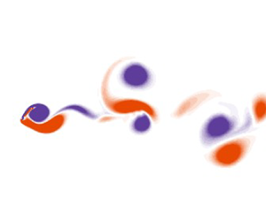
Figure 5. Progression of the shear-layer dominated states with increasing  $ {\kappa }$, for $\mu = 4.54$. (a–d) Undeformed equilibrium I; deformed equilibrium II; small-deflection flapping III; and small-amplitude flapping IIIA. Time histories of the angular displacement are shown for all examples; frequency spectra of this displacement are shown for the small-deflection and small-amplitude flapping states. Flow visualisation are instantaneous images of vorticity, with purple/orange contours representing negative/positive non-dimensional vorticity, $\varOmega = \omega D/U$ between levels of ${\pm }1$.
4.1.1. Undeformed equilibrium: state I
For very low  $ {\kappa }$, the rigid inverted flag remains completely stationary. The flow is dominated by a wake consisting of two long shear layers produced from the boundary layers on each side of the flag. Figure 5 shows an example of this flow and the associated time history of the angular displacement of the flag, $\theta$, which is zero throughout.
4.1.2. Deformed equilibrium: state II
As  $ {\kappa }$ is increased, the first bifurcation occurs with the rigid inverted flag deflecting steadily to one side. The wake flow structure is almost unaffected relative to state I, except for a slight asymmetry; see figure 5. A similar biased state has been observed for the flexible inverted flag at a similar Re (Gurugubelli & Jaiman Reference Gurugubelli and Jaiman2015; Ryu et al. Reference Ryu, Park, Kim and Sung2015; Goza et al. Reference Goza, Colonius and Sader2018).
The rigid inverted flag acts as a thin airfoil that is prone to divergence instability; similar to a flexible inverted flag (Sader et al. Reference Sader, Huertas-Cerdeira and Gharib2016b). We consider a generalisation of the rigid inverted flag by considering the pivot point to occur at the Cartesian position,  $x_0$, along the plate; $x_0 = -L$ is the leading edge of the plate, with $x_0 = 0$ being its trailing edge, as per figure 1. The resulting hydrodynamic torque per unit width, $\boldsymbol {M}_{hydro}$, experienced by the plate about its pivot point, $x_0$, is given by thin airfoil theory in the inviscid limit (Tchieu & Leonard Reference Tchieu and Leonard2011)
 \begin{equation} \boldsymbol{M}_{hydro} ={-} \tfrac{1}{2} \rho U^2 L^2 C_M \hat{\boldsymbol{z}}, \end{equation}
where  $\hat {\boldsymbol {z}}$ is the Cartesian basis vector in the $z$-direction (see figure 1), and the dimensionless torque coefficient is
 \begin{equation} C_M = 2 {\rm \pi}\theta \left(\frac{x_0}{L}+\frac{3}{4}\right). \end{equation}
Adding this torque per unit plate width to that produced by the torsional spring,  $\boldsymbol {M}_{spring} = k_\theta \hat {\boldsymbol {z}}$, at the pivot point, gives the critical dimensionless flow speed for a divergence (zero stiffness) instability
 \begin{equation} {\kappa}_{{critical}} = \frac{\rho U^2 L^2}{k_\theta} = \frac{1}{\rm \pi}\left(\frac{x_0}{L}+\frac{3}{4}\right)^{{-}1}, \end{equation}
establishing that a divergence instability occurs only if the pivot position satisfies
 \begin{equation} x_0 >{-}\frac{3 L}{4}, \end{equation}
i.e. the pivot position must be downstream from the quarter-chord position. This shows that a rigid conventional flag (with a pivot position at its leading edge,  $x_0 = -L$) cannot exhibit a divergence instability; it also cannot undergo coupled-mode flutter (at least due to coupling between structural modes) due to its single structural degree of freedom.
For the rigid inverted flag considered here, i.e.  $x_0 = 0$, (4.3) gives a divergence instability at
 \begin{equation} {\kappa}_{{critical}} = \frac{4}{3{\rm \pi}} \approx 0.424. \end{equation}
 The precise boundary between states I and II in the simulations is difficult to discern, but certainly occurs for  $\kappa > {\kappa }_{{critical}} \approx 0.424$. This critical (inviscid) value is indicated in figure 3 as a dashed vertical line. Finite Reynolds number is known to lower the lift experienced by a thin airfoil (Gurugubelli & Jaiman Reference Gurugubelli and Jaiman2015), which is consistent with this enhanced viscous value for $\kappa _{critical}$ in simulations. This observation suggests that the rigid inverted flag undergoes a divergence instability as the dimensionless flow speed, $\kappa$, is increased, following which (deflected) state II emerges and is observed for all angles, $\theta \lesssim 5.7^\circ$. This behaviour is similar to that observed for the flexible inverted flag, where a small-amplitude deflected equilibrium is observed for low flow speeds (Goza et al. Reference Goza, Colonius and Sader2018).
4.1.3. Small-amplitude simple flapping: state III
As the flow speed,  $\kappa$, is increased further, state II gives way to unsteady motion of the rigid inverted flag. Figure 5 shows such a ‘state III’ for a slightly larger value of $ {\kappa } = 0.713$ with respect to the case shown for state II ( $ {\kappa } = 0.675$). Very small-amplitude periodic oscillations are observed to occur in state III about the mean deflected position; the flag does not cross its zero deflection equilibrium position, $\theta = 0$. For the flexible inverted flag, Goza et al. (Reference Goza, Colonius and Sader2018) showed that this state arises from a bifurcation of the small-amplitude deformed equilibrium.
Figure 5 shows that the wake of state III is still dominated by long shear layers, but these layers start to break up downstream. This state bears a striking resemblance to small-amplitude stall flutter (Razak, Andrianne & Dimitriadis Reference Razak, Andrianne and Dimitriadis2011). Physically, such an instability occurs via the following mechanism:
(i) Initially, the deflected flag generates enough lift to deflect it beyond the angle at which the flow separates from its leading edge and upper surface.
(ii) This flow separation causes a loss of lift, which leads to the flag angle decreasing.
(iii) The decreased angle allows the flow to reattach to the flag surface.
(iv) The flag returns to its original position and the process repeats.
Because the flag angle is always small, the separated flow does not roll up into a distinct vortex but merely deforms the shear layers in the wake.
While the explanation of the observed behaviour in terms of stall flutter is not definitive, it appears that small-amplitude stall flutter could also describe the observed small-amplitude periodic oscillation in the flexible inverted flag (Goza et al. Reference Goza, Colonius and Sader2018), discussed above. Note the similarity in the Strouhal numbers exhibited by the rigid and flexible inverted flags in this regime: for a light flexible inverted flag, Goza et al. (Reference Goza, Colonius and Sader2018) record a value of  $St \equiv fL/U \approx 0.1$, whereas the example shown in figure 5 for a light rigid inverted flag with $\mu = 4.54$ and $\kappa = 0.713$ gives $St \approx 0.09$.
4.1.4. Small-amplitude complex flapping: state IIIA
The presence of stall flutter is further supported by the following observation, where the dimensionless flow speed is slightly increased from  $ {\kappa } = 0.713$ (for state III) to $ {\kappa } = 0.733$. This also leads to small-amplitude flapping but now with a complex time series at significantly lower fundamental frequency, and around the zero deflected equilibrium, $\theta = 0$; see figure 5. The wake is again formed by two shear layers which are deformed/modulated by the flag motion. Strikingly, the frequency spectrum shows a primary oscillation frequency approximately one third that of state III. The complex and distorted time series of $\theta$, relative to state III (at $ {\kappa } = 0.713$), indicates the origin of this behaviour:
(i) Initially, there is one cycle of the stall flutter process, that increases the deflection angle then decreases it following separation. However, the maximum deflection angle exceeds that of state III which leads to a very slight overshoot past
$\theta = 0$.(ii) The flag then re-approaches
$\theta = 0$, which is unstable once the flow reattaches, because $\kappa$ exceeds that for divergence instability.(iii) The stall flutter cycle repeats, but now on the other side of
$\theta = 0$.


The first and third steps in this process are identical to that for state III, while the time series in figure 5 shows that the second step takes similar time. This explains the origin of the threefold decrease in the observed oscillation frequency relative to state III.
Other examples of this small-amplitude complex flapping state are observed for different mass ratios,  $\mu$ (data not shown). They contain slightly different frequency profiles and some exhibit oscillations about $\theta \neq 0$. However, all of this dynamics can be described by the above-mentioned stall flutter process. State IIIA, with its complex time series, has not been reported in previous studies of flexible inverted flags; it occurs over a very small range of $\kappa$.
The stability analysis of Goza et al. (Reference Goza, Colonius and Sader2018), for the flexible inverted flag, indicates that the small-deflection flapping state is a limit cycle oscillation that encircles the unstable equilibrium position. The numerical results here, for the rigid inverted flag, show that the oscillation amplitudes of states III and IIIA are similar. Moreover, states III and IIIA do not significantly alter the vorticity and wake structure near the body, with no coherent vortex shedding; see figure 5. Taken together, these facts suggest that state IIIA results from a heteroclinic connection between the two (now unstable) limit cycles on each side of  $\theta = 0$ for state III.
This conclusion is further supported by the results in figure 6, which gives the trajectories in  $(\theta, \dot {\theta })$ phase space, for $\kappa = 0.713$ (state III) and $\kappa = 0.733$ (state IIIA). Note that the deflection angle never crosses $\theta = 0$ for state III, while it overshoots $\theta = 0$ for state IIIA. Once the trajectory crosses $\theta = 0$, it is initially attracted into the limit cycle traced by state III (at very similar $\kappa$). The trajectory then spirals out, gradually diverging from the state III limit cycle and causing the angle to again cross $\theta = 0$ in the opposite direction. The same process is repeated on the other side, completing the heteroclinic cycle.

Figure 6. Phase portraits in the  $(\theta, \dot {\theta })$ space of the small-deflection flapping state III and the small-amplitude flapping state IIIA. Blue solid/dashed lines show limit cycles for the small-deflection flapping state deflected to the left/right, for $\mu = 4.54$ and $\kappa = 0.713$. The fine orange line is the cycle for the small-amplitude flapping state IIIA with a small increase in $ {\kappa }$, to $ {\kappa } = 0.733$. For the state IIIA case, when the angle crosses $\theta = 0$ (i.e. the flag overshoots the neutral position) a path is traced that spirals away from the limit cycle for the state III case, which causes the flag to overshoot in the other direction; the process repeats on the other side of the neutral position.
4.2. Flapping dynamics: periodic organising states
For the flexible inverted flag, Sader et al. (Reference Sader, Cossé, Kim, Fan and Gharib2016a) presented an argument for the appearance of large-amplitude flapping as a VIV, based on the framework that the flapping arises when there is a synchronisation between a preferred wake or vortex shedding frequency, and the natural structural frequency of the flag. We show here that the same concept of synchronisation and an interaction between time scales is useful in analysing the rigid inverted flag. We find no evidence that contradicts the theory that the large-amplitude flapping is a vortex-induced vibration, and we discuss the point of potential mechanisms in § 4.2.2.
4.2.1. Interaction between vortex shedding and flag natural frequencies
Knisely (Reference Knisely1990) studied vortex shedding by rigid flat plates and showed that the Strouhal number,  $St \equiv f_{vs}H/U \approx 0.17$, for all appreciable angles of attack $\phi$, where $f_{vs}$ is the vortex shedding frequency and $H$ is the projected frontal length. For the rigid inverted flag, this frontal length, $H$, is directly related to the plate length, $L$, and the amplitude of oscillation, $\theta$, via $H = 2L\sin \theta$. Therefore, the vortex shedding frequency normalised by the plate length can be estimated in the quasi-static limit, as $f_{vs}L/U \approx 0.085/\sin \theta$. Figure 3 shows that at the onset of large-amplitude flapping, the amplitude is $\theta \approx 45 {^\circ }$, which gives a normalised vortex shedding frequency $f_{vs}L/U \approx 0.12$. This frequency and its subharmonic are marked on the spectrograms of figure 3.
We now calculate an estimate for the natural flapping frequency for the rigid inverted flag. Its natural frequency in vacuo,  $f_N = 1/(2{\rm \pi} ) \sqrt {k_\theta /I}$, where $I$ is the moment of inertia per unit width of the flag, is not appropriate here due to the significant added mass (inertia) of the fluid. This added inertia, characterised by its moment per unit width, $I_a$, is proportional to that of a cylinder of fluid of radius, $L$, i.e. $I_{{cyl}}$, that is the potential volume swept by the flag, i.e.
 \begin{equation} I_a = c_I I_{{cyl}}, \end{equation}
where  $c_I$ is a dimensionless order-one coefficient. We can non-dimensionalise $I_{{cyl}}$ by the flag's moment of inertia, $I$, to obtain
 \begin{equation} \frac{I_{{cyl}}}{I} = \frac{\dfrac{1}{2}{\rm \pi}\rho L^4}{\dfrac{1}{3}\rho_s h L^3} = \frac{3}{2}{\rm \pi}\mu. \end{equation}
Combining (4.6) and (4.7) gives
 \begin{equation} I_a = \tfrac{3}{2}{\rm \pi} c_I \mu I, \end{equation}
which then leads to the corrected natural frequency of the rigid inverted flag
 \begin{equation} f_{N_{f}} = \frac{1}{2{\rm \pi}}\sqrt{\frac{k_\theta}{I+I_a}} = f_N\sqrt{\frac{1}{1+ \dfrac{3}{2} {\rm \pi}c_I \mu}}, \end{equation}
where  $c_I$ remains to be evaluated.
Note that this is essentially the same idea as that traditionally employed when calculating an added mass to analyse the VIV of circular cylinders (Gopalkrishnan Reference Gopalkrishnan1993; Khalak & Williamson Reference Khalak and Williamson1996; Govardhan & Williamson Reference Govardhan and Williamson2002). The ‘impulsive added mass’ – derived from the hydrodynamic force arising from impulsive motion of the body – can be calculated (Magnaudet Reference Magnaudet2011), and this has been done with some success for oscillating cylinders that are both externally controlled and undergoing VIV (Leonard & Roshko Reference Leonard and Roshko2001; Carberry, Sheridan & Rockwell Reference Carberry, Sheridan and Rockwell2005). An ‘apparent added mass’ could also be derived from all of the fluid force that is in phase with the acceleration, which will include the impulsive added mass plus a component due to the presence of vorticity. In the remainder of this section and Appendix B, we determine  $c_I$ both theoretically in the inviscid limit, and empirically by fitting to the simulation data thereby including the impact of viscosity and vorticity.
No impinging flow: we first consider the special case of no impinging flow and small-amplitude oscillation, which is amenable to both analytical and numerical evaluation. This provides a baseline for the effect of non-zero impinging flow. The evaluation is characterised in terms of the oscillatory Reynolds number
 \begin{equation} Re_{\omega} = \frac{\omega_{N_{f}}L^2}{\nu}, \end{equation}
where the angular frequency,  $\omega _{N_{f}}= 2{\rm \pi} f_{N_{f}}$. The case of inviscid flow, $Re_{\omega } \rightarrow \infty$, is calculated analytically in Appendix B and gives
 \begin{equation} c_I = \tfrac{9}{64} \approx 0.141. \end{equation}
 To evaluate  $c_I$ for finite $Re_{\omega }$, numerical simulations are performed using the immersed-boundary code for the flag with a very small initial displacement. The resulting damped oscillations or ‘ring down’ then provides access to the linear resonant frequency and hence $c_I$ (Chakraborty et al. Reference Chakraborty, Van Leeuwen, Pelton and Sader2013). These numerical results are reported in figure 22, showing that the effect of viscosity is to enhance the added mass (inertia) in the fluid, as expected.
Large-amplitude flapping: next, we consider the large-amplitude flapping dynamics of a rigid inverted flag, for which we determine  $c_I$ using (4.9) (Chakraborty et al. Reference Chakraborty, Van Leeuwen, Pelton and Sader2013); $f_{N_{f}}$ is taken to be the flapping frequency. Figure 3 shows that for the lighter flags ( $\mu = 2.27$ and $4.54$), large-amplitude flapping first occurs via a periodic state $ {P_{1}}$ that is synchronised with the vortex shedding frequency. Figure 7 gives $c_I$ for these cases as a function of the dimensionless flow speed, $\kappa$, and the oscillatory Reynolds number $Re_\omega$. The reported values of $c_I$ are an order-of-magnitude higher than for the case of no impinging flow (above), commensurate with substantial vortex shedding in the $ {P_{1}}$ state. Interestingly, $c_I$ is found to be a weak function of $\kappa$ which ranges from $c_I \approx 1.4$ at the onset of flapping down (lower $\kappa$) to $c_I \approx 1.2$ at the loss of stability of the periodic state (higher $\kappa$).

Figure 7. Added inertia coefficient,  $c_I$, defined in (4.9) as a function of (a) the dimensionless flow speed, $\kappa$, and (b) an oscillatory Reynolds number, $Re_{\omega }$, for the first periodic flapping state $ {P_{1}}$ identified for the two mass ratios, $\mu = 4.54$ ( $\bullet$, blue) and $\mu = 2.27$ ( $\bullet$, orange).
As a heuristic, we apply the value  $c_I \approx 1.4$ obtained near the onset of $ {P_{1}}$ flapping, to all flapping states to calculate a natural frequency $f_{N_f}$ accounting for the apparent added mass, shown as the solid curve in the spectrograms of figure 3. This provides reasonable agreement with the dominant frequencies in the numerically evaluated spectrograms, suggesting that inertia induced by vortex shedding is the primary mechanism controlling the flapping frequency, at the onset of flapping.
Finally, these estimates of vortex shedding frequency,  $f_{vs}$, and the natural frequency in fluid, $f_{N_{f}}$, provide a framework to understand the appearance of stable periodic states as a synchronisation between these two frequencies. The first periodic state may be expected when $f_{vs}$ and $f_{N_{f}}$ coincide. Figure 3 shows that the value of $ {\kappa }$ at which this coincidence occurs is quite close to the value at which the periodic state $ {P_{1}}$ occurs with the onset of large-amplitude flapping. However, for the heavier flag ( $\mu = 0.39$), $f_{vs} = f_{N_{f}}$ at a value of $ {\kappa }$ that is much lower, or equivalently, where the flag natural frequency is lower. In this case, the vortex shedding is too fast to match the preferred frequency of the flag, and the synchronisation to the periodic $ {P_{1}}$ does not occur. However, for this same heavier flag the value of $ {\kappa }$ at which the first subharmonic of the vortex shedding frequency coincides with the natural frequency ( $f_{vs}/2 = f_{N_{f}}$) is also lower, and a large range of $ {\kappa }$ is observed where the flow synchronises to a subharmonic state $ {P_{2}}$.
The various organising states can therefore be thought of as a synchronisation between the vortex shedding at a preferred frequency, and the oscillation of the plate at a corrected natural frequency. This natural frequency is that which incorporates the impact of the vortices on the apparent added mass. There is a type of ‘basin of attraction’ for this to occur, and the two frequencies need to be reasonably close for nonlinear effects to synchronise them. This suggests that even in situations where these synchronised states may not be stable, they can still play a role in the dynamics when the flow is chaotic. We show in § 4.3 that the chaotic oscillations are not the product of a single mechanism. There are multiple routes to chaos depending on the value of  $ {\kappa }$ and $\mu$, which are governed by the periodic states (albeit unstable) outlined above.
4.2.2. Discussion of potential mechanisms leading to large-amplitude flapping
The preceding discussion has presented a framework to understand the large-amplitude flapping dynamics in terms of synchronisation between the vortex shedding and the structural natural frequency, accounting for the apparent added mass of the fluid. While we have determined this added mass empirically, the data show that this simple approach is able to at least suggest the loss of stability of the  $ {P_{1}}$ state and the gain of stability of the $ {P_{2}}$ state with increasing plate mass or equivalently decreasing $\mu$, both of which are observed.
We note that similar ‘lock-ins’, or synchronisations have been observed for the flexible inverted flag, including the change from a harmonic to subharmonic synchronisation (Goza et al. Reference Goza, Colonius and Sader2018). Sader et al. (Reference Sader, Cossé, Kim, Fan and Gharib2016a) took this evidence – as well as the fact that large-amplitude flapping occurs at a value of  $ {\kappa }$ above that for divergence instability, such that the inverted flag already presents a sharp edge to the flow from which vortices can separate – as support for the hypothesis that the flapping is a VIV.
The loss of the harmonic synchronisation for heavy inverted flags has recently been studied experimentally and theoretically by Tavallaeinejad et al. (Reference Tavallaeinejad, Païdoussis, Legrand and Kheiri2020a,Reference Tavallaeinejad, Païdoussis, Salinas, Legrand, Kheiri and Botezb). Tavallaeinejad et al. (Reference Tavallaeinejad, Païdoussis, Legrand and Kheiri2020a) concluded that VIV cannot be the causal mechanism for the onset of instability of the undeflected equilibrium of the heavy flag because there does not appear to be a bifurcation from the equilibrium that could lead to VIV. Instead, Tavallaeinejad et al. (Reference Tavallaeinejad, Païdoussis, Salinas, Legrand, Kheiri and Botez2020b) attributed the instability leading to large-amplitude flapping of heavy flags to flutter-like modes, drawing an analogy to the coupled-mode flutter of conventional flags.
While the rigid and flexible inverted flag systems are not identical, the comparison of our rigid inverted flag data with those from the flexible inverted flag study of Goza et al. (Reference Goza, Colonius and Sader2018) indicates that their underlying fluid–structure mechanisms are similar – despite the rigid inverted flag possessing only one structural degree of freedom. That is, the mechanism of excitation for the rigid inverted flag cannot be coupled-mode flutter, at least not a flutter driven by the coupling of structural modes of the flag.
However, this does not rule out the idea that the large-amplitude flapping is a coupled-mode or movement-induced excitation (Naudascher & Rockwell Reference Naudascher and Rockwell1994; Païdoussis Reference Païdoussis2014) in the broader sense. Indeed, de Langre (Reference de Langre2006) produced a low-order model for the VIV of a circular cylinder, where the single degree-of-freedom structure was coupled to a van der Pol oscillator modelling the wake dynamics. This model reproduced the stability characteristics of classic coupled-mode flutter, where the coupling was between the structural mode and a wake mode. Further, it has been shown that ‘vortex-induced’ vibrations can occur for the classic system displaying VIV – the flow past an elastically mounted cylinder constrained to oscillate in the transverse direction – even when the flow past a fixed cylinder is completely steady, i.e. at Reynolds numbers  ${\textit {Re}} < 47$ (Dušek, Le Gal & Fraunié Reference Dušek, Le Gal and Fraunié1994). Experiments (Buffoni Reference Buffoni2003), global stability analysis (Navrose & Mittal Reference Navrose and Mittal2016) and a model based on an impedance criterion (Sabino et al. Reference Sabino, Fabre, Leontini and Lo Jacono2020) have all shown this ‘subcritical’ VIV. In this case, VIV must be thought of as a movement-induced excitation; the oscillation of the flow and structure are intrinsically coupled. This is contrasted against the view that VIV is an instability-induced excitation (Naudascher & Rockwell Reference Naudascher and Rockwell1994; Païdoussis Reference Païdoussis2014), where the presence of vortices (even when the structure is completely stationary) is what causes the onset of structural motion.
We have not observed anything in the rigid inverted flag problem that contradicts the argument that the large-amplitude flapping is a VIV – in fact, the synchronisation characteristics across both light and heavy flags and the flow visualisation of the synchronised modes adds evidence for it. The single degree of freedom definitively rules out coupling between structural modes, as occurs in a conventional elastic flag (which is free at its trailing edge), leading to instability.
However, we cannot conclude definitively that VIV – interpreted as either a movement-induced excitation stemming from an instability of the undeflected equilibrium, or as an instability-induced excitation caused by vortices shed from the inverted flag that is deflected by other instabilities including divergence – is at the inception of the flapping. A full global stability analysis of the rigid inverted flag – which may be simpler to interpret than a similar analysis of the flexible inverted flag – is required to definitively settle the question of the mechanism of inception which we suggest as a future research direction.
In the following sections, we focus on the periodic states that arise due to synchronisation, organised in order of increasing  $ {\kappa }$.
4.2.3. Synchronised state: $ {P_{1}}$

Figure 8 presents data for the first organising periodic (synchronised) state,  $ {P_{1}}$, with $ {\kappa } = 0.835$ and $\mu = 4.54$. The time history and frequency spectrum both show clear periodicity, with an amplitude of $ {\theta _{{max}}} \approx 45 {^\circ }$. Vortex shedding is also periodic with the same frequency as the flag oscillation. The wake structure is reasonably complex with the interaction of vortices generated from the leading and trailing edge of the flag. Goza et al. (Reference Goza, Colonius and Sader2018) identified a synchronised state as the first sub-regime of their mode IV for the flexible inverted flag. State $ {P_{1}}$ matches the ‘VIV mode’ identified by Goza et al. (Reference Goza, Colonius and Sader2018); we have renamed it to fit an overall classification of a more extensive collection of states.

Figure 8. Synchronised state  $ {P_{1}}$: (a) time history of the angular displacement; (b) frequency spectrum of the angular displacement; and (c) an image of the vorticity field at $\tau = 350$, for $ {\kappa } = 0.835$ and $\mu = 4.54$. Black dashed line marks the nominal Strouhal frequency $f = 0.12$. Orange dashed line marks the first subharmonic, $f = 0.06$.
Vortex formation process: the far wake consists of four distinct vortices per cycle: a pair of oppositely signed strong vortices in the middle of the wake and a weaker vortex of each sign off to each side. The strong vortices in the middle are organised in an inverted Kármán configuration, i.e. their sense of rotation induces a jet, not a wake. However, the structure nearer the body shows that six unique vortices are shed per oscillation cycle, or three per half-cycle. Two of these vortices are formed as a pair due to motion of the leading edge of the flag, as it accelerates from close to its maximum displacement back towards its neutral position; they are shed close to the point where the flag is pointing straight into the flow, both ejected from the trailing edge. The pair of vortices are annotated as  $L_{1}^-$ and $L_{1}^+$ in figure 8: $L_{1}^-$ is the leading-edge vortex formed by the separated flow at the leading edge as it accelerated down; $L_{1}^+$ is a vortex of opposite sign formed from the vorticity on the top of the flag that is induced by the formation of the separated leading-edge vortex $L_{1}^-$. The third vortex, $T_{1}^-$, is shed from the trailing edge when the flag is close to its maximum anti-clockwise displacement presenting an upwards ramp to the flow. This process occurs in reverse as the flag accelerates up; the three vortices, $L_{2}^+$, $L_{2}^-$ and $T_{2}^+$, shed during the previous upward-accelerating half-cycle are also annotated on figure 8. The stronger vortex of the leading edge pair eventually wraps the weaker vortex and annihilates it, forming a single large central wake vortex, whereas the trailing-edge vortex becomes the weaker vortex off to the side of the wake.
4.2.4. Asymmetric subharmonic state: $ {P_{2_{A}}}$

The second of the organising states is a large-amplitude state which is asymmetric in terms of the lift and mean displacement of the flag. An example of this subharmonic state is shown in figure 9, for  $ {\kappa } = 1.013$ and $\mu = 4.54$. Its periodicity is clear from the displacement time history, and its subharmonic nature is evident by the significant frequency component at half of the primary frequency.

Figure 9. Asymmetric state  $ {P_{2_{A}}}$: (a) time history of the angular displacement; (b) frequency spectrum of the angular displacement; and (c) an image of the vorticity field at $\tau = 300$, for $ {\kappa } = 1.013$ and $\mu = 4.54$. Black dashed line marks the nominal Strouhal frequency, $f = 0.12$. Orange dashed line marks the first subharmonic, $f = 0.06$.
Vortex formation process: figure 10 shows a sequence of images over one cycle of oscillation, along with the time history of the flag displacement over two cycles of oscillation. The first two images show that as the flag accelerates from its maximum clockwise displacement to its neutral position, a large negative leading-edge vortex is formed. This pairs with the vortex formed by the positive vorticity induced on the top surface of the flag, forming the first leading-edge pair ( $L_-^1, L_+^1$). The third and fourth images of figure 10 show that as the flag accelerates from its maximum anti-clockwise displacement towards its neutral position, a similar process occurs but with reversed signs on the vortices, forming the second leading-edge pair ( $L_+^2, L_-^2$). However, as the flag approaches its neutral position it does not cross the centreline, and it instead stagnates at a small negative angle. During a period of stagnation (see fifth image), a small pair of vortices are shed into the wake ( $W_+, W_-$) – essentially from the trailing edge of the flag – and the flag deflects in the anti-clockwise direction again. After this anti-clockwise deflection, the flag then again accelerates towards its neutral position as shown in the sixth image, and during this acceleration a final pair of leading-edge vortices are formed and shed ( $L_+^3, L_-^3$). The flag motion continues past the neutral position to its maximum clockwise deflection, and the cycle repeats.

Figure 10. Asymmetric state  $ {P_{2_{A}}}$: snapshots of vorticity in the near wake, with the time history of angular displacement of the flag. Circles on the time history coincide with the instants shown in the images. One leading-edge pair of vortices, ( $L_-^1, L_+^1$), is shed from the top side of the flag, while two leading-edge pairs, ( $L_-^2, L_+^2$), ( $L_-^3, L_+^3$), are shed from the bottom side, with a wake pair, ( $W_+, W_-$), shed in between these two leading-edge pairs. The example shown is the same case as figure 9, i.e. $ {\kappa } = 1.013$ and $\mu = 4.54$.
4.2.5. Symmetric subharmonic state: $ {P_{2}}$

The third organising state is a subharmonic state, with two cycles of vortex shedding occurring over a single cycle of the flag motion. Figure 11 shows an example case of this state for  $ {\kappa } = 1.572$ and $\mu = 0.39$, which is only stable at this lower $\mu$. The subharmonic nature of the state is clear from the spectrum in figure 11: the primary peak is aligned with $f_{vs}/2$. Its amplitude is very large, with the angle of displacement exceeding $90 {^\circ }$, so that the flag goes past a vertical orientation; see flow visualisation in figure 12. The flag spends a large portion of the cycle approximately normal to the flow, which dictates the vortex shedding and formation.

Figure 11. Symmetric subharmonic state  $ {P_{2}}$: (a) time history of the angular displacement; (b) frequency spectrum of the angular displacement; and (c) an image of the vorticity field at $\tau = 300$, for the case $ {\kappa } = 1.572$ and $\mu = 0.39$. Black dashed line marks the nominal Strouhal frequency, $f = 0.12$. Orange dashed line marks the first subharmonic, $f = 0.06$.

Figure 12. Close-up images of the symmetric subharmonic state  $ {P_{2}}$ over a half-cycle of oscillation. (a) At maximum displacement, $\theta = 98 {^\circ }$; (b) during the acceleration phase, with the flag at $\theta = 61 {^\circ }$; (c) at the neutral position, pointing almost straight into the flow $\theta = 5 {^\circ }$; (d) during the deceleration phase, $\theta = -52 {^\circ }$; and (e) at maximum displacement pointing downward, $\theta = -98 {^\circ }$. Three main vortices – a Kármán wake pair, ( $k_-$ and $k_+$), and a leading-edge vortex, ( $L_-$) – dominate the dynamics, with a smaller vortex induced by the leading-edge vortex of opposite sign, ( $L_+$), and an elongated trailing-edge vortex, $T_-$, playing a secondary role.
Vortex formation process: vortex formation and shedding is dominated by two processes: (i) Kármán-like vortex shedding when the flag is approximately normal to the flow, resulting in a vortex being shed from the leading edge, then one from the trailing edge; and (ii) formation of a leading-edge vortex during the accelerating phase of the motion. Figure 12 shows close-up images of the flow over a half-cycle of oscillation for the same case as figure 11.
The first image is at a phase of the flag motion that is close to its maximum clockwise displacement, i.e.  $\theta \approx 98 {^\circ }$, and therefore is almost normal to the flow. At this phase, vortices roll up from each side of the normal plate, reminiscent of Kármán vortex shedding. The first image shows the formation of the first of the Kármán vortices of a pair from the leading edge of the plate, labelled $k_-$.
The second image shows the flag at  $\theta \approx 61 {^\circ }$, during its anti-clockwise motion towards its neutral position. The second Kármán vortex forming from the trailing edge is clear (labelled $k_+$). Both the Kármán wake vortices $k_-$ and $k_+$ have grown, and there is also a large amount of negative vorticity generated from the accelerating leading edge. This is still feeding the negative Kármán vortex, but is also starting to roll up into a defined leading-edge vortex as described in the third image.
The third image shows the flag at close to its neutral position ( $\theta \approx 5 {^\circ }$), pointing almost straight into the oncoming flow. The negative Kármán vortex, $k_-$, has been shed and the positive Kármán vortex, $k_+$, is about to detach with only a thin layer of positive vorticity from the lower side of the flag still feeding it. The negative vorticity previously feeding $k_-$ has rolled up into a leading edge vortex, $L_-$. This vortex, $L_-$, has progressed to the trailing edge and its presence above the flag has induced positive vorticity on the upper side of the flag.
The fourth image shows the flag at  $\theta \approx -52 {^\circ }$. The negative Kármán vortex, $k_-$, has been shed while the positive Kármán vortex, $k_+$, and the negative leading-edge vortex, $L_-$, have been ejected from the trailing edge as a dipole pair. The detachment and shedding of the negative leading-edge vortex, $L_-$, and the fact that the flag top surface when angled down generates a favourable pressure gradient, induces the flow to reattach. Consequently, the positive vorticity that had been formed on the top surface rolls up into a small positive vortex, $L_+$, trailing the larger dipole pair. The negative vorticity formed in the boundary layer on the top surface of the flag also starts to roll up into a vortex labelled, $T_-$, as it separates from the trailing edge. These small positive and negative vortices are secondary to the main Kármán vortices, $k_-$ and $k_+$, and the leading-edge vortex, $L_-$.
The fifth and final image shows the flag at close to its maximum anti-clockwise displacement. The vortex structure is a mirror image of the structure at maximum clockwise displacement.
4.2.6. Deflected state: $ {D}$

The final state is the deflected state,  $ {D}$, shown in figure 13 for $ {\kappa } = 2.913$ and $\mu = 4.54$. This is almost stationary in a laid-over configuration, where the hydrodynamic force experienced by the flag is balanced by the torsional spring. The wake structure and vortex shedding frequency is similar to that of a stationary flat plate. This state coincides with mode VI for the flexible inverted flag identified by Goza et al. (Reference Goza, Colonius and Sader2018). While vortex shedding from state $ {D}$ is periodic in the near wake, there is a secondary instability that leads to the two rows of Kármán vortices breaking down into a lower frequency, longer wavelength configuration. In figure 13, this occurs around $10L$ downstream. This phenomenon has been documented in a number of bluff-body wakes that form this two-row vortex structure, e.g. see Hosseini, Griffith & Leontini (Reference Hosseini, Griffith and Leontini2021), and is associated with an absolute instability of the mean wake profile.

Figure 13. Deflected state  $ {D}$: (a) time history of the angular displacement; (b) frequency spectrum of the angular displacement; and (c) an image of the vorticity field at $\tau = 342$, for the case $ {\kappa } = 2.815$ and $\mu = 4.54$. Black dashed line marks the nominal Strouhal frequency $f = 0.12$. Orange dashed line marks the first subharmonic $f = 0.06$.
4.3. Flapping: chaotic states observed for all cases
The previous sections describe the various periodic states that can be observed. In this section, we describe the routes to chaos that occur via the loss of stability, and the nonlinear interaction of, these periodic states. These routes to chaos occur for all values of the mass ratio,  $\mu$, tested. These chaotic states are listed in order of increasing $ {\kappa }$. The examples shown are for $\mu = 2.27$, and the values of $ {\kappa }$ are marked on figure 4(b). Section 4.4 shows a further route that only appears for the lower- $\mu$ flags.
4.3.1. Instability of the synchronised state $ {P_{1}}$: type I intermittency

The first route to chaos that we examine is the loss of stability of state  $ {P_{1}}$. Figure 14 shows time history of the angular displacement for (i) a stable $ {P_{1}}$ case, and (ii) an unstable case with a slightly higher value of $ {\kappa }$. The latter case shows almost periodic oscillations, interspersed with high-amplitude bursts. Both cases are also plotted in the $(\theta, \dot {\theta })$ phase space which shows a limit cycle for the stable case that appears to act as an attractor; orbits of the unstable case are close to this attractor for a number of cycles (with almost periodic oscillations), but eventually spiral away (high-amplitude bursts), before returning back towards the attractor. This ‘type I intermittency’ (Pomeau & Manneville Reference Pomeau and Manneville1980) has been demonstrated in a number of dynamical systems and discrete maps.

Figure 14. Instability of  $ {P_{1}}$ leading to type I intermittency. (a,b) Show time histories of flag angular displacement for mass ratio, $\mu = 2.27$, with $\kappa = 0.810$ ((a), blue) and $\kappa = 0.885$ ((b), orange). These represent a stable $ {P_{1}}$ case, and an unstable case. The same cases are plotted in the $(\theta, \dot {\theta })$ plane on the right; the stable case with a bold blue line and the unstable case with the finer orange line. This plot shows the limit cycle for the stable case, with the unstable case orbiting close to this limit cycle for many periods before spiralling away, then collapsing back to the unstable limit cycle.
We note here that this route to chaos only relies on a periodic solution existing at nearby parameter values. The periodic solution itself may never be observed. We highlight this point as this type I intermittency occurs for both higher and low values of  $\mu$, while a stable periodic solution (state $ {P_{1}}$) is only observed for the higher- $\mu$ cases. The fact that $ {P_{1}}$ is not observed for the lower- $\mu$ case, $\mu = 0.39$, does not preclude this route to chaos.
4.3.2. Instability of state $ {P_{2_{A}}}$ generates heteroclinic-like orbits

The second route to chaos is organised around state  $ {P_{2_{A}}}$. Because this state is asymmetric, it can be biased to either positive or negative angular displacements. This presents two attracting states, either of which can be reached depending on the initial conditions if the state is stable. If this $ {P_{2_{A}}}$ state is unstable, it presents two unstable limit cycles in the $(\theta, \dot {\theta })$ phase space. The flag dynamics may visit each of these cycles for some time, before diverging and potentially settling towards the other cycle. After some time the dynamics will diverge from this cycle, and settle again towards the original cycle, where the process can repeat. This is similar to a heteroclinic cycle – the cyclic nature of the dynamics is driven by attraction to one state, but then repulsion in at least one direction in phase space. This direction of repulsion from one state drives the dynamics towards the second state, which itself is unstable – which drives the dynamics back towards the original state.
Figure 15 shows an example of this process. In panel (a), the two possible limit cycles in the  $(\theta,\dot {\theta })$ phase space are shown for a stable $ {P_{2_{A}}}$ . In panel (b), the trajectory traced by a case at a slightly higher value of $ {\kappa }$, which is unstable, is given. This clearly shows that the unstable orbit spends time cycling near an orbit of the $ {P_{2_{A}}}$ state, before spiralling away and being attracted toward the orbit of the $ {P_{2_{A}}}$ state biased to the other side. The cycle is not perfect, leading to a chaotic trajectory organised around the two manifestations of the $ {P_{2_{A}}}$ state.

Figure 15. Phase portraits in the  $(\theta, \dot {\theta })$ plane, demonstrating heteroclinic-like mode competition between the two manifestations of the asymmetric state $ {P_{2_{A}}}$. (a) Shows the trajectory for state $ {P_{2_{A}}}$, at $\mu = 2.27$ and $\kappa = 0.996$. Solid/dashed line represents the state biased to the left/right. (b) Shows the trajectory for a case at a very slightly higher, $\kappa = 1.013$. The image shows that the dynamics spends time near one orbit before losing stability and spiralling to the orbit biased to the other side.
4.3.3. Mode competition between states $ {P_{2_{A}}}$ and $ {P_{2}}$


The third route to chaos is apparent mode competition between states  $ {P_{2_{A}}}$ and $ {P_{2}}$. Similar to the other states, this is demonstrated by trajectories in the $(\theta,\dot {\theta })$ phase space. Figure 16 shows (left to right) (i) the trajectories of the two possible, stable $ {P_{2_{A}}}$ states at $\mu = 2.27$ and $ {\kappa } = 0.996$, then (ii) the cycle for the stable $ {P_{2}}$ state (albeit at a lower value of $\mu = 0.39$), followed by (iii) the chaotic trajectory at $\mu = 2.27$ and $ {\kappa } = 1.822$.

Figure 16. Phase portraits in the  $(\theta, \dot {\theta })$ plane illustrating mode competition between organising states $ {P_{2_{A}}}$ and $ {P_{2}}$. (a) The trajectories for the stable $ {P_{2_{A}}}$ state, at $\mu = 2.27$ and $\kappa = 0.996$. Solid/dashed line represents the state biased to the left/right. (b) The trajectory for the stable $ {P_{2}}$ state, at $\mu = 0.39$ and $\kappa = 1.572$. (c) The trajectory for the chaotic oscillation, at $\mu = 2.27$ and $\kappa = 1.822$; the chaotic trajectory spends periods orbiting near each of the organising states.
The  $ {P_{2}}$ state is not stable for higher- $\mu$ flags, and this is why the example cycle shown in figure 16 is from the lower- $\mu$ flag. Note, however, that the chaotic trajectory does seem to orbit near this example cycle, providing evidence that the $ {P_{2}}$ state is still playing a role in organising the dynamics for the higher- $\mu$ flags.
4.3.4. Mode competition between states $ {P_{2}}$ and $ {D}$


The fourth route to chaos is apparent mode competition between the unstable  $ {P_{2}}$ state and the two manifestations of the deflected state $ {D}$ (deflected either to positive or negative angular displacement). Figure 17 gives the trajectory of an example case compared with stable examples of the two organising states involved. The range of $\dot {\theta }$ covered by the chaotic trajectory is smaller than that for the example where $ {P_{2_{A}}}$ plays a role (figure 16). Moreover, a number of small loops appear that gradually spiral out near the extremities of the range of $\theta$ covered. This shows that the flag spends long portions of time near the deflected $ {D}$ state, which eventually loses stability, causing the flag to execute oscillations similar to the subharmonic $ {P_{2}}$ state, before settling towards the $ {D}$ state again, possibly biased to the other side.

Figure 17. Phase portraits in the  $(\theta, \dot {\theta })$ plane illustrating mode competition between organising states $ {P_{2}}$ and $ {D}$. (a) The trajectory for the stable $ {P_{2}}$ state, at $\mu = 0.39$ and $\kappa = 1.572$. (b) The trajectory for the stable $ {D}$ state, at $\mu = 2.27$ and $\kappa = 2.545$. Solid/dashed line represents the state biased to the left/right. (c) The trajectory for the chaotic oscillation, at $\mu = 2.27$ and $\kappa = 2.169$; the chaotic trajectory spends periods orbiting near each of the organising states.
4.3.5. Instability of the deflected state $ {D}$

The fifth and last route to chaos found for all flags is mode competition between the regions of the deflected state  $ {D}$, i.e. positive and negative angular displacement. Figure 18 gives the trajectory of an example case, along with the two stable limit cycles representing $ {D}$. This shows that the trajectory is dominated by loops that orbit near one of the $ {D}$ cycles, that slowly spiral out. Physically, this represents the flag being deflected almost normal to the flow and exhibiting small, but growing oscillations. Eventually these oscillations become so large that they cause the flag to overshoot the centreline of the flow, causing it to be deflected to the other side, where this cycle again repeats.

Figure 18. Phase portraits in the  $(\theta, \dot {\theta })$ plane illustrating mode competition between the two possible manifestations of organising state $ {D}$. (a) Shows the trajectory for the stable $ {D}$ state, at $\mu = 2.27$ and $\kappa = 2.545$. Solid/dashed line represents the state biased to the left/right. (b) Shows the trajectory for the chaotic oscillation, at $\mu = 2.27$ and $\kappa = 2.291$; the chaotic trajectory spends periods orbiting near each of the examples of state $ {D}$, before flipping to the other.
This final route to chaos appears to be the state hypothesised by Goza et al. (Reference Goza, Colonius and Sader2018) to drive the chaotic oscillations in the flexible inverted flag. Whether the other routes to chaos identified above are present for the flexible inverted flag remains an open question.
4.3.6. Development of chaos across the flapping regime for higher $\mu$

The changing nature of the chaotic dynamics is further investigated in figure 19, which shows the time histories of the angular displacement for increasing  $ {\kappa }$ with $\mu = 2.27$.

Figure 19. Development of the time history of oscillation with increasing  $ {\kappa }$, for $\mu = 2.27$ in the large-amplitude flapping range. For low $ {\kappa }$ (e.g. $ {\kappa } = 1.131$), the flag oscillates for long epochs in a state similar to $ {P_{1}}$, interspersed with intermittent losses of stability. For slightly higher $ {\kappa }$ (e.g. $ {\kappa } = 1.312$), there are epochs of oscillation similar to $ {P_{2_{A}}}$, first biased to one side then the other. Higher $ {\kappa }$ again (e.g. $ {\kappa } = 1.506$) shows intermittent switching between epochs similar to $ {P_{2_{A}}}$ and $ {P_{2}}$. Higher $ {\kappa }$ again (e.g. $ {\kappa } = 1.822$) shows intermittent switching between epochs similar to $ {P_{2}}$ and the deflected state D. Finally for the highest $ {\kappa }$ shown, the dynamics settles to a stable deflected state D periodic oscillation.
For the smallest flow speeds, i.e.  $ {\kappa } < 1.2$, there are reasonably long epochs of time where the flag oscillates in a state similar to the periodic state $ {P_{1}}$, interspersed amongst intermittent epochs of disordered oscillations. This is seen in figure 19 for $ {\kappa } = 1.131$ – there is a long epoch, $170 < \tau < 250$, where the flag oscillates almost periodically, but the oscillations either side of this epoch fluctuate in amplitude and frequency. This is another example of the first route to chaos shown in figure 14.
Slightly increasing  $ {\kappa }$ sees the flag switch between two types of epochs: (i) the flag oscillates in a state similar to the periodic but asymmetric state $ {P_{2_{A}}}$ biased to one side, and (ii) the same state biased to the other side. See the example for $ {\kappa } = 1.312$ in figure 19, which shows that there are a number of cycles with the flag biased to negative angular displacement over $220 < \tau < 240$, and a cycle biased to positive angular displacement over $270 < \tau < 285$. This is an example of the second route to chaos illustrated in figure 15.
Increasing  $ {\kappa }$ further leads to epochs similar to the asymmetric state $ {P_{2_{A}}}$, interspersed with epochs reminiscent of the subharmonic state $ {P_{2}}$. See the example for $ {\kappa } = 1.407$ in figure 19 which shows chaos via mode competition between states $ {P_{2_{A}}}$ and $ {P_{2}}$ – the third route to chaos – as outlined in figure 16.
A further increase in  $ {\kappa }$ produces intermittent switching between the subharmonic state $ {P_{2}}$ and oscillations near the periodic deflected state $ {D}$. See the examples in figure 19 for $1.713 \leq {\kappa } \leq 1.934$, which also show that as $ {\kappa }$ is increased, the duration of the epochs spent in the subharmonic state $ {P_{2}}$ decreases while epochs near the deflected state $ {D}$ become more dominant. This dynamics corresponds to mode competition between states $ {P_{2}}$ and ${ {D}}$ – the fourth route to chaos – as per figure 17.
Larger values of  $\kappa$ again generate long epochs where the dynamics produces oscillations near the periodic deflected state $ {D}$ biased to one side, interspersed with epochs of the same state biased to the other side. This is shown in figure 19 for cases in the range $2.050 \leq {\kappa } \leq 2.291$. The chaotic motion cycles between the two manifestations of the deflected state $ {D}$, as outlined in figure 18 – the fifth route to chaos.
Finally, for the highest values of  $ {\kappa }$, the flag oscillations settle to the periodic deflected state $ {D}$, as shown for $ {\kappa } = 2.545$ in figure 19.
4.4. Flapping: chaotic states for the heaviest flag
The general picture of the development of chaos for the heaviest flag studied, i.e.  $\mu = 0.39$, is similar to the lighter flags as described in § 4.3. However, there is one important difference that we highlight here.
The spatio-temporally symmetric subharmonic state,  $ {P_{2}}$, is not found in a stable configuration for the two lighter flags, but occupies a reasonably large range of $ {\kappa }$ for the heaviest flag; see figures 3 and 4. This feature splits the $\kappa$-ranges where chaos via a heteroclinic-like cycle between the two manifestations of state $ {P_{2_{A}}}$ occurs, and where a cycle between the two manifestations of the deflected state $ {D}$ results. For the lighter flags, this same range is occupied by chaos via mode competition between states $ {P_{2_{A}}}$ and $ {P_{2}}$.
We propose that stabilisation of the subharmonic state  $ {P_{2}}$ presents another potential route to chaos via the interaction and instability of a series of states of increasing period, i.e. mode locking. Figure 20 gives time histories for increasing $ {\kappa }$, starting from a stable $ {P_{2}}$ case for $ {\kappa } = 1.659$. Increasing to $ {\kappa } = 1.747$ produces an extra ‘bump’ in each oscillation, and an apparent doubling of the oscillation period. As shown in figure 12, state $ {P_{2}}$ is formed via a cycle of Kármán-like shedding while the flag is oriented around $90 {^\circ }$. The flag then swings to the other side which is also followed by a cycle of Kármán-like shedding. The extra bump in each oscillation is due to a second cycle of vortex shedding, which occurs for the slightly reduced stiffness or increased $ {\kappa }$. Further slight reductions in stiffness (or increased $ {\kappa }$) allow for more Kármán cycles on each side, and a subsequent increase in the oscillation period.

Figure 20. Time histories of the oscillation for the heaviest flag,  $\mu = 0.39$, for increasing values of the dimensionless flow speed, $ {\kappa }$, displayed left to right, top to bottom. As $ {\kappa }$ is increased, evidence of states of oscillation with increasing numbers of vortex shedding cycles (for each half-oscillation cycle) is found – indicative of mode locking – until the period becomes so long that the flag remains on one side of the wake. Orange shaded regions mark epochs of possible mode locked oscillation, the number annotated in these regions indicates the number of vortex shedding periods per half-cycle. The first value of $ {\kappa } = 1.659$ corresponds to the stable state $ {P_{2}}$, the last value of $ {\kappa } = 2.326$ to the stable state $ {D}$.
Figure 20 shows that with increasing  $ {\kappa }$, there are epochs of oscillation with increasing numbers of vortex shedding cycles. This is consistent with mode locking. Weakly nonlinear systems that are periodically driven will often ‘lock’ to that period, or an integer multiple of that period. This is likely to occur when the driving period is close to a natural frequency, or a sub-harmonic of the natural frequency of the system. This means that as the driving frequency (or the ratio of the driving frequency to the natural frequency) is varied, ranges of the driving frequency can occur where the dynamics is synchronised and periodic, which are interspersed among ranges where the dynamics is more complex. In the circle map, these synchronised ranges are referred to as Arnold tongues (Arnol $\acute{{\rm d}}$ Reference Arnol1965). The width of the Arnold tongues are typically proportional to the ratio between the driving frequency and the natural frequency being synchronised, i.e. there is a wider locking range when the driving frequency is close to the natural frequency than when the driving frequency is close to the first subharmonic.
This feature is consistent with the observations of this study, if the rigid inverted flag is considered as a weakly nonlinear oscillator driven by vortex shedding. Namely, there is:
(i) A reasonably wide range of synchronisation to the state, where one vortex shedding cycle occurs on each side (the stable state
$ {P_{2}}$).(ii) A much smaller range of synchronisation, where two shedding cycles occur on each side.
(iii) Subsequently ever smaller ranges, where larger numbers of vortex shedding cycles occur, interspersed with ranges of more complex oscillations.

This is consistent with our inability to observe the lower frequency subharmonics (those with more vortex shedding cycles per half-cycle of oscillation) in a ‘pure’ stable state – the frequency range or  $ {\kappa }$ for which they are stable becomes vanishingly small. Similar mode locking cascades have been observed in the somewhat-related flows of forced cylinder wakes (Leontini, Lo Jacono & Thompson Reference Leontini, Lo Jacono and Thompson2011, Reference Leontini, Lo Jacono and Thompson2013) and the flow-induced vibration of square cross-sections undergoing transverse galloping (Zhao et al. Reference Zhao, Leontini, Lo Jacono and Sheridan2014).
5. Concluding remarks
The dynamics of a rigid and thin plate attached at its trailing edge to a torsional spring – a rigid inverted flag – has been investigated. This provides a practically realisable single degree-of-freedom mechanical analogue to the widely studied flexible inverted flag. The rigid inverted flag enables a focus on the fundamental interactions between the fluid and structure, by eliminating the complexity of the structural modes of the flexible inverted flag. The resulting structural dynamics is rich, and we have classified their equilibria, periodic and chaotic oscillations.
The dynamics of the rigid inverted flag was found to be strikingly similar to that of the flexible inverted flag. Elimination of any potential for coupling between structural modes in the former case – due to its single structural degree of freedom – establishes that such instabilities are not needed to generate the observed dynamics. We cannot, however, rule out coupling between the structural modes and modes of the flow leading to large-amplitude flapping dynamics via a movement-induced excitation.
The large-amplitude flapping dynamics of the rigid inverted flag is organised around a set of periodic states, which are a product of synchronisation between a nominal vortex shedding frequency and a natural frequency corrected to account for the apparent added mass. These states play a role as organising states during chaotic oscillations, even when they are not realisable as stable limit cycles. The fact that the stability of these periodic states can be associated with a synchronisation of vortex shedding and oscillation time scales, is consistent with large-amplitude flapping being a VIV.
Similar to the flexible inverted flag, the majority of the large-amplitude flapping states, particularly for lighter flags are chaotic. We have shown that this chaos is driven by competition between various states which are dependent on the dimensionless flow speed,  $ {\kappa }$, with mode locking also present for lower $\mu$.
The reported dynamics of the rigid inverted flag and its application, e.g. to energy harvesting, are yet to be realised experimentally.
Funding
J.S.L. acknowledges the provision of resources and services via competitive grant IZ4 from the National Computational Infrastructure (NCI) which is supported by the Australian Government. J.S.L. acknowledges the provision of computational resources at OzSTAR which is funded by Swinburne University of Technology and National Collaborative Research Infrastructure Strategy (NCRIS). J.E.S. acknowledges support from the Australian Research Council Centre of Excellence in Exciton Science (CE170100026) and the Australian Research Council grants scheme.
Declaration of interests
The authors report no conflict of interest.
Appendix A. Immersed-boundary method and convergence studies
Details of the immersed-boundary method used in this study are presented in this appendix.
A.1. Spatial discretisation
The fluid domain is spatially discretised using a Cartesian mesh with (2.1a,b) approximated using second-order central finite differences. The Cartesian mesh enables simple domain decomposition for efficient parallel computation. Solid body boundaries, i.e. the rigid inverted flag, are discretised using linear segments. The sharp-interface method is implemented by modifying the difference stencil for ‘ghost points’ in this Cartesian mesh, i.e. mesh points inside the solid body that have at least one neighbour point (a mesh point exactly adjacent) outside the body. On these points, an extrapolation scheme is used: a probe line is drawn from the ghost point to the closest point on the body surface; this probe line length is then doubled, so its end point is in the fluid and the closest point on the body surface is at its centre; the fluid field variables at the end of this line are obtained by interpolation from the surrounding mesh points; each interpolated value, and the desired boundary condition at the surface, are then used to linearly extrapolate a value at the ghost point.
This modification of the interpolation stencil produces the term,  $\boldsymbol {F}_b$, in the discretised version of (2.1a,b). This term is zero everywhere except at the ghost points. It maintains the overall second-order accuracy of the discretisation and ensures a sharp representation of the boundary. The present scheme closely follows Mittal et al. (Reference Mittal, Dong, Bozkurttas, Najjar, Vargas and von Loebbecke2008) and our particular implementation is detailed in Griffith & Leontini (Reference Griffith and Leontini2017).
A.2. Temporal discretisation
Equation (2.1a,b) is integrated in time using a two-way time-splitting scheme. A first substep equation is formed by integrating only the advection, diffusion and body acceleration terms – respectively, the first, third and fourth terms on the right-hand side of the momentum equation (2.1a,b) – to arrive at a velocity field at an intermediate time between the beginning and end of the time step. The advection term is solved using a second-order Adams–Bashforth scheme, the diffusion term using a second-order Crank–Nicolson scheme and the acceleration term via the extrapolation scheme outlined in § A.1. The resulting implicit equation is solved using Gauss–Jacobi iteration.
From this intermediate velocity field and the existing pressure field, (2.2) is integrated to update the body position using a Newmark- $\beta$ scheme. Any mesh points that emerge from the solid body into the fluid domain are assigned a value using an interpolation scheme, employing (i) the nearby mesh point values, and (ii) the boundary condition at the point on the body surface which is closest to the mesh point.
A second-order scheme is then employed for the pressure, which after enforcing mass conservation in (2.1a,b) produces a Poisson equation for the pressure correction. This Poisson equation is solved using a custom geometric multigrid method after employing a scheme to avoid odd–even decoupling or checker-boarding. A cut-cell scheme is employed to minimise the spurious force oscillations that can arise in sharp-interface immersed-boundary methods due to errors in the discrete conservation of mass (Seo & Mittal Reference Seo and Mittal2011). The eventual pressure correction is then used to update the velocity field from the intermediate time to the end of the time step.
A.3. Boundary and initial conditions
Standard external flow boundary conditions are used. For the velocity field, a free stream condition is imposed upstream ( $ {\boldsymbol {u}} = [U\ 0\ 0]^{T}$), while a zero-stress condition is applied at the transverse and downstream boundaries ( $\partial {\boldsymbol {u}}/\partial \boldsymbol {n} = 0$, where $\boldsymbol {n}$ is the normal vector). For the pressure, a zero gradient condition is used at the upstream and lateral boundaries ( $\partial p/\partial \boldsymbol {n} = 0$), and a Dirichlet condition ( $p = 0$) is applied downstream. At the immersed boundaries, a no-slip condition is imposed for the velocity such that the flow velocity matches the local surface velocity, and a zero gradient condition is used for the pressure ( $\partial p/\partial \boldsymbol {n} = 0$).
Two initial conditions are used. The first is to start the flow from rest. The second is to force the rigid inverted flag to perform two cycles of oscillations at a non-dimensional frequency of  $0.2$, and an amplitude of $0.25$ (or approximately $14.3 {^\circ }$), before allowing the flag to oscillate freely. This second initial condition is used in cases that would diverge when starting from rest due to numerical errors resolving the non-physical pressure field in the first time step. Cases that do not diverge are tested with both initial conditions, where the eventual saturated states are found to be insensitive to the choice of initial conditions.
A.4. Domain and mesh
The fluid domain used extended  $15L$ upstream, $36L$ downstream and $15L$ in the transverse direction from the trailing edge of the flag. The Cartesian mesh used for the fluid domain consisted of 1025 points in both the $x$ and $y$ directions, for a total of 1 050 625 points; the points are not equidistant, instead being concentrated in the area surrounding the flag. The mesh spacing used in a box $L\times L$ surrounding the flag is $\Delta x = \Delta y = L/256$. This guarantees at least 4 points exist across the plate thickness $h=0.022L$, regardless of the flag orientation. This ensures an accurate representation of the boundary of the flag at all times (using the extrapolation scheme for ghost point values) while also allowing for the use of a very thin flag. The mesh spacing from this box to the edge of the domain increases linearly in each direction.
A.5. Mesh resolution tests
Validity of the mesh is examined using a series of tests for  $\kappa = 1.045$ and $\mu = 2.27$. This case is chosen because it exhibits a complex dynamics and thus presents a hard test of the capacity of the simulation. Three configurations are tested by varying the mesh resolution and the plate thickness: (i) the configuration adopted in the rest of the study, $\Delta x = L/256$ and $h = (L/50)\times 1.1 = 0.022L$; (ii) a configuration with twice the plate thickness, $\Delta x = L/256$, and $h = 0.044L$; and (iii) a configuration with twice the plate thickness and twice the mesh spacing/half the resolution throughout the domain, $\Delta x = L/128$ and $h = 0.044L$. This allows the mesh resolution to be lowered while still retaining an accurate representation of the thicker plate in the immersed-boundary scheme.
Figure 21 shows phase space portraits in the  $(\theta, \dot {\theta })$ plane of these three configurations. The total time duration in these portraits is $250\tau$. All three cases display a similar dynamics, with their phase portraits producing two inner lobes surrounded by larger orbits that are bounded, but not repeating. Comparing the first two cases – same mesh resolution but different plate thickness – shows that their dynamics is reasonably insensitive to the plate thickness. For the second two cases – same plate thickness but different mesh resolution – their dynamics is also reasonably insensitive to the mesh spacing.

Figure 21. Resolution test results: phase portraits of plate angular frequency,  $\dot {\theta }$, as a function of $\theta$, for $ {\kappa } = 1.045$ and $\mu = 2.27$. Results given for three near-body mesh spacings, $\Delta x$, and plate thickness, $h$, combinations. (a) The combination used throughout this study, $\Delta x = L/256$ and $h = 0.022L$; (b) the same base mesh but a plate twice as thick, $\Delta x = L/256$ and $h = 0.044L$; (c) a base mesh at half resolution and a plate twice as thick, $\Delta x = L/128$ and $h = 0.044L$. The plots show that all three combinations result in a similar dynamics, and the two cases for the thicker plate produce a quantitatively similar result, in terms of maximum displacement and velocity.
Table 1 presents the maximum angular displacement and velocity for the three configurations. These data show that there is very little change in the maximum excursions of the plate between the different configurations. The two cases with the same mesh resolution but different plate thickness have changes in the maximum displacement and velocity of  $2.1\,\%$ and $3.3\,\%$, respectively. The two cases with the same plate thickness have changes in the maximum displacement and velocity of $1.01\,\%$ and $0.7\,\%$. These indicate that the mesh resolution is adequate to resolve the dynamics, and that the finite plate thickness of $h=0.022L$ is a good approximation of a thin plate and therefore of the rigid inverted flag.
Table 1. Resolution test results: maximum angular displacement,  $\theta _{{max}}$, and angular velocity, $\dot {\theta }_{{max}}$, for the case, $ {\kappa } = 1.045$ and $\mu = 2.27$. Results given for three near-body mesh spacings, $\Delta x$, and plate thickness, $h$, combinations.

Appendix B. Natural linear frequency including fluid inertia
In this appendix, we calculate the fluid inertia for an elastically hinged thin plate oscillating with small amplitude in a quiescent fluid, and hence its linear resonance frequency,  $\omega _{N_{f}}$. Comparison of this result with that for large-amplitude flapping of a rigid inverted flag enables assessment of the impact of nonlinear phenomena, such as vortex shedding.
B.1. Inviscid flow
In the limit of high frequency, where the viscous penetration depth over which vorticity diffuses is small (relative to the plate length,  $L$), the flow can be considered to be inviscid. Fluid inertia experienced by a linearly oscillating rigid inverted flag in a quiescent fluid can then be calculated using (11) of Shen, Chakraborty & Sader (Reference Shen, Chakraborty and Sader2016) for a ‘line clamp’. The pressure jump across the solid plate in figure 1, i.e. for $-L \le x \le 0$, is
 \begin{equation} \Delta P = \frac{\rho}{2} (L-2 x) \sqrt{-x (L + x)} \frac{{\rm d}^2 \theta}{{\rm d} t^2}, \end{equation}
and the resulting moment of inertia per unit plate width induced about the flag's trailing edge,  $x=0$, is
 \begin{equation} I_a = \frac{9 {\rm \pi}}{128} \rho L^4. \end{equation}
Substituting this expression into (4.8) then gives the required result
 \begin{equation} c_I = \tfrac{9}{64}. \end{equation}
B.2. Viscous flow
Dimensional considerations reveal that the coefficient,  $c_I$, in (4.8) depends on two dimensionless parameters: an oscillatory Reynolds number,
 \begin{equation} Re_\omega = \frac{\omega_{N_{f}}L^2}{\nu}, \end{equation}
and the added mass parameter,  $\mu$, defined in (2.4a,b); this latter parameter delineates the regimes of heavy and light fluid loading. Since the flag has only a single degree of freedom, and hence its mode shape cannot vary, a dependence of $c_I$ on $\mu$ is not expected.
Numerical simulations for linear viscous flow are performed using the immersed-boundary code for the rigid inverted flag, in a quiescent fluid, i.e. no imposed flow. This is achieved by specifying a small initial angular displacement ( $\theta _0 = 1 {^\circ }$ is used), following which the flag dynamics is monitored. The resulting angular displacement is fit to the response of a damped harmonic oscillator, from which the resonant frequency, $\omega _{N_{f}}$, is extracted. A strong underdamped response is required to ensure a robust fit. Simulated responses with quality factors, $Q < 2$, are discarded because the resulting fits are poor and can introduce significant error.
Figure 22 gives numerical data for the resulting added inertia coefficient,  $c_I$ – again using (4.8) – for a series of simulations where the torsional stiffness, fluid viscosity and density are varied. As discussed above, data for $Q < 2$ are not shown which is indicated by a truncation on the left-hand side of each curve for different $\mu$. Slight differences are observed in this left-most data due to uncertainty involved in fitting and extracting $\omega _{N_{f}}$, for significant damping. Even so, the data collapse well and are seen to approach the inviscid analytical result of (B3) as the viscous penetration depth decreases, i.e. $Re_\omega \rightarrow \infty$, as expected.

Figure 22. Linear added inertia coefficient,  $c_I$, as a function of the oscillatory Reynolds number, $Re_\omega$, with different mass ratios, $\mu$, for a plate executing linear oscillations about its edge in a quiescent fluid. The mass ratios, $\mu = 0.39$ and $\mu = 4.54$, coincide with the smallest and largest values used throughout this study, and $\mu = 0.045$ has been added to extend the range of the parameters. Symbols represent data from numerical simulations. Lines are curve fits to (B5).
The data in figure 22 exhibit approximate but accurate exponential decay (evident on a log–log scale, not shown). This leads to the empirical fit formula
 \begin{equation} c_I = c_{I_{inv}}\exp (A \, Re_\omega^B), \end{equation}
where  $c_{I_{inv}} = 9/64$ as specified in (B3); $A$ and $B$ are real-valued fit coefficients. The values of these coefficients for the three mass ratios tested are presented in table 2.
Table 2. Parameters for the fit to  $c_I$ as a function of $Re_{\omega }$ presented in (B5) for each $\mu$.

B.3. Effect of vortex shedding
The linear added inertia in (B5) (where no vortices are produced) is to be compared with inertia for large-amplitude flapping (where vortex shedding is dominant, see figure 7). The linear result strongly underestimates the added inertia for large-amplitude flapping, by an order of magnitude, further highlighting the importance of the vortices in this flow.


 Open access