


1. Introduction
Liquid saturation is of tremendous importance to the stability of soil structures. Granular materials generally gain strength with increasing liquid content (Herminghaus Reference Herminghaus2005; Radjai & Richefeu Reference Radjai and Richefeu2009; Roy et al. Reference Roy, Singh, Luding and Weinhart2016; Liefferink et al. Reference Liefferink, Aliasgari, Maleki-Jirsaraei and Bonn2020) until the liquid saturation reaches a small percentage of the available pore volume. A further increase in liquid saturation in porous soil may cause a dramatic decrease in strength leading, e.g. to landslides or soil collapses (Pailha & Pouliquen Reference Pailha and Pouliquen2009; Iverson Reference Iverson, George and LoganReference Iverson2012; Strauch & Herminghaus Reference Strauch and Herminghaus2012; George & Iverson Reference George and Iverson2015; Tomac & Gutierrez Reference Tomac and Gutierrez2020). Furthermore, liquid transport or migration induced by shear can lead to a local increase in liquid concentration in the soil pores. Thus, shear-driven liquid migration within soil pores plays an important role for the overall soil properties. Liquid migration is also of great interest in a variety of other applications, such as chemical processing (Rushton Reference Rushton1952), pharmaceutical industries (Cullen et al. Reference Cullen, Romañach, Abatzoglou and Rielly2015), powder technology or in wet granulation processes (Kwant, Prins & Van Swaaij Reference Kwant, Prins and Van Swaaij1995; Jarrett et al. Reference Jarrett, Ireland, Webber and Wanless2016). In wet granulation, grains are mixed with liquid and initial surface wetting is carried out by inducing liquid migration by shearing actions of e.g. the blades inside a rotating device. Thus, understanding the liquid transport phenomena in sheared wet granular media is of great importance for the granular community.
Pore liquids reconfigure in different ways depending on the saturation level of the granular materials. In fully saturated granular materials, liquid is ‘sucked’ into dilating shear bands (Hicher, Wahyudi & Tessier Reference Hicher, Wahyudi and Tessier1994; Tillemans & Herrmann Reference Tillemans and Herrmann1995) with increasing porosity. In contrast, liquid transport at low liquid contents is induced by several different processes. Firstly, it is known that, in shear flows, particles undergo a self-diffusive motion and therefore, liquid which is carried by the menisci will diffuse in space (Campbell Reference Campbell1997; Utter & Behringer Reference Utter and Behringer2004). This particle diffusivity has been shown to be proportional to the local shear rate in quasi-static dense flows. Secondly, there is a transport of liquid associated with liquid bridge rupture and formation. Reconfiguration of liquid bridges in the shear band, induced by shear (Long et al. Reference Long, Denisov, Schall, Hufnagel, Gu, Wright and Dahmen2019), leads to a local liquid bridge redistribution and liquid transport where liquid is driven out of the shear band (Mani et al. Reference Mani, Kadau, Or and Herrmann2012). Both self-diffusion of particles and liquid bridge rupture processes are functions of the shear rate. Thirdly, the equilibrium distribution in the bridge plays a fundamental role in liquid transport (Mani et al. Reference Mani, Semprebon, Kadau, Herrmann, Brinkmann and Herminghaus2015), the liquid transport potential between two capillary bridges on the same grain being proportional to the difference in their capillary pressure. However, we neglect the latter mode of liquid transport in our present study. While the liquid redistribution phenomenon is limited to small shear scale, i.e. happens at the beginning of shearing (Roy, Luding & Weinhart Reference Roy, Luding and Weinhart2018), overall liquid transport is rather a slow process driven by the local shear rate and is the subject matter of this paper.
The focus of our discussion here is to understand the mechanisms of liquid transport in partly saturated granular media at the continuum scale. Liquid migration or transport from the shear band has been understood as a shear-rate-driven diffusion phenomenon with the diffusivity coefficient proportional to the shear rate (Mani et al. Reference Mani, Kadau, Or and Herrmann2012; Mani, Kadau & Herrmann Reference Mani, Kadau and Herrmann2013). The liquid concentration profile shows remarkable features, particularly in a split-bottom shear cell, where the spatial shear-rate profile is an error function (Ries, Wolf & Unger Reference Ries, Wolf and Unger2007; Dijksman & van Hecke Reference Dijksman and van Hecke2010; Henann & Kamrin Reference Henann and Kamrin2013) and its width increases with the height in the system (Ries et al. Reference Ries, Wolf and Unger2007). More precisely, in this set-up, liquid migrates from the zone of high shear rate to the relatively slowly sheared or non-sheared zones. While the shear band gets depleted, a liquid concentration peak is initially observed at the edges of the shear band where the second gradient of the shear rate is largest (Mani et al. Reference Mani, Kadau, Or and Herrmann2012). However, whether this liquid concentration peak is stationary over time or behaves differently is still an open question. We address this in the paper by investigating the dynamics of the liquid concentration peak trajectory, using a continuum model for liquid transport. Additionally, we use discrete particle method (DPM) simulations (Athani & Rognon Reference Athani and Rognon2019; Vescovi, Berzi & di Prisco Reference Vescovi, Berzi and di Prisco2019; Kuhn & Daouadij Reference Kuhn and Daouadij2019; Xiong et al. Reference Xiong, Wang, Clark, Bertrand, Ouellette, Shattuck and O'Hern2019) in the open source code MercuryDPM (Thornton et al. Reference Thornton, Krijgsman, Fransen, Briones, Tunuguntla, te Voortwis, Luding, Bokhove and Weinhart2013a,Reference Thornton, Krijgsman, te Voortwis, Ogarko, Luding, Fransen, Gonzalez, Bokhove, Imole and Weinhartb; Weinhart et al. Reference Weinhart, Tunuguntla, van Schrojenstein-Lantman, Van Der Horn, Denissen, Yule, de Jong and Thornton2016; Weinhart Reference Weinhart2017; Weinhart et al. Reference Weinhart2020) to obtain the shear-band width (or velocity profile) imposed in the continuum model, and to compare and validate the liquid transport model.
This paper is arranged as follows: the system set-up is explained in § 2 and the continuum model, non-dimensionalisation of the length and time scales and the different features of liquid migration are explained in § 3. The numerical scheme for solving the continuum model is explained in § 3.2. A modification of the liquid migration model to a simplified form is explained in § 5 and the results obtained from this model are compared with that of the full continuum model in § 5.1. We show a suitable transformation of the simplified diffusive liquid migration equation to a drift-diffusion form and the approaches for analytical solutions in § 6.1. In § 6.2, we discuss about the significance of the drift and diffusion processes for liquid migration. We validate the continuum model by comparing the results with the DPM model in § 7. Finally, we draw our conclusions in § 8.
2. System set-up
We consider a common experimental device to study shear bands, the split-bottom shear cell, which consists of two straight ‘L’-shapes sliding past each other, as shown in figure 1. We use Cartesian coordinates where the  $x$-direction is perpendicular and the $y$-direction parallel to the slit, and the $z$-direction is perpendicular to the bottom plates (Depken, van Saarloos & van Hecke Reference Depken, van Saarloos and van Hecke2006; Depken et al. Reference Depken, Lechman, van Hecke, van Saarloos and Grest2007; Ries et al. Reference Ries, Wolf and Unger2007). The left and right ‘L’-shapes move along the $y$ direction in opposite directions with speeds $-V/2$ and $V/2$, respectively. They are separated by a slit that passes through the origin $O$. The gravitational acceleration $g$ acts in the negative $z$-direction. The particle bed consists of particles of uniform diameter $d_{p}$. The width of the shear cell and the height of the particle bed are denoted $L$ and $H$, respectively. The interstitial space between particles is filled with liquid with an initial homogeneous liquid concentration $Q\mid _{t=0} = Q_{0}$. In steady state, the flow is uniform in the $y$-direction and a shear band propagates from the split position $O$ upwards. We follow the observations of Singh et al. (Reference Singh, Magnanimo, Saitoh and Luding2014) and assume that the shear band has a Gaussian velocity profile of width
 \begin{equation} W(z)=W_{top}\left(1-\left(1-\frac{z+2d_p}{H+2d_p}\right)^{2}\right)^{\alpha}, \end{equation}
with  $W_{top}$ the shear-band width at the surface of the flow, and the exponent $0<\alpha <1$. We further assume that the shear in the $z$-direction can be neglected and thus the magnitude of the local shear rate, $\dot \gamma$, is approximated by the gradient of the $y$-velocity of the particle phase,
 \begin{equation} \dot{\gamma} = \frac{V}{W}\sqrt{\frac{2}{\rm \pi}}\exp\left[-{\left(\frac{x}{W}\right)}^{2}\right]. \end{equation}
Since the system is symmetric around the  $y$-axis, we study only the right half of the shear cell.

Figure 1. Schematic diagram of split-bottom shear cell set-up, where  $O$ represents the split position of the shear cell, $W(z)$ represents the width of the shear band as a function of height $z$,
$z$,  $V/2$ is the shear velocity induced on the boundaries of the shear cell as indicated in the $y$-direction and $g$ is the acceleration due to gravity. The grey-shaded region indicates the location of the shear band and the red sidewalls are sliding past each other about the split position $O$ with velocity $V/2$.
3. Continuum model
The nature of the transport equation governing liquid migration is given as (Mani et al. Reference Mani, Kadau, Or and Herrmann2012)
 \begin{equation} \dot{Q} = C_{liq}\nabla^{2}{(\dot{\gamma}Q)}, \end{equation}
where  $Q$ is the liquid concentration, or volume fraction of liquid, expressed in dimensionless form as the volume of liquid per unit volume, $\dot {Q}$ is the rate of change of liquid concentration $Q$ and $\dot {\gamma }$ is the shear rate given by (2.2). The description of the liquid migration model originally comes from Mani et al. (Reference Mani, Kadau, Or and Herrmann2012), where the diffusion mechanism is explained in terms of a theoretical model. The main mode of liquid transport in this model happens via rupture of individual capillary bridges. The bridge rupture rate is proportional to the shear rate $\dot \gamma$ and the number of contacts $N$. According to Mani et al. (Reference Mani, Kadau, Or and Herrmann2012), $C_{liq}$ is proportional to the number of contacts, and thus weakly depends on the pressure, or depth $z$ and is also proportional to a geometrical proportionality factor which measures the average volume of liquid leaving the control volume after each rupture event. However, for simplicity, we assume here that the prefactor $C_{liq}$ (which is not the diffusion coefficient) is constant. Thus, the physical significance of $C_{liq}$ is based on the geometric configuration as well as on the packing fraction of the granular materials.
3.1. Non-dimensionalisation
It is convenient to redefine the governing equation (3.1) in terms of dimensionless length and time scales. Therefore, we scale the spatial  $x$- and $z$-coordinates by the particle diameter $d_p$,
 \begin{equation} x^{*} = \frac{x}{d_{p}},\quad z^{*} = \frac{z}{d_{p}}. \end{equation}
We further scale the time  $t$ by the shear rate at the initial liquid concentration peak location near the free surface, ${{{\dot {\gamma }}_{c}}^{s}}$ (evaluation shown in appendix A),
 \begin{equation} {t^{*}} = t{{{\dot{\gamma}}_{c}}^{s}}. \end{equation}
All other variables are scaled accordingly, with superscript  $^{*}$ denoting the scaled variables. Working with the non-dimensional variables, (3.1) is re-written as
 \begin{equation} \frac{\partial{Q}}{\partial t^{*}} = {C_{liq}}^{*}\left({\frac{\partial^{2}{(\dot{\gamma}^{*}Q)}}{\partial {x^{*}}^{2}} + \frac{\partial^{2}{(\dot{\gamma}^{*}Q)}}{\partial {z^{*}}^{2}}}\right). \end{equation}
All the variables henceforth are non-dimensionalised and we omit the superscript  $^{*}$ subsequently.
3.2. Numerical scheme
Numerical methods suitable for the solution of the fluid transport equations are a matter of extensive research in computational fluid dynamics. Their application is predominant in various research fields such as geophysical fluid dynamics (Durran & Mobbs Reference Durran and Mobbs2001; Baumgarten & Kamrin Reference Baumgarten and Kamrin2019), hydrological processes (Igboekwe & Achi Reference Igboekwe and Achi2011), reactor flow (Hastaoglu & Abba Reference Hastaoglu and Abba1996) etc. In the Eulerian solution of equations, difficulties arise because of the dual advective–diffusive nature of the transport equation. When the transport is advection or drift dominated, the equation behaves as a first-order hyperbolic equation, but when the transport is diffusion dominated, the equation behaves as a second-order parabolic equation. To accurately model the drift-diffusion transport, the numerical scheme must be able to handle the mixed parabolic–hyperbolic character of the systems. Eulerian models that have grids fixed in space have a number of difficulties when transport is drift dominated. These include numerical diffusion, oscillations, instabilities and peak clipping because of the numerical representation of advection terms in the transport equation. To avoid instabilities, we choose the finite volume method (FVM) with semi-implicit time stepping (Patankar Reference Patankar1980) to solve the liquid transport equations in this paper. The details of the numerical methods and discretisation are described in appendix B.
The grid sizes are chosen as  $400$ in the $x$-direction and $100$ in the $z$-direction, which is equivalent to a grid spacing of ${\textrm {d}x} = \textrm {d} z \approx 0.08$. The solutions are checked for different grid sizes (the finest resolution tested is ${\textrm {d}x} = \textrm {d} z \approx 0.008$) and the trend is maintained both qualitatively and quantitatively. The time step is chosen as $\textrm {d} t = 10^{-4}$. These values meet the necessary Courant–Friedrichs–Lewy (CFL) condition for the stability of the solutions with $\mathrm {CFL} = 0.59< \mathrm {CFL}_{max}$. The details of the calculation of the CFL number is elaborated in appendix C. It is important to emphasise that this is not a sufficient condition for stability and other stability conditions are generally more restrictive than the CFL condition.
4. Characteristics of liquid migration
Shearing an unsaturated granular system causes a re-distribution of the interstitial liquid. While an initial transient behaviour shows random local re-distribution of the liquid, a larger shear leads to transport of liquid from the shear zone (Roy et al. Reference Roy, Luding and Weinhart2018). The resultant liquid concentration profile in the shear cell geometry is worth describing in detail.
4.1. Liquid concentration profile
Initially, the liquid concentration  $Q\mid _{t = 0} = Q_{0} = 6.9\times 10^{-3}$ is homogeneous; thus, the time derivative of the liquid concentration $Q$ is proportional to the second spatial derivative of $\dot {\gamma }$ i.e. $\nabla ^{2}\dot {\gamma }$. Thus, the liquid concentration initially decreases in the shear band, where the second derivative of $\dot {\gamma }$ is negative, and a liquid concentration peak is formed at the edge of the shear band, where the second derivative of $\dot {\gamma }$ is largest.
4.2. Liquid concentration peak
The location of the liquid concentration peak could be defined as the location of the maximum of the liquid concentration profile. However, this has the following disadvantages: as the grid resolution is finite, the liquid concentration peak can only be located with a limited accuracy, resulting in an undesirable stepwise definition. To avoid these effects, the location of the liquid concentration peak in the right half of the shear cell is defined as the centroid of the liquid concentration profile above the initial value  $Q_{0}$. Thus the definition of $x_{c}$ is given as
 \begin{equation} x_{c} = \frac{\int_0^{L/2}{x\tilde{Q}{{\rm d}x}}}{\int_0^{L/2}{\tilde{Q}{{\rm d}x}}} \quad {\rm where}\ \tilde{Q} = {max}(Q - Q_{0}, 0), \end{equation}
where  $L = 60$ is the width of the shear cell in non-dimensional form. The location of the liquid concentration peak is well approximated by this definition for the continuum model. However, if $Q_{0}$ is more scattered, as in the case of data from DPM simulation, we define $\tilde {Q} = {max}(Q - (1+\epsilon )Q_{0}, 0)$, where $\epsilon \ll 1$ is the standard deviation of $Q_{0}$ in the data.
4.3. Accumulated liquid concentration
The concentration of liquid accumulated in the edge of the shear band is given as the integral of the liquid concentration profile lying above the value  $Q_{0}$ as follows:
 \begin{equation} \phi = \int_0^{L/2}{\tilde{Q}{\textrm{d}x}}. \end{equation}
Ideally, there is no loss of liquid from the system (e.g. due to vaporisation). The conservation of liquid volume requires that the volume of liquid accumulated in the edge of the shear band equals the volume of liquid drained from the centre of the shear band. Figure 2 shows a typical liquid concentration profile  $Q$ as a function of $x$ at a fixed height, $z = 3.6$ ( $W = 3$) for the full liquid migration model given by solving (3.4) after $t = 3.6$.

Figure 2. Liquid concentration  $Q$ as a function of $x$ at $z \approx 3.6$ ( $W \approx 3$) by solving (3.4) after $t = 3.6$. The black solid line indicates the initial location of the liquid concentration peak ${x_{c}^{0}}$ and the black dashed line indicates the location of the liquid concentration peak ${x_{c}}$ after time $t = 3.6$. Here, $\phi$ represents the accumulated liquid concentration after time $t$.
$t$.
We distinguish the two main features of the liquid concentration profile, namely the peak concentration location  $x_{c}$ and the accumulated liquid concentration $\phi$. Further, the dynamic characteristics of these features are the subject of our discussion as and when we simplify the governing equation for liquid migration in the following sections §§ 5, 6 and 7.
5. Simplified model neglecting vertical diffusion
In order to do a detailed theoretical analysis of the mechanisms of the liquid migration process and for simplicity, we reduce (3.4) to a simplified form, neglecting the diffusion in the  $z$-direction. Thus, (3.4) is simplified as
 \begin{equation} \frac{\partial{Q}}{\partial{t}} = {C_{liq}}\frac{\partial^{2}{(\dot{\gamma}Q)}}{\partial{{x}^{2}}}. \end{equation}
The original equation of liquid migration is represented by (3.4) and its simplified form is given by (5.1) . We denote these equations as the full model and the simplified model, respectively. Both equations are solved using the finite volume scheme described in § 3.2. In the following subsection, we make a comparison of the results obtained from the full model with those of the simplified model.
5.1. Comparison of the full and simplified models
Figure 3(a,b) shows contour plots of liquid concentration as a function of space  $x$ and $z$ after $t = 14.4$ solved for the full model and the simplified model, respectively. As observed from the figures, both the models have a minimum liquid concentration at the shear-band centre, i.e. at $x = 0$, corresponding to the region with dark blue colour. A high liquid concentration is developed at the edges of the shear band for both the models, corresponding to the narrow region with dark red colour. The region close to the boundary, represented by the cyan colour, is not yet affected by the liquid migration and the liquid concentration is unchanged. A height-wise gradient of the liquid concentration is observed inside the peak location for the full model, represented in figure 3(a). This is due to the liquid diffusion in the $z$-direction. Unlike the full model, the simplified model shows a rather uniform liquid concentration inside the peak location, represented in figure 3(b). Starting to shear from a uniform concentration of liquid $Q_{0}$, the initial location of the liquid concentration peak after a single time step $t = { \textrm {d} t}$, is given by ${x_{c}^{0}}$. This location is obtained analytically for the simplified model from (5.1) as ${x_{c}^{0}} = \sqrt {1.5}W$ where $\partial ^{2}{\dot {\gamma }}/\partial {{x}^{2}}$ is maximum. Note that, for the full model, ${x_{c}^{0}}$ is at the location where $\nabla ^{2}\dot {\gamma }$ is maximum. The red solid line in figure 3(b) shows the locus of ${x_{c}^{0}}$ at different heights for the simplified model. The liquid concentration propagates away from the shear band with time and the red dashed lines in figure 3(a,b) represent the location of the peak after $t = 14.4$ for the two models. Note that this is an intermediate time chosen to show the liquid concentration profile when the initial liquid redistribution phase has ended and the liquid migration phenomenon has started.

Figure 3. Contour plot of liquid concentration in Cartesian shear cell after time  $t = 14.4$ for (a) full model and (b) simplified model. The red solid line in (b) indicates the initial locus of the liquid concentration peak ${x_{c}^{0}}$ at different heights. The red dashed lines in (a,b) denote the liquid concentration peak locus ${x_{c}}$ obtained at different heights from (4.1).
Next, we do a quantitative analysis of the liquid concentration peak  ${x_{c}}$ and the accumulated liquid concentration $\phi$ as a function of time at different heights picked from figure 3(a,b). The results of ${x_{c}}$ and $\phi$ at $z = 3.6$ ( $W = 3$) (blue lines) and $z = 5.4$ ( $W = 3.5$) (red lines) are shown in figure 4(a,b), respectively. The key parameters ${x_{c}}$ and $\phi$ both increase with time, indicating that the process has not reached a steady state. The solutions of the full and the simplified models are represented by the solid and the dash-dotted lines, respectively. While there is only a difference of less than $5\,\%$ in ${x_{c}}$ between the full and the simplified models, $\phi$ is significantly affected by the diffusion in the $z$-direction. The accumulated liquid concentration increases by $33\,\%$ more for the simplified model as compared to the full model after $t = 72$, closer to the base of the shear cell (blue lines), where the vertical shear gradient is stronger. The location of the liquid peak position ${x_{c}}$ is insignificantly affected by diffusion in the $z$-direction as only the horizontal diffusion shifts the liquid peak away from the shear band. Thus, $x_c$ is captured with up to more than $95\,\%$ accuracy through the simplified model and is the key parameter that we want to focus on by further analysis in this paper. Thus, an approach towards a simplified model solution is likely to deviate quantitatively from the full model in the first place, especially close to the bottom of the shear cell. However, the location of liquid concentration peak ${x_{c}}$ can be readily captured, which in itself is an important feature of the liquid concentration profile. The location of the liquid concentration peak deviates for the simplified model as compared with the full model by less than $5\,\%$. Although the horizontal $x$-diffusion is primarily shifting the liquid concentration peak, the component of the $z$-diffusion that is perpendicular to the liquid concentration profile is also contributing to the process. Hence, a difference is observed between the location of the liquid concentration peak between the full and the simplified models.


Next, we investigate the velocity of propagation of the liquid concentration peak  ${v_{c}}$ as a function of the peak location ${x_{c}}$. Figure 5 shows the dependence of ${v_{c}}$ on ${x_{c}}$ at three different heights for the full model (solid lines) and simplified model (dashed lines). The propagation velocity of the peak position decreases with increasing ${x_{c}}$ as the peak moves away from the shear band. Note that the initial peak locations ${x_{c}^{0}}$ are different for the full and the simplified models and hence the ${x_{c}}$ ranges are also different for the two models. Initially, the liquid peak is not well developed (for small $x_c$), resulting in a subtle peak whose location is difficult to analyse. These data for the initial time steps are eliminated from our analysis. The velocity of the simplified model (dashed lines) at a lower height, close to the split position, deviates from the behaviour of the full model (solid lines) by up to $20\,\%$ at $z = 2.7$. This is due to the absence of diffusion in the $z$-direction, which is more prominent at a lower height, close to the split position. The effect of diffusion in the $z$-direction is weak near the surface and thus the velocity profiles for the full and the simplified models almost collapse close to the free surface at $z = 5.4$.

Figure 5. Liquid concentration peak propagation velocity  ${v_{c}}$ as a function of the liquid concentration peak location ${x_c}$ for different heights $z = 2.7$, $3.6$ and $5.4$, denoted by different colours for the full model (solid lines) and simplified model (dash-dotted lines).
It is observed that the trajectory of the location of the liquid concentration peak  ${x_{c}}$ can be predicted from the simplified model with an accuracy of $95\,\%$ as compared with that of the full model. The change of velocity of propagation of the liquid concentration peak location ${v_{c}}$ as a function of the local shear rate is closely predicted by both the full and the simplified models near the free surface, but deviates significantly near the bottom of the shear cell. The variation of the accumulated liquid concentration for the full and the simplified models as a function of time is closer near the free surface, but deviates by approximately $20\,\%$ near the bottom where the shear rate is higher. To summarise, the deviation of predictions of accumulated liquid concentration given by the simplified model from the full model is higher where the local shear rate is higher. Also, the liquid peak propagation velocity is proportional to the local shear rate, with a zero velocity corresponding to zero shear rate, indicating that the liquid migration is a dynamic process which is solely shear driven.
The simplification of the model allows further analysis and the development of analytical solutions. We propose to show analytical solutions for the simplified model with suitable transformations of the equation in § 6.1. We choose an intermediate height  $z = 3.6$, where the effect of the local shear rate is moderate and thus the results of analytical predictions are closer to the results of the full continuum model.
6. Transformation of equation
The fundamental challenge is to understand and predict the transport of interstitial liquid in sheared, partly saturated granular materials. While the simplest picture of diffusive transport with a constant diffusivity cannot explain the dynamics of liquid transport, a model with a variable, shear-rate-dependent coefficient of diffusion can. However, multiple effects happening at the same time, some of which lead to drift-like rather than diffusive transport features (rapid build up and narrowing of the liquid front), make the basic understanding difficult. Therefore, by transforming the variables one can enforce a diffusion term with constant diffusivity  $D_{c}$, which yields a drift term with a variable drift coefficient. This split allows us to study the two terms separately and (with some further simplifications) solve them analytically. Furthermore, the mechanisms of liquid transport can then be separated and understood one by one, where diffusion is a randomising driving term, but the drift, i.e. drift-like transport, is generated by the shear rate due to the shear banding and flow profile.
The details of the transformation of one-dimensional (5.1) and the resulting analytical solutions are explained in this section. We choose an intermediate height  $z = 3.6$ for transforming the simplified model (5.1) and at this height the width of the shear band is $W \approx 3$.
6.1. Transformation of the equation: drift and diffusion
Next, we aim to transform (5.1) into a form that is analytically more treatable. We follow the approach of Risken (Reference Risken1989) and apply a coordinate transformation,
 \begin{equation} \xi(x) = \int_0^{x}\frac{1}{\sqrt{{C_{liq}}{\dot{\gamma}(x')}}}{\textrm{d}x}'. \end{equation}
The liquid distribution in the transformed coordinate,  $Q'(t,\xi )$, is thus given by
 \begin{equation} Q^{\prime}=\frac{{ \textrm{d}}x}{{ \textrm{d}}\xi} Q= \sqrt{C_{liq}\dot\gamma}Q. \end{equation}
Applying this change of variables to (5.1) yields a diffusion and a drift term,
 \begin{equation} \frac{\partial{{Q'}}}{\partial{t}} ={-}\underbrace{\frac{\partial{{D'}{Q'}}}{\partial{\xi}}}_{Drift} + \underbrace{\frac{\partial^{2}{{Q'}}}{\partial{{\xi}^{2}}}}_{Diffusion}. \end{equation}
This equation has a constant diffusion coefficient (equal to 1) and a variable drift coefficient,
 \begin{equation} {D'} = \frac{{ \textrm{d}}^{2}\xi}{{{ \textrm{d}}x}^{2}}{C_{liq}}{\dot{\gamma}}. \end{equation}
Applying the coordinate transformation used in the paper has the advantage of a constant diffusion coefficient, which in our opinion results in a split that is better to analyse and understand. Moreover, this form of decomposition adopted by us to analyse the liquid migration phenomenon is rather a novel approach compared with the conventional chain rule decomposition. In order to see the individual contributions of the drift and diffusion terms on the overall liquid transfer, we separate the drift and diffusion processes and show analytical solutions for each in §§ 6.1.1 and 6.1.2, respectively.
6.1.1. Drift
In order to measure the contribution of the drift term to the liquid transport, we neglect the diffusion term in (6.3), obtaining the simpler equation
 \begin{equation} \frac{\partial{{{Q_{drift}}'}}}{\partial{t}} ={-}\frac{\partial {D'}{{Q_{drift}}'}}{\partial{\xi}}. \end{equation}
Using (6.2) and introducing  $E(x)=D'\sqrt {C_{liq}\dot \gamma (x)}$, we write (6.5) in terms of the original $x$-coordinate
 \begin{equation} \frac{\partial{{{Q_{drift}}}}}{\partial{t}}={-} \frac{\partial{E {Q_{drift}}}}{\partial{x}}. \end{equation}
Next, we define a new variable  $R(t,x) = E(x){Q_{drift}}(t,x)$, which yields
 \begin{equation} \frac{\partial{R}}{\partial{t}} ={-}E \frac{\partial{R}}{\partial{x}}. \end{equation}
The general solution of (6.7) is given by
 \begin{equation} R(t, x) = {R_{0}}\left(A(x)-t\right), \end{equation}
where  $A$ is an anti-derivative,
 \begin{equation} A(x)=\int \frac{1}{E(x)} {\textrm{d}x}, \end{equation}
and  ${R_{0}}$ is defined such the initial condition, $R(0,x)=E(x)Q_0$, is satisfied,
 \begin{equation} R_0(x)=E(A^{{-}1}(x))Q_0. \end{equation}
Transforming back to the original variable  ${Q_{drift}}$, we obtain the analytic solution
 \begin{equation} {Q_{drift}}(t,x) = \frac{R(t,x)}{E(x)} = \frac{E(x_0)}{E(x)}Q_0 \quad \mbox{with }x_0=A^{{-}1}(A(x)-t). \end{equation}
Note, this analytic solution is valid for any shear-rate profile  $\dot \gamma (x)$. Substituting $\dot {\gamma }$ from (2.2) into the definitions of $A$ and $E$, (6.9) and (6.12a,b), we obtain
 \begin{equation} E(x)= \frac{C}{2} x \exp\left(-\frac{x^{2}}{W^{2}}\right),\quad A(x)= \frac{{Ei}({x^{2}}/{W^{2}})}{C}, \end{equation}
where  $C=2 C_{liq}V W^{-3}\sqrt {2/{\rm \pi} }$, and ${Ei}$ is the exponential integral (Chiccoli, Lorenzutta & Maino Reference Chiccoli, Lorenzutta and Maino1988), a special function satisfying $\textrm {d}\,{Ei}(x)/{\textrm {d}x} = \exp (x)/x$. Thus,
 \begin{equation} {Q_{drift}}(t,x) = \frac{{x_{0}}\exp(-(x_{0}/W)^{2})}{x\exp{(-{(x/W)}^{2})}}Q_0\quad \mbox{with }{x_{0}} = W\sqrt{Ei^{{-}1}\left(Ei({x^{2}}/{W^{2}})-C t\right)}. \end{equation}
The plots of  $Q_{drift}^{\prime }(t,\xi )$ in the transformed coordinate and $Q_{drift}(t,x)$ in the original coordinate are shown in figures 6(a) and 6(b), respectively. The initial condition, $Q^{\prime }_{drift} = Q_0\sqrt {C_{liq}\dot {\gamma }(x)}$ is simply a Gaussian function of $x$. The initial peak location of $Q^{\prime }_{drift}$ at $\xi = 0$ is as shown in figure 6(a). One can see from the inset of figure 6(b) that, initially, $x_0=x$, hence $Q=Q_0$. For large values of $t$,
$t$,  $x_0\approx 0$ for small $x$ (hence $Q\approx 0$) and $x_0\approx x$ for large $x$ (hence $Q\approx Q_0$); in between, the facts that $x_0 < x$ and $E(x)$ has a maximum ensures there is a peak value. As observed from figure 6(b), drift induces the liquid concentration peak $x_c$ to move further away from the shear-band centre, leading to complete rapid drying of the shear band and surroundings by pushing the liquid to the peak region. As a result, we observe the liquid concentration profile forming a dry shear band that is surrounded by a wet region, with a sharp liquid concentration peak between the dry and wet regions, as shown in figure 6(b). We have verified that the analytical solution $Q_{drift}(t,x)$ given by (6.13) agrees with the numerical solutions of (6.7) (results not shown here). Note that (6.1)–(6.5) are valid for any shear-rate profile $\dot \gamma (x)$. We only apply the specific value of $\dot \gamma (x)$ in (6.6)–(6.12a,b) to obtain an analytical solutions.

Figure 6. (a) Solutions  $Q_{drift}^{\prime }(t,\xi )$, inset: $E(x)$ and (b) solutions $Q_{drift}(t,x)$, inset: $x_0(x)$ to the drift equation, given by (6.13).
Based on this analysis, we can derive an estimate,  $x_e(t)$, of the peak position. First, we define we define $x_e^{0}$ as the peak location of $E(x)$, thus $E'(x_e^{0})=0$, with $'$ denoting the derivative with respect to the variable $x$. Next, we define $x_e(t)$ for $t>0$ such that $x_0(t,x_e)=x_e^{0}$. Note that $x_e>x_e^{0}$, since $x_0$ is monotonically increasing in $x$, see the inset of figure 6(b). Further, note that $E'(x_e^{0})<0$, since $E$ is monotonically decreasing for $x>x_e^{0}$, see the inset of figure 6(a). We will now show that $x_c^{0} < x_e < x_c$: substituting $x=x_e$ into (6.13) we get
 \begin{equation} {Q_{drift}}(t,x_e) = \frac{E(x_e^{0})}{E(x_e)}Q_0. \end{equation}
Since  $E(x_e^{0})$ is the maximum value of $E$, we get ${Q_{drift}}(t,x_e)>Q_0$, and thus $x_e>x_0^{c}$. Next, we show $x_e < x_c$: Differentiating (6.13) and substituting $x=x_e$, we get
 \begin{equation} \frac{\partial {Q_{drift}}}{\partial x}(t,x_e) = \frac{E'(x_e^{0})x_0'(t,x_e)E(x_e)-E(x_e^{0})E'(x_e)}{E(x_e)^{2}}. \end{equation}
The first term in the numerator is zero, since  $E_0(x_e^{0}) = 0$. The second term in the numerator is positive, since $E_0(x_e) < 0$ and $E(x) > 0$ for all $x \in R$. Thus, $Q_{drift}'(t,x_e)>0$, which implies $x_e < x_c$. Therefore, $x_e\in [x_c^{0},x_c]$. Thus, $x_e$ yields a (lower) estimate of the peak location, in particular for large times, as we observe that the peak narrows over time. Note that $x_e^{0}=x_0(t,x_e)=A^{-1}(A(x_e)-t)$, thus we get the analytic expression $x_e=A^{-1}(t+A(x_e^{0}))$. Thus, $x_e(t)$ has the shape of the inverted exponential integral, shifted to the right by a constant. A plot of $x_e$ is given in figure 7. As observed in the figure, the peak $x_e$ moves away from the shear band with increasing time, leading to drying of the shear band. Thus, the final behaviour of the solution for the drift operator is to push the dry front to infinity, resulting in a completely dry domain everywhere, however, this is a very slow process, as apparent from the figure.

Figure 7. Plot of the peak estimate  $x_e$.
6.1.2. Diffusion
In order to measure the contribution of the diffusion term to the liquid transport, we neglect the drift term in (6.3)
 \begin{equation} \frac{\partial Q_{diffusion}'}{\partial{t}} = \frac{\partial^{2} Q_{diffusion}'}{\partial{{\xi}^{2}}}. \end{equation}
An analytical solution of (6.16) is given by the convolution of the initial condition,  $Q_{0}' = Q_{0}\sqrt {C_{liq}\dot {\gamma }}$, with a kernel function $l$,
$l$,
 \begin{equation} Q_{diffusion}' = l \otimes {Q_{0}'} = \int_0^{\infty} l(t,\xi-y) Q_{0}'(y)\,{\textrm{d}y}, \end{equation}
where  $l$ is defined as
 \begin{equation} l(t,\xi) = \frac{1}{\sqrt{4{\rm \pi} t}}\exp{\left(-\frac{{\xi}^{2}}{4t}\right)}. \end{equation}
To prove that (6.17) satisfies (6.16), it is sufficient to show that
 \begin{equation} \frac{\partial l}{\partial t}= \frac{\xi^{2}-2t}{8{\rm \pi} t^{5/2}}\exp{\left(-\frac{{\xi}^{2}}{4t}\right)} = \frac{\partial^{2} l}{\partial \xi^{2}}. \end{equation}
Thus,
 \begin{equation} \frac{\partial Q_{diffusion}'}{\partial{t}}= \frac{\partial l}{\partial t} \otimes {Q_{0}'} = \frac{\partial^{2} l}{\partial \xi^{2}} \otimes {Q_{0}'}= \frac{\partial^{2} Q_{diffusion}'}{\partial{\xi}^{2}}. \end{equation}
We solve (6.17) numerically in Matlab to get the final solution. The plots of  $Q_{diffusion}^{\prime}(t,\xi )$ in the transformed coordinate and ${Q_{diffusion}}(t,x)$ in the original coordinate are shown in figures 8(a) and 8(b), respectively. Figure 8(a) shows a typical solution of the diffusion equation in the transformed coordinate, where the peak of the Gaussian solution decreases and broadens with increasing time. The corresponding solution in the original coordinate is shown in figure 8(b). Unlike drift, figure 8(b) shows that diffusion induces a smooth liquid concentration peak $x_c$ instead of a sharp interface and slowly leads to the drying of the shear band and its surroundings. As a result, we observe a smooth liquid concentration profile with a nearly dry shear band and its periphery and a subtle liquid concentration peak that moves away from the shear band, shown in figure 8(b). We have verified that the analytical solution $Q_{diff}(t,x)$ given by (6.17) agrees with the numerical solutions of (6.16) (results not shown here). So far, we have simplified the full model for the liquid migration process and obtained analytical solutions for the simplified forms. In § 6.2, we use the analytical solutions for the drift and diffusion terms and find their significance, individually, in the overall liquid transfer process.

Figure 8. (a) Solutions  $Q_{diffusion}^{\prime}(t,\xi )$ to the diffusion equation, given by (6.17). (b) Solutions $Q_{diffusion}(t,x)$ in the transformed coordinate system.
6.2. Significance of drift and diffusion
In this section, we explore the significance of the transformed drift and diffusion processes, respectively, as a part of the overall liquid transport process as given by the one-dimensional simplified model equation. The results of the drift and diffusion contributions are obtained from (6.13) and (6.17), respectively, by analytical solutions which are considered as new mathematical tools of great significance. While both drift and diffusion contributions change over time, they behave qualitatively the same, i.e. having a minimum at the centre  $x = 0$ in the original coordinate system, a propagating liquid concentration peak at the edges of the shear band ${x_{c}}$ and a constant liquid concentration near the boundary region. Furthermore, the liquid concentration peak location as well as the accumulated liquid concentration changes over time for the solutions of all the aforementioned models. The new mathematical tools are used to investigate further the relative significance of drift and diffusion in the liquid migration process. In the following subsections, we explore the contribution of drift and diffusion processes, individually, to the velocity of propagation of the liquid concentration peak ${v_{c}}$ and to the accumulated liquid concentration $\phi$ at a given height of the shear cell $z = 3.6$ ( $W = 3$).
6.2.1. Local Péclet number and velocity of propagation of liquid concentration peak
Among the associated dimensionless numbers, we identify the Péclet number for the study of liquid transport in granular media. The Péclet number is a class of dimensionless numbers which measures the rate of advection of a physical quantity by the flow to the rate of diffusion of the same. This dimensionless number is relevant for the study of transport phenomena in fluid flows, signifying the transport by drift and diffusion processes. We define the local Péclet number  $Pe$ for liquid transport, obtained from (6.3) in the transformed coordinate, as $Pe = {{D'}(\xi )\xi }$, where ${D'}(\xi )$ is the drift coefficient, the diffusion coefficient is constant (equal to 1) and ${\xi }$ is the characteristic length in the transformed coordinate system. Physically, this dimensionless number signifies the ratio of mass transfer by drift to that by diffusion processes in the $\xi$-direction. Note that, although the Péclet number is defined here in the transformed coordinate, we analyse the corresponding results in the original coordinate system. Figure 9(a) shows the variation of the local Péclet number in the domain. The local $Pe$ is independent of time since it is only varying with the shear rate $\dot {\gamma }$ and space $x$, which are independent of time. There is an inner region in the vicinity of the shear band centre where $Pe \ll 1$, thus diffusion dominates liquid transport and drift is insignificant. Simultaneously, there is an adjoining outer region where the effects of drift and diffusion become comparable ( $Pe \approx 1$).

Figure 9. (a) Contour plot of local Péclet number  $Pe = {{D'}(\xi )\xi }/{D_{c}}$, where $D_{c} = 1$. Note: here, the local Péclet number is calculated in the transformed coordinate $\xi$ and is plotted against the original coordinate system. (b) Liquid concentration peak velocity ${v_{c}}$ as a function of ${x_{c}}$ for the simplified model (red line), drift (blue line) and diffusion (green line) by solving (5.1), (6.13) and (6.17), respectively, at $z \approx 3.6$ ( $W \approx 3$). The cyan line represents the sum of the drift and the diffusion velocities. The relative significance of the drift and diffusion velocities in (b) is comparable with the corresponding local Péclet number in (a) at a given height $z = 3.6$.
In figure 9(b), we compare the liquid concentration peak velocity for the simplified model, drift and diffusion, respectively, at a given height  $z = 3.6$ ( $W = 3$). The red line corresponds to the velocity of the simplified model, ${{v_{c}}}_{simplified~model}$. The blue and the green lines correspond to the propagation velocity of liquid concentration peak for the drift and diffusion models, ${{v_{c}}}_{drift}$ and ${{v_{c}}}_{diffusion}$, respectively. The cyan line represents the sum of the velocities of propagation for the drift and diffusion models, individually, i.e. ${{v_{c}}}_{drift} + {{v_{c}}}_{diffusion}$. It is observed from figure 9(b) that the red line collapses with the cyan line. This indicates that net contribution to the velocity of propagation of the liquid concentration peak from drift and diffusion is approximately equal to the velocity given by the simplified model throughout the range of ${x_{c}}$ and therefore
 \begin{equation} {{v_{c}}}_{simplified\ model} = {{v_{c}}}_{drift} + {{v_{c}}}_{diffusion}. \end{equation}
Thus, we observe that the combination of drift and diffusion processes has an additive effect on the velocity of propagation of the liquid concentration peak for the simplified model. This also shows the validity of the simplified liquid migration model.
We also investigate the relative contribution of drift and diffusion to the overall liquid transfer and make a comparison with the local Péclet number. Focusing on the local Péclet number at a given height  $z = 3.6$ in figure 9(a), one observes an inner dark blue region where $Pe < 1$. Simultaneously, there exists an outer dark red region in the vicinity where $Pe > 1$. This profile of the Péclet number can be related to the velocity profile described in figure 9(b). The contribution by diffusion is approximately $80\,\%$ of the total contribution by drift and diffusion at ${x_{c}} = 4.5$. This corresponds to the dark blue region in figure 9(a) where $Pe \approx 0.5$. The contribution by diffusion decreases with increasing ${x_{c}}$ and thus the Péclet number increases. The contributions by drift and diffusion are approximately equal at ${x_{c}} = 6$, corresponding to $Pe \approx 1$. On further increasing ${x_{c}}$, diffusion becomes less dominant and its contribution is only $33\,\%$ of the total contribution at ${x_{c}} = 8$. This corresponds to the dark red region in figure 9(a) where $Pe \approx 1.3$. The mass transfer is dominated by diffusion and is restricted to the inner region where the velocity of liquid concentration peak propagation ${v_{c}}$ is two orders of magnitude higher than that in the outer region. This is in similar philosophy with the steady-state mass transfer at low $Pe\ (Pe \ll 1)$ (Jones Reference Jones1973; Neale & Nader Reference Neale and Nader1974; Srivastava & Srivastava Reference Srivastava and Srivastava2006; Bell et al. Reference Bell, Byrne, Whiteley and Waters2014), a typical example of Brinkman and Darcy flow. Under conditions of low Reynolds number, for transport of liquid past granular materials, in the quasistatic state, the transverse diffusion flow is more important than the drift flow. Thus, we understand the significance of the Péclet number with respect to the propagation velocity of the liquid concentration peak. This shows how the simplified model is used to understand the essence of the liquid migration process.
In this subsection, we investigated the relative significance of drift and diffusion in the velocity of propagation of the liquid concentration peak. Thereby, we validated the simplified model, which is an important mathematical tool for studying the physics of the liquid migration process. The accumulated liquid concentration associated with the increment of the liquid concentration peak is also an important feature of the liquid concentration profile. Thus, in the following § 6.2.2, we investigate the relative contributions of drift and diffusion to the accumulated liquid concentration required for increase of the peak of the liquid concentration.
6.2.2. Accumulated liquid concentrations
The differential equation for the transport of liquid from the shear band is composed of two terms in the transformed coordinate, namely, diffusion and drift. While the drift is the directed flow of liquid by the bulk motion, diffusion leads to random spreading of liquid under the influence of shear from higher to lower shear rate. However, in spite of different significance of drift and diffusion on the process, the accumulated liquid concentrations contributed by the two are additive. It is expected that, if the two accumulated liquid concentrations are separately integrated over time, the resulting accumulated liquid concentrations should be comparable with those of the simplified model, at least for a small incremental time scale, when other effects, such as coupling, are negligible. We verify this from our results.
In this section, we analyse the incremental accumulated liquid concentrations  ${\rm \Delta} {\phi _{tot}}^{{\rm \Delta} {t}}$ from the two contributions by drift and diffusion separately. The objective is to see if the resultant accumulated liquid concentrations from the two components of the drift and diffusive terms, together, contribute to the same incremental accumulated liquid concentrations as obtained by integrating (5.1). Moreover, we check the validity of this assumption for different initial conditions. We start running the drift and diffusion models from different initial conditions, such that they have an initial accumulated liquid concentration equal to that of the simplified model ${\phi _{{simplified\ model}}}$ at time $t$. The net accumulated liquid concentration ${\phi _{tot}}^{{\rm \Delta} {t}}$ in time ${\rm \Delta} {t}$ contributed by the drift and diffusion processes is given by
 \begin{equation} {\phi_{tot}}^{{\rm \Delta}{t}} = {\phi_{{drift}}}^{{\rm \Delta}{t}} + {\phi_{{diffusion}}}^{{\rm \Delta}{t}}, \end{equation}
where  ${\phi _{{drift}}}^{{\rm \Delta} {t}}$ and ${\phi _{{diffusion}}}^{{\rm \Delta} {t}}$ are the contributions to the incremental accumulated liquid concentration by drift and diffusion, respectively. All the aforementioned accumulated liquid concentrations are obtained as described in (4.2).
Figure 10(a) shows the comparison of the sum of the accumulated liquid concentrations contributed by drift and diffusion, indicated as  ${\phi _{tot}}^{{\rm \Delta} {t}}$, with the accumulated liquid concentration for the simplified model, ${\phi _{{simplified\ model}}}$. We observe that, within a very small time interval ${{\rm \Delta} {t}} = 0.72$, ${\phi _{tot}}^{{\rm \Delta} {t}} \approx {\phi _{simplified\ model}}^{{\rm \Delta} {t}}$, signifying that the effects of drift and diffusion are additive within a very short duration of time. However, with further progress in time, the net contribution from the two effects ${\phi _{tot}}^{{\rm \Delta} {t}}$ over-predicts the accumulated liquid concentration ${\phi _{{simplified\ model}}}^{{\rm \Delta} {t}}$. The deviation of the accumulated liquid concentrations decreases at longer time (or shear) when the incremental drift and diffusion fluxes become weaker. This is shown in figure 10(b) where the simulations are run, starting at $t = 288$ and for ${\rm \Delta} t = 72$. The trends show that the two accumulated liquid concentrations ${\phi _{tot}}^{{\rm \Delta} {t}}$ and ${\phi _{{simplified\ model}}}^{{\rm \Delta} {t}}$ coincide, indicating that the incremental accumulated liquid concentrations are equal even after a long time. The contributions by drift and diffusion to the accumulated liquid concentrations are shown by the blue and the green lines respectively. While drift leads to a positive (increasing) contribution to accumulated liquid concentration, diffusion leads to a negative (decreasing) contribution and the net accumulated liquid concentration is constant relative to the simplified model. This shows another method of validating the simplified model and the mathematical tools used for predicting the drift and diffusion behaviour of liquid migration.

Figure 10. (a) The accumulated liquid concentration from the simplified model  ${\phi _{{simplified\ model}}}$ (red dash-dotted line) as a function of time $t$ and the net contribution by the drift and diffusion processes ${\phi _{tot}}^{{\rm \Delta} {t}}$ (cyan lines) starting from different initial conditions plotted over time interval ${\rm \Delta} t = 0.72$ at $z = 3.6$ ( $W = 3$) and (b) zoom into the simulation set as in (a) for a later initial condition at $t = 288$, ${\rm \Delta} {t} = 72$. The black dots represent the initial condition for drift and diffusion models.
In this subsection, we have seen that the liquid volume required for the increment of the liquid concentration peak from any initial condition is contributed from the sum of the liquid volumes from the drift and diffusion processes. This observation is valid for a small time interval and the sum deviates from the liquid volume of the simplified model for a longer time interval. Further, the deviation slows down as the local shear rate is weaker when the peak moves away from the shear-band centre. Depending on the initial condition, the contribution by diffusion to the accumulated liquid concentration might be incremental or decremental. In § 6.2.3, we analyse in detail the sign of the incremental accumulated liquid concentrations for drift and diffusion processes, which determines whether the shear band wets or dries.
One of the major results found in this subsection is that after reducing to a quasi-one-dimensional system and transforming variables, one can separately solve the equation without a diffusion term or without a drift term. The two solutions, when added together, agree with solutions of the unseparated equation when proper initial conditions are used. The fundamental approximation of this additive splitting can be shown mathematically for an incremental time step and this is described in appendix D.
6.2.3. Drift vs diffusion: drying and wetting
In this section we analyse the increase in accumulated liquid concentration by drift and diffusion individually, relative to the accumulated liquid concentration at any time  $t$. We start simulations corresponding to drift and diffusion with an initial condition of an accumulated liquid concentration ${\phi _{simplified\ model}}$ corresponding to time $t$. The relative increase in accumulated liquid concentration by drift in time ${\rm \Delta} t$ with respect to the initial condition is given by
 \begin{equation} \eta_{drift} = \frac{{\phi_{drift}}^{{\rm \Delta}{t}}}{{\phi_{simplified\ model}}}, \end{equation}
and we express the relative increase in accumulated liquid concentration by diffusion in a similar way. Since the total liquid is conserved in the system, an increment in accumulated liquid concentration at the peak location indicates a decrement of equal amount of accumulated liquid concentration in the shear band. Thus, a positive value of  $\eta$ ( ${\rm \Delta} {\phi } > 0$) signifies drying of the shear band with respect to the initial condition and a negative value of $\eta$ ( ${\rm \Delta} {\phi } < 0$) signifies wetting of the shear band.
Figure 11 shows the relative increment in the accumulated liquid concentration for the drift and diffusion processes as a function of the initial accumulated liquid concentration  $\phi _{simplified\ model}$. Here, $\eta$ decreases for both drift and diffusion processes with increasing $\phi _{simplified\ model}$ until it reaches a condition such that the change in accumulated liquid concentration ratio $\eta$ becomes very small. As the liquid concentration peak propagates away from the shear band with increasing time, the local shear rate becomes smaller. With decreasing shear rate, the driving forces for liquid transport by both drift and diffusion mechanisms become slow enough, such that it requires very long time to transport liquid. Diffusion leads to wetting of the shear band under certain initial conditions when liquid is transported back to the shear band such that $\eta$ becomes negative. However, drift always leads to drying of the shear band only. This is yet another aspect of the physics of liquid migration which we are able to understand by disintegrating the simplified model into drift and diffusion components.

Figure 11. The relative increase in accumulated liquid concentration  $\eta$ for drift (blue line) and diffusion (green line) as a function of the initial accumulated liquid concentration corresponding to that of the simplified model ${\phi _{simplified\ model}}$. We use the convention that a positive $\eta$ signifies drying and negative $\eta$ signifies wetting of the shear band.
Thus, the mechanism of liquid transport can now be separated and understood one by one, under varied initial conditions. While drift always leads to drying of the shear band (with rapid build up and narrowing of the liquid front), diffusion can sometimes lead to wetting of the shear band, depending on the initial condition. We studied in details the role of drift and diffusion in the liquid migration process in § 6.2. The origin of this theoretical studies begins with the model given by (3.4) which was originally proposed and validated by Mani et al. (Reference Mani, Kadau, Or and Herrmann2012). We compare this model once again with the DPM simulations as described in § 7.
7. Validation with discrete particle simulations
Continuum models and experimental results are often benchmarked by alternative simulations methods such as molecular dynamic simulations (van der Vaart et al. Reference van der Vaart, Thornton, Johnson, Weinhart, Jing, Gajjar, Gray and Ancey2018; Denissen et al. Reference Denissen, Weinhart, Te Voortwis, Luding, Gray and Thornton2019; Rojas Parra & Kamrin Reference Rojas Parra and Kamrin2019) or the discrete element method (Mani et al. Reference Mani, Kadau, Or and Herrmann2012). To validate the proposed model given by (3.4), we simulate a simple linear split-bottom shear cell as described in § 2 using DPM. The so-called DPM is used for modelling of particulate materials as an approach towards the macroscopic understanding of microscopic behaviour. Contact models are at the physical basis of DPM simulations. We perform DPM simulations using the open source code MercuryDPM (Thornton et al. Reference Thornton, Krijgsman, Fransen, Briones, Tunuguntla, te Voortwis, Luding, Bokhove and Weinhart2013a,Reference Thornton, Krijgsman, te Voortwis, Ogarko, Luding, Fransen, Gonzalez, Bokhove, Imole and Weinhartb; Weinhart et al. Reference Weinhart, Tunuguntla, van Schrojenstein-Lantman, Van Der Horn, Denissen, Yule, de Jong and Thornton2016; Weinhart Reference Weinhart2017; Weinhart et al. Reference Weinhart2020). To model the Cartesian split-bottom shear cell (see figure 12), small particles are glued to the sidewalls and bottom to make the surface rough and the shear cell is filled in with particles. A periodic boundary condition is applied in the  $y$-direction. All the parameters for particles and the contact model for the DPM simulations, which are used in their dimensional form, are given in table 1. All the other dimensions of the shear cell geometry and parameters of the particle and contact model are scaled by the particle diameter $d_{p}$, gravity $g$ and particle mass $m_{p}$. Note that, although we use $d_{p}$ and ${{{\dot {\gamma }}_{c}}^{s}}$ as original scaling parameters in this paper, we scale the input parameters for our DPM simulations by $d_{p}$, $g$ and $m_{p}$. Therefore, the mentioned scaling of all the parameters for DPM simulations are shown in table 2. The non-dimensional value of gravity $g$ in terms of the original scaling parameters $d_{p}$ and ${{{\dot {\gamma }}_{c}}^{s}}$ is equal to $3.5\times 10^{4}$ (equivalent to $g = 10$ ms $^{-2}$ in dimensional form). All the non-dimensional values of other parameters in table 2 in terms of the original scaling parameters $d_{p}$ and ${{{\dot {\gamma }}_{c}}^{s}}$ can be obtained by substituting $g = 3.5\times 10^{4}$, $d_{p} = 1$ and $m_{p} = 1$. The details of the contact model are given in Roy et al. (Reference Roy, Singh, Luding and Weinhart2016) and we describe the mechanism of liquid bridge formation and rupture in appendices 1 and 2, respectively.

Figure 12. A snapshot from the DPM simulation after  $t = 72$, showing liquid migration from the shear band in a Cartesian shear cell set-up. The left colour bar represents the magnitude of the liquid bridge radius and the right colour bar represents particle velocity ${v_y}$ in the $y$-direction. Note that the colours and scales of the liquid bridge radius and the particle velocity ${v_y}$ are adjusted to a suitable range for better visualisation.
Table 1. Dimensional parameters and values used for discrete particle simulations.

Table 2. Scaled dimensional parameters and values and other non-dimensional parameters and values used for discrete particle simulations.

Figure 12 shows a snapshot from the DPM simulation showing the liquid migration from the shear band. The particles are coloured according to decreasing particle velocity  ${v_y}$ from red to blue. The liquid bridges are shown in the form of cylinders with their length signifying the radius equivalent to liquid bridge volume at the contact. The liquid bridges are coloured according to decreasing liquid bridge radius from red to blue. Note that the colours and scales are adjusted to a suitable range for better visualisation. It is evident from the figure that the liquid bridge concentration is lowest inside the shear band, highest near the edges of the shear band and has an intermediate concentration near the walls.
7.1. Discrete to continuum
We use the coarse-graining post-processing tool MercuryCG (Thornton et al. Reference Thornton, Weinhart, Luding and Bokhove2012; Weinhart et al. Reference Weinhart, Thornton, Luding and Bokhove2012a,Reference Weinhart, Thornton, Luding and Bokhoveb, Reference Weinhart, Hartkamp, Thornton and Luding2013; Tunuguntla, Thornton & Weinhart Reference Tunuguntla, Thornton and Weinhart2016; Tunuguntla, Weinhart & Thornton Reference Tunuguntla, Weinhart and Thornton2017a,Reference Tunuguntla, Weinhart and Thorntonb) to translate DPM data from discrete to continuum scale, averaged over time and over the  $y$-direction, at $x$ and $z$ positions on a $400\times 100$ grid over the whole shear cell. We use a Gaussian spatial coarse-graining function with a coarse-graining width (standard deviation) of one particle diameter. Since the liquid concentration profile is dynamic in nature, we temporally averaged over a short period of time of ${\rm \Delta} t = 0.25$ ( $5$ snapshots) in order to get the dynamic behaviour of liquid transport. Thus, we obtained average values for the liquid concentration $Q$ present in the liquid bridges and liquid films of the DPM simulation. The details of the coarse-graining formulation are given in appendix E.3. Likewise, we obtained other continuum fields, such as the local pressure, concentration, velocity and the shear rate, in order to draw the shear-band profile. The velocity of particles ${v_y}$ in this geometry is typically fitted by an error function of the spatial length $x$ at a given height (Fenistein, van de Meent & van Hecke Reference Fenistein, van de Meent and van Hecke2004; Ries et al. Reference Ries, Wolf and Unger2007). Figure 13(a) shows the particle velocity ${v_y}$ as a function of $x$ at $z = 3.6$ and $z = 5.4$. The red solid and the dashed lines represent the fitting of the velocity profile at the two heights, respectively. We obtain the width of the shear band $W$ by fitting the particle velocity ${v_y}$ as a function of $x$ at different heights $z$. Thereby, we obtain the shear-band width $W$ as a function of $z$, as shown in figure 13(b). The red solid line in this figure corresponds to the fitting of the data by (2.1) with the fitting parameters ${W_{top}} \approx 4$ as the width of the shear band near the free surface, $H = 8$ as the filling height and $\alpha = 0.88$ as the power obtained by fitting DPM data as detailed by Singh et al. (Reference Singh, Magnanimo, Saitoh and Luding2014). Substituting (2.1) in (2.2), we obtain the shear-rate profile in the continuum models.

Figure 13. (a) Velocity of particles  ${v_y}$ as a function of centre distance $x$ for different heights $z = 3.6$ and $z = 5.4$. The solid and the dashed lines are the corresponding fits obtained from Fenistein et al. (Reference Fenistein, van de Meent and van Hecke2004) and (b) width of the shear band as a function of height as obtained from the DPM ( $\circ$) after $t = 72$. The corresponding line is the fit given by (2.1).
7.2. Comparison of liquid concentration profile
Figure 14(a,b) shows a comparison of the results from the continuum full model with those from the coarse-grained DPM simulations. The location of the peak liquid concentration of the continuum model is well aligned with the peak liquid concentration of the DPM model, as observed in figure 14(b). Liquid gets depleted from the region near the shear band and a liquid concentration peak appears in the neighbouring region. The liquid concentrations close to the right boundary remain unchanged for both the DPM and continuum models. The location of the peak liquid density for the continuum model, denoted by the magenta-coloured  $\diamond$ markers in figure 14(b) is well aligned with the liquid density peak for the DPM model. The peak liquid concentration is decreasing with height for both the continuum and DPM models. However, certain differences still exist in the liquid concentration profiles of the two models: the curvature of the liquid concentration peak locus is nearly linear in the DPM simulations, but convex in the continuum model results, as observed in figure 14(a,b). Also, the width of the liquid concentration peak for the DPM model is slightly larger than that of the continuum model, as observed in figure 14(a,b).

Figure 14. Contour plot of liquid concentration  $Q$ from (a) continuum full model, (b) DPM simulations after $t = 72$ with coarse-graining width of $d_p$. The magenta-coloured $\diamond$ markers represent the locus of the liquid concentration peak location ${x_{c}}$ obtained from the continuum full model at different heights.
Figure 15(a) shows a comparison of the liquid concentration profile as a function of space  $x$ at two different heights $z = 3.6$ ( $W = 3$) and $z = 5.4$ ( $W = 3.5$) for the DPM (scattered points) and continuum models (solid lines) after time $t = 72$. The comparison shows that the liquid concentration profiles are in good qualitative agreement for the two models, although the liquid concentration peak is slightly lower for the continuum model at $z = 5.4$. This is also evident from the contour plots of the two models in figure 14(a,b). The peak location $x_c$ is well aligned for the two models at both heights. As observed in figure 15(b), the trajectories of the peak location $x_c$ for the two models are in good agreement. There are various possible explanations for some quantitative differences between the two models: firstly, we fitted the continuum model with the DPM data by using a constant value of $C_{liq}$. However, our soft particles in the DPM simulation are subjected to a confining pressure under gravity. The particles near the base are therefore more compressed than the particles at the free surface. Thus, the number of contacts per particle near the bottom is slightly higher than at the free surface (not shown). Secondly, in the continuum theory, we assume a steady-state shear-rate profile at the beginning of the simulation. However, the DPM simulations show an evolving shear rate inside the shear band, until it reaches a steady state. Thirdly, the liquid concentration profile in the DPM is not developed during the transient and is more reliable after a longer simulation time. So there is a subtle difference in the liquid concentration profile between the two during the initial transient phases.

Figure 15. Comparison of (a) liquid concentration as a function of  $x$ after $t = 68$ from DPM (scattered points) and continuum models (solid lines) and (b) trajectory of liquid concentration peak ${x_{c}}$ as a function of $t$ from the DPM (marked limes) and continuum models (solid lines) at different heights in a Cartesian shear cell geometry.
8. Discussion and conclusion
We have studied wide, partly saturated shear bands in a split-bottom shear cell geometry using continuum theory and discrete particle simulations. Just as in experiments, the liquid content decreases in the shear band, and a peak of liquid concentration, located initially on the inflection point of the shear-rate profile, propagates away from the shear band, making the fluid-depleted region wider and drier with time. A simple diffusion-driven model for liquid transport explains this phenomenon with a variable, shear-rate-dependent diffusivity. Being diffusion driven, the peak velocity decreases exponentially with distance from the shear band, and thus no stationary state is reached in the tails of the shear band (figure 9b). We tracked the trajectory of the liquid concentration peak location from DPM and continuum theory and showed that the two numerical solutions are in good agreement.
By transforming the spatial coordinate, the continuum model is transformed from a shear-rate-dependent diffusion model to a model with constant diffusion and shear-rate-dependent drift. This approach is better to analyse since one-dimensional analytical solutions can be obtained for the liquid concentration profile, individually, for both drift and diffusion driven liquid migration. For short time intervals, the accumulated liquid concentration can be obtained from the superposition of the accumulated liquid concentrations of the drift and diffusion processes. Further, the velocities of propagation of the liquid concentration peak for the simplified model can be predicted as the sum of the velocities of propagation of liquid concentration peak of the drift and diffusion processes.
The relative dominance of the drift and diffusion related liquid transport can be understood via the local Péclet number. It is observed that diffusion dominates in the centre of the shear band, but both drift and diffusion are significant for the depletion of the shear band and the overall liquid transport in the tails. There is an inner region in the vicinity of the shear-band region where  $Pe \ll 1$ and diffusion dominates drift. Simultaneously, there is an adjoining outer region of $Pe \approx 1$ where the effects of drift and diffusion become comparable ( $Pe \approx 1$). While drift enhances the drying of the shear band and accumulates the liquid in the peak, diffusion enhances the shift or transport of the liquid away from the shear band. In this way, both processes are important in determining the overall liquid migration features.
We calibrated the diffusivity and velocity profiles in the continuum model using DPM simulations. The results of the continuum model are comparable with the DPM simulations. The simulation time is as less as  $30$ minutes for the continuum model compared to $6$ to $7$ days for the corresponding DPM simulations of same system size, showing the effectiveness of a continuum approach. The comparison of the continuum model with the DPM shows that gravity plays a significant role in the liquid transport process too. However, this is not taken into account in the continuum model.
Liquid migration in unsaturated granular media is a known phenomenon which is validated experimentally and numerically by other authors. Our contribution has been to simplify the continuum model and obtain analytical solutions for the simplified liquid migration model. The new tool is able to capture certain features such as the liquid concentration peak and the velocity of propagation of the peak within accuracies of  $95\,\%$ and $80\,\%$, respectively. Moreover, one can analyse the effects of drift and diffusion separately using the new tools for liquid migration. This gives us a clear understanding of the physics of the liquid migration process. Certain other features of the liquid concentration profile, e.g. the accumulated liquid concentration in the peak region, are also obtained by the new tool to within $60\,\%$ accuracy, but this prediction works for short time intervals. In the long term, the new tool over-predicts accumulated concentration due to the cumulative error in the prediction. The prediction time for the new tool is less than $4$ minutes as compared to $30$ minutes for the numerical simulations for the continuum models and $5$ to $6$ days for the expensive DPM simulations. Thus, the new mathematical tool is advantageous and useful for a quick prediction and understanding of the liquid migration process. Certain features of the liquid migration process are predicted well by this mathematical tool, e.g. the peak liquid concentration position is predicted to within $95\,\%$ accuracy and the velocity of liquid migration is predicted with up to $80\,\%$ accuracy. Other features, e.g. the accumulated liquid concentration, are well predicted for short time intervals at up to $60\,\%$ accuracy. However, one needs to use the full continuum model to predict the long-term behaviour of this feature.
Nevertheless, there are certain scopes for improvement of our approach in simulating the original continuum model. Firstly, our results on tracking the liquid concentration peak location showed no effect of grid size resolution. However, a high minimum resolution is necessary to have a smooth velocity profile. Thus, a numerical algorithm with adaptive spatial resolution would be able to solve the continuum model more accurately. Secondly, an effective contribution term due to gravity in the overall liquid transport flux is worth adding to the continuum model for better agreement with the DPM results. These will be taken into consideration in our future work.
Acknowledgements
We acknowledge H.Y. Cheng for stimulating discussions and support designing figure 12.
Funding
This work was financially supported by STW Project 12272 ‘Hydrodynamic theory of wet particle systems: modeling, simulation and validation based on microscopic and macroscopic description’.
Declaration of interests
The authors report no conflict of interest.
Appendix A. Shear rate at initial peak location near the free surface
Theoretically, the location of the initial liquid concentration peak location is given as  $x_{c}^{0} = \sqrt {1.5}W$. The width of the shear band near the free surface is given by $W_{top} = 0.0089$ m and the shear velocity $V = 0.018$ ms $^{-1}$. Substituting these values in (2.2), the shear rate at the peak locations is given as
 \begin{equation} {{{\dot{\gamma}}_{c}}^{s}} = \frac{V}{W_{top}}\sqrt{\frac{2}{\rm \pi}}\exp \left[-{\left(\frac{\sqrt{1.5}W_{top}}{W_{top}}\right)}^{2}\right]. \end{equation}
The above equation is evaluated to find  ${{{\dot {\gamma }}_{c}}^{s}} \approx 0.36$ s $^{-1}$.
Appendix B. Discretisation by FVM
The governing equation of diffusion can easily be derived from the general transport equation for property  $Q$, the liquid concentration. Considering a transient state diffusion process in the $x$ and $z$-directions in the full model, the equation is given by
 \begin{equation} \frac{ \textrm{d} Q}{ \textrm{d} t} = {C_{liq}}\left(\frac{ \textrm{d}^{2}{(\dot{\gamma}Q)}}{ \textrm{d}{x}^{2}} + \frac{ \textrm{d}^{2}{(\dot{\gamma}Q)}}{ \textrm{d}{z}^{2}}\right) = \frac{ \textrm{d}}{\textrm{d}x}{\left({C_{liq}} \frac{ \textrm{d}{(\dot{\gamma}Q)}}{\textrm{d}x}\right)} + \frac{ \textrm{d}}{ \textrm{d} z}{\left({C_{liq}} \frac{ \textrm{d}{(\dot{\gamma}Q)}}{ \textrm{d} z}\right)}. \end{equation}
The key step of the FVM is the integration of the governing equation over the control volume. Thus, the above equation is integrated as
 \begin{equation} \int_{V}\frac{ \textrm{d} Q}{ \textrm{d} t} \textrm{d} V = \int_{\partial{V}}\left[\frac{ \textrm{d}}{\textrm{d}x} \left({C_{liq}}\frac{ \textrm{d}{(\dot{\gamma}Q)}}{\textrm{d}x}\right) + \frac{ \textrm{d}}{ \textrm{d} z}\left({C_{liq}}\frac{ \textrm{d}{(\dot{\gamma}Q)}}{ \textrm{d} z}\right)\right]\cdot \hat{n}\, \textrm{d} S, \end{equation}
and thus,
 \begin{align} V\frac{Q^{t+ \textrm{d}{t}} - Q^{t}}{ \textrm{d}{t}} &= \left({C_{liq}}{A_x} \frac{ \textrm{d}{(\dot{\gamma}Q)}}{\textrm{d}x}\right)_E - \left({C_{liq}}{A_x}\frac{ \textrm{d}{(\dot{\gamma}Q)}}{\textrm{d}x}\right)_W \nonumber\\ &\quad + \left({C_{liq}}{A_z}\frac{ \textrm{d}{(\dot{\gamma}Q)}}{ \textrm{d} z}\right)_N - \left({C_{liq}}*{A_z}\frac{ \textrm{d}{(\dot{\gamma}Q)}}{ \textrm{d} z}\right)_S, \end{align}
where  ${C_{liq}}{A_x}({ \textrm {d}{(\dot {\gamma }Q)}}/{\textrm {d}x})$ and ${C_{liq}}{A_z}({ \textrm {d}{(\dot {\gamma }Q)}}/{ \textrm {d} z})$ are the diffusion fluxes and the subscripts $E$,
$E$,  $W$,
$W$,  $N$ and $S$ correspond to fluxes from the east, west, north and south directions, respectively, as illustrated in figure 16. Here, $V$ denotes the volume of the domain, $\hat {n}$ denotes the normal to the surface, $\textrm {d} V$ and $\textrm {d} S$ denote the volume and surface area of the control volume, respectively; ${A_x}$ and ${A_z}$ represent the area across the east/west and north/south faces of the control volume, respectively. In case of diffusion in the simplified model, we have fluxes in the $x$-direction only and (B3) reduces to
 \begin{equation} V\frac{Q^{t+ \textrm{d}{t}} - Q^{t}}{ \textrm{d}{t}} = \left({C_{liq}}{A_x} \frac{ \textrm{d}{(\dot{\gamma}Q)}}{\textrm{d}x}\right)_E - \left({C_{liq}}{A_x}\frac{ \textrm{d}{(\dot{\gamma}Q)}}{\textrm{d}x}\right)_W. \end{equation}
Figure 16. Control volume showing fluxes in Cartesian coordinate system.
We approximate the diffusion fluxes with a simple first-order central difference scheme as
 \begin{gather} \left({C_{liq}}{A_x}\frac{ \textrm{d}{(\dot{\gamma}Q)}}{\textrm{d}x}\right)_E = C_{liq}{A_x} \frac{{(\dot{\gamma}Q)}_E - {(\dot{\gamma}Q)}_P}{\textrm{d}x}, \end{gather}
 \begin{gather}\left({C_{liq}}{A_x}\frac{ \textrm{d}{(\dot{\gamma}Q)}}{\textrm{d}x}\right)_W = C_{liq}{A_x}\frac{{(\dot{\gamma}Q)}_P - {(\dot{\gamma}Q)}_W}{\textrm{d}x}, \end{gather}
 \begin{gather}\left({C_{liq}}{A_z}\frac{ \textrm{d}{(\dot{\gamma}Q)}}{ \textrm{d} z}\right)_N = C_{liq}{A_z}\frac{{(\dot{\gamma}Q)}_N - {(\dot{\gamma}Q)}_P}{ \textrm{d} z}, \end{gather}
 \begin{gather}\left({C_{liq}}{A_z}\frac{ \textrm{d}{(\dot{\gamma}Q)}}{ \textrm{d} z}\right)_S = C_{liq}{A_z}\frac{{(\dot{\gamma}Q)}_P - {(\dot{\gamma}Q)}_S}{ \textrm{d} z}, \end{gather}
where the subscript  $P$ corresponds to the amount of the quantity in each control volume. The discretised equation for each control volume is solved by semi-implicit method and is given by
 \begin{equation} -a_E{Q_E}^{t+ \textrm{d} t} + a_P{Q_P}^{t+ \textrm{d} t} - a_W{Q_W}^{t+ \textrm{d} t} = {S_P}^{t}, \end{equation}
where,
 \begin{gather} a_P = \frac{V}{ \textrm{d} t} + \frac{2{C_{liq}}{A_x}}{\textrm{d}x}{\dot{\gamma}}_P, \end{gather}
 \begin{gather}a_E = \frac{{C_{liq}}{A_x}}{\textrm{d}x}\dot{\gamma}_E,\quad a_W = \frac{{C_{liq}}{A_x}}{\textrm{d}x}\dot{\gamma}_W,\quad a_N = \frac{{C_{liq}}{A_z}}{\textrm{d}x}\dot{\gamma}_N,\quad a_S = \frac{{C_{liq}}{A_z}}{\textrm{d}x}\dot{\gamma}_S, \end{gather}
and
 \begin{equation} {S_P}^{t} = \frac{V}{ \textrm{d} t}{Q_P}^{t} + a_N{Q_N}^{t} - a_S{Q_S}^{t}. \end{equation}
Equation (B9) is solved semi-implicitly by using tridiagonal solution method in Matlab to obtain  $Q$. We use a no-flux boundary condition in both the $x$ and $z$-directions.
Appendix C. CFL number
Referring to (3.4), the necessary condition for stability of the numerical scheme is
 \begin{equation} \mathrm{CFL} = \frac{{C_{liq}}\dot{\gamma}_{max}\, \textrm{d} t}{{\textrm{d}x}^{2}} \leq \mathrm{CFL}_{max}, \end{equation}
where  $\mathrm {CFL}_{max}$ is a constant. The necessary condition for the stability of the numerical scheme is $\mathrm {CFL}_{max} = 1$. The values ${C_{liq}} = 3.099,\ \textrm {d} t = 10^{-4},\ {\textrm {d}x} = 0.08$ are given. We get the maximum shear rate $\dot {\gamma }_{max} = 12.089$ from (2.2) corresponding to the shear-band centre $x = 0$ and near the split position where $W = 1.5$. Calculating the CFL number corresponding to the mentioned values gives $\mathrm {CFL} = 0.59$. This is the maximum value of CFL number that is locally reached in the system.
Appendix D. Additive splitting
Assume  $Q(t,x)$ is the solution to the drift-diffusion equation (5.1) at time $t$. The peak position $x_c(t)$ is an extremum and thus satisfies the equation
 \begin{equation} \frac{\partial Q}{\partial x}(t,x_c(t))=0. \end{equation}
Differentiating with respect to time yields
 \begin{equation} \frac{\partial^{2} Q}{\partial x\partial t}(t,x_c(t))+ \frac{\partial^{2} Q}{\partial x^{2}}(t,x_c(t))\frac{ \textrm{d} x_c(t)}{ \textrm{d} t}=0. \end{equation}
The peak velocity  $v_c^{tot}={ \textrm {d} x_c}/{ \textrm {d} t}$ thus satisfies
 \begin{equation} v_c^{tot}={-}\frac{\dfrac{\partial \dot{Q}}{\partial x}(t,x_c)}{\dfrac{\partial^{2} Q}{\partial x^{2}}(t,x_c)}. \end{equation}
Now, assume that we solve the separate drift and diffusion equations, (6.5) and (6.16), starting with  $Q(t,x)$ as the initial condition. The respective peak velocities then satisfy
 \begin{equation} v_c^{drift} ={-}\frac{\dfrac{\partial \dot{Q}^{drift}}{\partial x}(t,x_c)}{\dfrac{\partial^{2} Q}{\partial x^{2}} (t,x_c)},\quad v_c^{diffusion} ={-}\frac{\dfrac{\partial \dot{Q}^{diffusion}}{\partial x}(t,x_c)}{\dfrac{\partial^{2} Q}{\partial x^{2}} (t,x_c)}. \end{equation}
Note that the time derivatives for the total drift-diffusion equation satisfy
 \begin{equation} \dot{Q}=\dot{Q}^{drift}+\dot{Q}^{diffusion}. \end{equation}
Substituting (D5) and (D4a,b) into (D3), we obtain
 \begin{equation} v_c^{tot} = v_c^{drift}+v_c^{diffusion}. \end{equation}
Next, we look at the velocity  $v_0^{tot}={ \textrm {d} x_0(t)}/{ \textrm {d} t}$. The value of $x_0$ satisfies
 \begin{equation} Q(t,x_0(t))=Q_0. \end{equation}
Integrating with respect to time yields
 \begin{equation} \frac{\partial Q}{\partial t}(t,x_0(t))+\frac{\partial Q}{\partial x}(t,x_0(t))\frac{ \textrm{d} x_0(t)}{ \textrm{d} t}=0. \end{equation}
The velocity  $v_0={ \textrm {d} x_0}/{ \textrm {d} t}$ thus satisfies
 \begin{equation} v_0^{tot} ={-}\frac{\dfrac{\partial Q}{\partial t}(t,x_0)}{\dfrac{\partial Q}{\partial x}(t,x_0)}. \end{equation}
Similarly, we can show
 \begin{equation} v_0^{drift} ={-}\frac{\dot{Q}^{drift}(t,x_0)}{\dfrac{\partial Q}{\partial x}(t,x_0)},\quad v_0^{diffusion} ={-}\frac{\dot{Q}^{diffusion}(t,x_0)}{\dfrac{\partial Q}{\partial x}(t,x_0)}. \end{equation}
Substituting (D5) and (D10a,b) into (D11), we obtain
 \begin{equation} v_0^{tot} = v_0^{drift}+v_0^{diffusion}. \end{equation}
This will now help us solving for the time derivative of  $\phi (t)$, which satisfies
 \begin{equation} \phi(t)=\int_0^{L/2}\tilde{Q}(t,x){\textrm{d}x}=\int_{x_0(t)}^{L/2}(Q(t,x)-Q_0){\textrm{d}x}. \end{equation}
Differentiating with respect to time, using Leibniz's rule, yields
 \begin{equation} \frac{ \textrm{d}\phi}{ \textrm{d} t} = \int_{x_0}^{L/2}\frac{\partial Q}{\partial t}{\textrm{d}x}-(Q|_{x=x_0}-Q_0)v_0. \end{equation}
Substituting (D5) into  ${\partial Q}/{\partial t}$ and (D11) into $v_0$, we obtain
 \begin{equation} \frac{ \textrm{d}\phi^{tot}}{ \textrm{d} t} = \frac{ \textrm{d}\phi^{drift}}{ \textrm{d} t}+\frac{ \textrm{d}\phi^{diffusion}}{ \textrm{d} t}. \end{equation}
Thus, we have shown that, for an incremental time step,  $v_c$ and $\dot \phi$ are additive. The fact that it works for longer time intervals is not guaranteed, but is observed, and this is a result of the paper.
Appendix E. Liquid migration model for DPM
In our present study, we use a liquid migration model as proposed by Mani et al. (Reference Mani, Kadau, Or and Herrmann2012, Reference Mani, Kadau and Herrmann2013). The methodology is quite straightforward according to the given reference: liquid is transferred locally whenever contacts are formed or broken. The particles and the liquid are considered as two different entities in the system. Liquid is either associated with a particle as a thin liquid film of volume  ${{V_{f}}}^{i}$, or with a contact as a liquid bridge of volume ${{V_{b}}}^{ij}$. We describe the liquid migration model in the following subsections.
E.1. Liquid bridge formation
When two particles come into contact (i.e. overlap), a new liquid bridge is formed from the liquid contained in the particles’ film. Since there can be some liquid of volume  ${V_{min}}$ trapped in the roughness of the grains (Herminghaus Reference Herminghaus2005; Scheel et al. Reference Scheel, Seemann, Brinkmann, Di Michiel, Sheppard, Breidenbach and Herminghaus2008), ${{V_{f}}}^{i}$ must be larger or equal to ${V_{min}}$. Therefore, the available liquid for bridge formation is ${{V_{f}}}^{i} - {V_{min}}$. Usually, the length scale of roughness is small compared to the particle size and film volume ${{V_{f}}}^{i}$, so ${V_{min}}$ is often very small. Moreover, ${V_{min}}$ is fixed and trapped in the particles; thus, without loss of generality, we assume ${V_{min}} = 0$ for our simulations. Thus, the bridge volume ${{V_{b}}}^{ij,{new}}$ is given as
 \begin{equation} {{V_{b}}}^{ij,{new}} = {min}({{V_{f}}}^{i}+{{V_{f}}}^{j},{V_{max}}), \end{equation}
where,  $V_{max}$ is the maximum liquid bridge volume which is imposed in our simulations. We denote here the film volumes available on the interacting particles $i$ and $j$ as ${{V_{f}}}^{i}$ and $V_{f}^{j}$, respectively, and liquid bridge volume as ${{V_{b}}}^{ij}$. The available liquid volume for bridge formation is the sum of the film volumes available on the individual particles ${{V_{f}}}^{i} + {{V_{f}}}^{j}$. This model is designed for small liquid contents and large contact angles with fast and easy transport of fluid on the surface. Figure 17 shows a schematic figure of liquid bridge formation.

Figure 17. Liquid bridge formation (for the case  ${{V_{b}}}^{12} < {V_{max}}$).
To avoid clustering of liquid by coalescence, the maximum bridge volume is restricted to  ${{V_{b}}}^{ij} < {V_{max}}$ with the maximal ${V_{max}} = {\beta }{r_{p}}^{3}$. The excess volume ${V_{max}} - {{V_{b}}}^{ij}$ remains as the film volume in the interacting particles. Our liquid bridge model is valid for small enough liquid contents only. Therefore, as a model simplification, we do not allow the formation of liquid clusters via coalescence by using the maximal ${V_{max}}$ of the bridge volume, which must not be exceeded. We use the capillary force model from Willett et al. (Reference Willett, Adams, Johnson and Seville2000), which is limited to the maximal liquid bridge volume of ${V_{max}} = {\beta }$. The appropriate value for the maximal liquid bridge volume $\beta$ can be estimated by considering that for monodisperse spheres from Scheel et al. (Reference Scheel, Seemann, Brinkmann, Di Michiel, Sheppard, Breidenbach and Herminghaus2008) as $\beta = 0.007$.
E.2. Liquid bridge rupture
Bridge volumes are bound to contacts until they rupture. When the distance between two particles with a liquid bridge in between exceeds the rupture distance of the liquid bridge, the liquid bridge ruptures and the bridge volume is distributed to the neighbouring contacts
 \begin{equation} {{V_{b}}}^{pn,{new}} = {min}({{V_{b}}}^{pn,{old}} + {{V_{b}}}^{ij}/(2N_{c}),{V_{max}}), \end{equation}
where,  $p \in i,j$ and $n \in$ neighbouring particles in contact and $N_{c}$ is the number of neighbouring contacts associated with the particles $i$ and $j$. Figure 18 shows a schematic representation of liquid bridge rupture. The total liquid volume conservation is ensured in the system.

Figure 18. Liquid bridge rupture (for the case 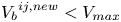 ${{V_{b}}}^{ij,{new}} < {V_{max}}$ where $i \in 1, 2$ and $j \in 3, 4, 5$).
E.3. Coarse graining of the liquid distribution
We denote by  ${{V_{b}}}^{ij}$ the volume of the liquid bridge between particles $i$ and $j$. The volume of the liquid film on particle $i$ is denoted by ${{V_{f}}}^{i}$ . We denote the Gaussian coarse-graining function with a width of one particle diameter by $\varPhi (x,z)_i$, centred around the position of particle $i$. We denote the normalised integral of the Gaussian coarse-graining function along the branch vector between particles $i$ and $j$ by $\psi (x,z)_{ij}$, see Weinhart et al. (Reference Weinhart, Thornton, Luding and Bokhove2012a). Then the liquid concentration at position $(x,z)$ is given by $Q = \sum _i {{V_{f}}}^{i} \varPhi (x,z)_i + \sum _{i,j} {{V_{b}}}^{ij} \psi (x,z)_{ij}$. See Weinhart et al. (Reference Weinhart, Thornton, Luding and Bokhove2012b) for more details and the notation.


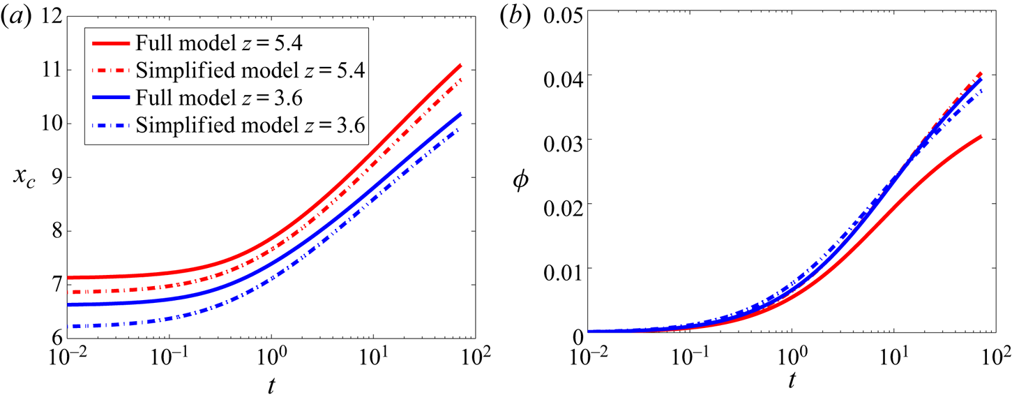


 Open access