


1. Introduction
The study of high-speed turbulent boundary layers is essential to determine the aerodynamic heating and drag on supersonic and hypersonic vehicles. The interest of the research community in this direction is fed by the technological advancements in the development of vehicles capable of sustained hypersonic flight in the atmosphere, sub-orbital flights and planetary re-entry (Urzay Reference Urzay2018). A crucial feature of these flows is their huge kinetic energy content compared with the thermal energy of the free-stream gas, which severely affects the near-wall turbulence structures. In fact, when such energetic flows are brought to rest by the presence of a wall, high thermal fluxes and intense pressure waves are generated, posing numerous technical challenges for the choice of surface materials. In the last decades, several theoretical relations have been proposed to grasp the relevant physical phenomena and understand the driving factors that are responsible for the deviations from classical laws developed for incompressible flows, on which several useful engineering models are based. However, the lack of reference data has always posed a major setback in the development of theoretical laws, in which key assumptions need to be validated.
The theory of supersonic flows relies on the so-called ‘compressibility transformations’, that were first presented in a broad and robust framework for both mean and fluctuating fields by Morkovin (Reference Morkovin1962). The key concept is that, when density fluctuations are small compared with the mean value, the mean velocity and Reynolds stress profiles in a compressible boundary layer can be mapped to equivalent incompressible distributions (Bradshaw Reference Bradshaw1977) by taking into account the mean density variation across the boundary layer. This assumption is the cornerstone at the base of the ‘Morkovin's hypothesis’, from which several consequences can be derived, as the Van Driest velocity scaling (Van Driest Reference Van Driest1956), consisting in a transformation of compressible flow profiles that takes into account the density variations to collapse them onto the incompressible laws. The Van Driest transformation has been extended to account for a finite wall heat flux by Trettel & Larsson (Reference Trettel and Larsson2016), who proposed an alternative formulation based on the log-layer scaling and near-wall momentum conservation. Although this transformation yields accurate results for internal flows like turbulent channels and pipes (Modesti & Pirozzoli Reference Modesti and Pirozzoli2016), some open questions remain for its application to non-adiabatic turbulent boundary layers (Volpiani, Bernardini & Larsson Reference Volpiani, Bernardini and Larsson2020a). Volpiani et al. (Reference Volpiani, Iyer, Pirozzoli and Larsson2020b) addressed this point proposing a mixed physical and data-driven transformation that shows an improved collapse with respect to the existing ones on turbulent boundary layers. Despite impressive results, the performance evaluation at higher Reynolds numbers and on different configurations (e.g. turbulent channels) is still undergoing. More recently, a total-stress-based transformation has been developed by Griffin, Fu & Moin (Reference Griffin, Fu and Moin2021), yielding very promising results through the entire inner layer regardless of the wall thermal condition. As before, more reference data at high Reynolds number are needed for the assessment of the performances of the proposed velocity scaling on collapsing on the incompressible profiles.
A key aspect of the theoretical study of compressible flows is the relation between velocity and temperature fields. Despite being nonlinearly coupled, a quantitative relationship between these fields was found firstly by Reynolds (Reference Reynolds1874), by means of similarity arguments between momentum and energy transport in wall-bounded flows that lead to a temperature-velocity relation. This concept is generally referred to as the ‘Reynolds analogy’, and was extended to laminar compressible boundary layers independently by Crocco (Reference Crocco1932) and Busemann (Reference Busemann1931) in adiabatic conditions. Later, a temperature-velocity relation was developed by Walz (Reference Walz1969) to account for the deviation of the Prandtl number from unity. This relation was improved empirically by Duan, Beekman & Martín (Reference Duan, Beekman and Martín2010), Duan & Martin (Reference Duan and Martin2011) and, more recently, by Zhang et al. (Reference Zhang, Bi, Hussain and She2014), who proposed a generalization to incorporate the effects of wall heat flux, that acquire relevance as the Mach number increases. The extension of these relations to fluctuating fields, initially proposed by Morkovin (Reference Morkovin1962), goes under the name of the strong Reynolds analogy (SRA), and consists in a set of relations between the velocity and temperature fluctuations. Although the SRA relations have been extensively used to formulate turbulence models, compressibility effects can undermine their accuracy, especially when large heat fluxes are considered. Subsequent extensions of SRA accounting for non-adiabatic wall conditions have been presented by Gaviglio (Reference Gaviglio1987), Rubesin (Reference Rubesin1990) and Huang, Coleman & Bradshaw (Reference Huang, Coleman and Bradshaw1995), and are still under validation for different flow conditions (Mach, Reynolds numbers and different wall temperatures) as computational and experimental data become available.
The advancement in the understanding of the physics involved in hypersonic turbulent boundary layers has been supported by DNS studies and experiments performed in the last two decades, although the current database is still very small compared with the subsonic and supersonic counterparts and almost exclusively limited to low Reynolds numbers. Experimental studies of high-speed flows have been historically conducted using hot-wire anemometry, that measures a combination of fluctuating mass flux and total temperature (see, for example, Smits, Hayakawa & Muck Reference Smits, Hayakawa and Muck1983). This technique is usually limited to the description of large-scale motions given the difficulties in resolving the near-wall flow scales and frequency response. More recently, particle image velocimetry has been employed in hypersonic turbulent boundary layers at Mach 4.9 and 7.5 by Tichenor, Humble & Bowersox (Reference Tichenor, Humble and Bowersox2013) and Williams et al. (Reference Williams, Sahoo, Baumgartner and Smits2018). Although this method allows direct measurements of spatially varying velocity fields, accurate measurements are not yet available especially on the wall-normal component of velocity or Reynolds stresses (Williams et al. Reference Williams, Sahoo, Baumgartner and Smits2018). Numerical simulations provide an alternative and effective method to investigate different aspects of these type of flows overcoming some technical difficulties of experiments, but are still limited by computational resources. One of the first studies of a hypersonic turbulent boundary layer up to Mach 6 has been conducted by Martin (Reference Martin2007), who focused on the initialization procedure to control flow conditions and reduce simulation transients. This was the first of a four part study continued by Duan et al. (Reference Duan, Beekman and Martín2010), Duan, Beekman & Martín (Reference Duan, Beekman and Martín2011) and Duan & Martin (Reference Duan and Martin2011), that extended the analysis on different features that are peculiar to highly compressible flows, namely the effect on the flow of Mach number (from 0.3 to 12), wall temperature condition ( $T_w/T_r$ ranging from 1 to 5.4) and high enthalpies. The implications of each change on the flow conditions have been assessed by looking at flow statistics, turbulent kinetic energy budget, coherent structures and their influence on the validity of the standard and modified SRA relations. An extension of the analysis on the effect of Mach number (2.5 to 20) has been provided by Lagha et al. (Reference Lagha, Kim, Eldredge and Zhong2011), with the objective to address the variations on turbulence statistics and near-wall turbulence structures. Another relevant study at very high Mach numbers with strong wall cooling has been recently presented by Huang et al. (Reference Huang, Nicholson, Duan, Choudhari and Bowersox2020). The effect of wall temperature has also been investigated in two separate studies by Xu et al. (Reference Xu, Wang, Wan, Yu, Li and Chen2021a,Reference Xu, Wang, Wan, Yu, Li and Chenb), who employed the Helmholtz decomposition first to characterize the variations on velocity and thermal statistics of a turbulent boundary layer at Mach 8 and then to study the implications on the kinetic energy transfer for different Mach numbers and wall temperature ratios. Zhang, Duan & Choudhari (Reference Zhang, Duan and Choudhari2018) carried out an extensive study analysing boundary layers with nominal free-stream Mach number ranging from 2.5 to 14 with different wall temperature conditions, representative of the operational conditions of different hypersonic wind tunnels. A recent comprehensive study on the effect of spatial evolution and Reynolds number has been performed by Huang, Duan & Choudhari (Reference Huang, Duan and Choudhari2022), considering a wide range of Mach numbers (from 2 to 11) with different amounts of wall cooling. At present, there is a lack of experimental and numerical studies corresponding to hypersonic diabatic turbulent boundary layers at moderate/high Reynolds number, which would be helpful to enrich our knowledge of compressible wall-bounded turbulence and to understand how the flow organization is affected by the combined variation of Mach number, Reynolds number and wall cooling. In this study we thus present novel DNS data to investigate the behaviour and the structure of isothermal supersonic (Mach 2) and hypersonic (Mach 6) zero-pressure-gradient turbulent boundary layers at moderate/high friction Reynolds numbers up to $Re_{\tau }\approx 2000$. First, we present instantaneous visualizations of the velocity and temperature fields, discussing the main differences between the two Mach numbers and with respect to supersonic adiabatic turbulent boundary layers reported in the literature. Then we focus on the existence in the boundary layer of large regions of uniform streamwise momentum, known in the literature as uniform momentum zones (Meinhart & Adrian Reference Meinhart and Adrian1995). We discuss the influence of compressibility on the properties of such zones and, for the first time, we document the existence of similar regions for the temperature field. Then, first- and second-order statistics for the velocity and thermodynamic variables are presented and discussed to highlight the influence of the various parameters. The final part of the study is dedicated to the analysis of the length scales of typical outer layer eddies, which are identified using power spectral densities of both the velocity and temperature fluctuations in the spanwise direction.
2. Computational set-up and numerical database
The physical model is based on the three-dimensional compressible Navier–Stokes equations for a viscous, heat conducting gas
 \begin{equation} \left.\begin{array}{c} \displaystyle\dfrac{\partial \rho}{\partial t}+\dfrac{\partial (\rho u_j)}{\partial x_j}=0,\\ \displaystyle\dfrac{\partial (\rho u_i)}{\partial t}+\dfrac{\partial (\rho u_i u_j)}{\partial x_j}+\dfrac{\partial p}{\partial x_i}-\dfrac{\partial \sigma_{ij}}{\partial x_j}=0,\\ \displaystyle\dfrac{\partial (\rho E)}{\partial t}+\dfrac{\partial (\rho E u_j+pu_j)}{\partial x_j}-\dfrac{\partial (\sigma_{ij}u_i-q_j)}{\partial x_j}=0, \end{array}\right\} \end{equation}
where  $\rho$ is the density, $u_i$ denotes the velocity component in the ith Cartesian direction ( $i=1,2,3$), $p$ is the thermodynamic pressure, $E=c_v T+u_i u_i/2$ the total energy per unit mass and
 \begin{equation} \sigma_{ij}=\mu \left( \frac{\partial u_i}{\partial x_j}+\frac{\partial u_j}{\partial x_i}-\frac{2}{3}\frac{\partial u_k}{\partial x_k}\delta_{ij}\right), \quad q_j={-}k\frac{\partial T}{\partial x_j}, \end{equation}
represent the viscous stress tensor and the heat flux vector, respectively. The molecular viscosity  $\mu$ is assumed to follow the Sutherland's law
 \begin{equation} \frac{\mu}{\mu_{\infty}}=\left(\frac{T}{T_{\infty}}\right)^{1/2} \frac{1+C/T_{\infty}}{1+C/T}, \end{equation}
where  $C=110.4$ K, $T_{\infty }=100.0$ K and $\mu _{\infty }=6.929\times 10^{-6}$ kg/(m s). The thermal conductivity $k$ is related to the viscosity by the expression $k=c_p \mu /Pr$, where $c_p$ is the specific heat at constant pressure and the Prandtl number is $Pr=0.72$. Since the temperature field ranges between 100 to 540 K for the hypersonic case, minor deviations from constant specific heat assumption are expected (Anderson Reference Anderson2006). Therefore, we assume all cases to fall within the perfect gas regime. The investigation of high-entalphy effects that involve the implementation of a chemically reacting model can be found in other studies, e.g. Passiatore et al. (Reference Passiatore, Sciacovelli, Cinnella and Pascazio2021, Reference Passiatore, Sciacovelli, Cinnella and Pascazio2022) and Di Renzo & Urzay (Reference Di Renzo and Urzay2021). The equations are discretised on a Cartesian grid and solved using the in-house code STREAmS (Bernardini et al. Reference Bernardini, Modesti, Salvadore and Pirozzoli2021), a high-fidelity solver targeted to canonical wall-bounded turbulent flows, freely available at https://github.com/matteobernardini/STREAmS. The code has been widely employed in the past to investigate supersonic wall-bounded turbulence, considering several canonical configurations, that include zero-pressure-gradient boundary layers, shock-wave boundary layer interactions, channel and pipe flows (Pirozzoli & Bernardini Reference Pirozzoli and Bernardini2011a; Bernardini & Pirozzoli Reference Bernardini and Pirozzoli2011b). The most recent solver version has been ported to multi graphics processing units architectures through the CUDA Fortran paradigm. One of the key features of the code is the availability of consolidated, high-order, energy-preserving schemes, applied in shock-free flow regions, that allow an efficient, accurate and stable discretization of the convective terms of the Navier–Stokes equations, free of numerical dissipation. A high-order shock capturing method (WENO scheme) is instead locally applied in shocked flow regions, identified by means of the Ducros shock sensor (Ducros et al. Reference Ducros, Ferrand, Nicoud, Weber, Darracq, Gacherieu and Poinsot1999). In the current version, a locally conservative formulation is also used for the viscous terms (De Vanna et al. Reference De Vanna, Benato, Picano and Benini2021), expanded to Laplacian for ensuring finite molecular dissipation at all resolved wavelengths.
In this work we present results obtained from DNS of diabatic turbulent boundary layers spanning a relatively large range of Mach and Reynolds numbers. The flow conditions of the simulations conducted are reported in table 1, where relevant computational parameters are also reported. Two hypersonic cases at Mach 5.86 are considered: the first at low friction Reynolds number, matching the M6Tw076 case of Zhang et al. (Reference Zhang, Duan and Choudhari2018), the second increasing  $Re_{\tau }$ up to 2000. Two additional simulations at the same friction Reynolds numbers are also carried out in the supersonic regime ( $M_{\infty }=2$) to enable a more comprehensive understanding of the effect of flow compressibility. Differently from our previous studies (Pirozzoli & Bernardini Reference Pirozzoli and Bernardini2011b), focused on adiabatic wall conditions, we here consider the case of cold walls, setting the wall-to-recovery temperature ratio $T_w / T_r = 0.76$, being
 \begin{equation} T_r=T_{\infty}\left(1+r \frac{\gamma-1}{2}M_{\infty}^2\right), \end{equation}
where  $r = 0.89$ is the recovery factor. This value satisfies the typical choice of $r=Pr^{1/3}$, which is generally accepted for turbulent boundary layers, and is consistent with the set-up of Zhang et al. (Reference Zhang, Duan and Choudhari2018). Although the ratio $T_w / T_r$ is matched for different Mach cases, it is worth highlighting that this choice corresponds to different values of the Eckert number, $Ec=(\gamma -1)M_{\infty }^2 T_{\infty }/(T_r-T_w)$, that are reported in table 1. The recent study by Wenzel, Gibis & Kloker (Reference Wenzel, Gibis and Kloker2022) has highlighted the relevance of this parameter in quantifying the combined effects of both Mach number and wall temperature on the boundary layer.
Table 1. Summary of parameters for DNS study. Grid spacings are given in wall units according to the stations selected in table 2. The values of  $\Delta y^+_{min}$ and $\Delta y^+_{max}$ refer to the wall-normal spacing at the wall and at the boundary layer edge, respectively. Here $Ec=(\gamma -1)M_{\infty }^2 T_{\infty }/(T_r-T_w)$ is the Eckert number and $\delta _{max}/\delta _{in}$ is the ratio between the maximum and inflow boundary layer thickness.

Table 2. Boundary layer properties at the selected stations. Here  $Re_{\tau }=\bar {\rho }_w u_{\tau } \delta /\bar {\mu _w}$, $Re_{\theta }=\rho _{\infty }u_{\infty }\theta /\mu _{\infty }$, $Re_{\delta _2}=\rho _{\infty }u_{\infty }\theta /\bar {\mu }_{w}$, $Re_{\tau }^*=\sqrt {\rho _{\infty } \tau _w}\delta /\mu _{\infty }$, $H=\delta ^*/\theta$ ( $\delta ^*$ and $\theta$ are the boundary layer displacement and momentum thickness, respectively); $B_q=q_w/(\rho _wC_pu_{\tau }T_w)$ is the dimensionless wall heat transfer rate.

The boundary layer is simulated in a rectangular box with spanwise periodic boundary conditions, purely non-reflecting boundary conditions for the outflow and the top boundary, and unsteady characteristic boundary conditions at the bottom wall, where isothermal wall temperature is enforced. The fully developed turbulent state is reached by means of a recycling-rescaling procedure (Pirozzoli, Bernardini & Grasso Reference Pirozzoli, Bernardini and Grasso2010), and the recycling length is placed at a distance of  $80 \delta _{in}$ from the inlet, $\delta _{in}$ being the boundary layer thickness (based on the 99 % of the external velocity $u_{\infty }$) at the inflow station. This distance is long enough to achieve a complete decorrelation of the fluctuations between the recycling station and the inflow plane (Morgan et al. Reference Morgan, Larsson, Kawai and Lele2011). The overall size of the computational domain of low-Reynolds-number cases is $L_x=100 \delta _{in}$, $L_y=30 \delta _{in}$, $L_z=8 \delta _{in}$ while, for the high Reynolds, $L_x=120 \delta _{in}$, $L_y=30 \delta _{in}$, $L_z=9.2 \delta _{in}$. Table 1 summarizes the flow conditions and grid resolutions for each run, where $M_{\infty }$ is the free-stream Mach number and $Re_{\tau }$ is the friction Reynolds number, defined as the ratio between the boundary layer thickness ( $\delta$) and the viscous length scale $\delta _{\nu }=\bar {\nu }_w/u_{\tau }$, where $u_{\tau }=\sqrt {\tau _w/\bar {\rho }_w}$ is the friction velocity, $\tau _w$ is the mean wall shear stress and $\nu _w$ is the kinematic viscosity at the wall. Here $N_x$, $N_y$ and $N_z$ are the number of computational points employed for each spatial direction, $\Delta x^+$ and $\Delta z^+$ the uniform grid spacings in the streamwise and spanwise directions and $\Delta y^+$ represents the non-uniform wall-normal grid spacing (the minimum and maximum values are reported). For the wall-normal direction, a newly developed stretching function described in Pirozzoli & Orlandi (Reference Pirozzoli and Orlandi2021) is employed, which provides a more favourable scaling of the number of grid points with the Reynolds number and has the natural property of yielding precisely constant resolution in terms of the local Kolmogorov length scale $\eta$ in the outer part of the wall layer while maintaining a uniform near-wall spacing. Moreover, the effective mesh spacing $\varDelta = (\Delta x \times \Delta y \times \Delta z)^{1/3}$ is always smaller than $4 \eta$, indicating that all the scales of turbulent motion are adequately resolved in the present computations. Simulations were carried out for a total period of $200 \delta _{in}/u_{\infty }$, collecting statistics with a sampling frequency of $0.1 \delta _{in}/u_{\infty }$, with $u_{\infty }$ being the free-stream velocity.
In our discussion, we use the symbols  $u$,
$u$,  $v$ and $w$ to denote the streamwise, wall-normal and spanwise velocity components and the decomposition of any variable is conducted using either the standard Reynolds decomposition ( $f=\bar {f}+f'$) or the density-weighted (Favre) representation ( $f=\tilde {f}+f{''}$), where $\tilde {f}=\overline {\rho f}/\bar {\rho }$. Actually, the Favre decomposition is generally preferred since we are dealing with highly compressible flows, but the observed Mach and Reynolds number effects are also apparent using Reynolds averages displaying only minor deviations. Table 2 summarizes the boundary layer parameters at selected locations where the turbulence statics are gathered.
3. Flow organization
3.1. Instantaneous visualization
We start providing an overview of the flow organization for the four cases here investigated by showing instantaneous density contours in a longitudinal plane in figure 1. For reference purposes, vertical lines are reported to mark the locations selected for the statistical analysis, which correspond to Reynolds numbers listed in table 2. The contours reveal the typical organization already found in low-speed and supersonic turbulent boundary layers (Smith & Smits Reference Smith and Smits1995; Duan, Choudhari & Wu Reference Duan, Choudhari and Wu2014), dominated by large-scale bulges inclined at approximately 45 $^\circ$, separating irrotational fluid from the inner rotational motion. A greater number of fine-scale features can be observed in the high-Reynolds-number cases, superimposed to a large-scale arrangement consisting of an array of rather uniform low-density bulges separated from a higher density free stream by a sharp interface. This scenario is shared by flow cases at $M = 2$ and $M = 6$, suggesting a relatively minor effect of the Mach number. Figures 2 and 3 show contours of the instantaneous velocity and temperature fluctuations for the high Reynolds cases in wall-parallel slices taken at two different locations, representative of both the inner ( $y^+=15$) and outer region ( $y/\delta = 0.2$) at the selected stations. At this friction Reynolds number, a clear scale separation is found between the turbulent eddies of the near-wall region and the outer layer motions. In particular, consistently with previous findings for adiabatic supersonic boundary layers (Bernardini & Pirozzoli Reference Bernardini and Pirozzoli2011a), a distinctive feature of the flow cases here analysed is the presence of large-scale structures, characterized by streamwise length scales of order $10 \delta$, which are usually referred to in the literature as superstructures (Marusic et al. Reference Marusic, McKeon, Monkewitz, Nagib, Smits and Sreenivasan2010). The signature of these large-scale eddies is well apparent in the outer portion of the boundary layer for both the velocity and temperature fluctuations, with an evident correlation between low-/high-speed momentum regions and high/low temperature streaks. A footprint of the outer layer structures can be observed in the near-wall region, where the small-scale velocity and temperature streaks typical of the near-wall cycle of turbulence are superposed to the large-scale organization inherited by the overlying motions. However, differently from previous observations for adiabatic walls (Bernardini & Pirozzoli Reference Bernardini and Pirozzoli2011a), the similarity between thermal and velocity streaks in the near-wall region of the present cold flow cases is less evident, particularly at Mach 2, where the distribution of temperature fluctuations appears more isotropic than that of the velocity field. In particular, while velocity streaks are clearly visible, temperature streaks are difficult to be detected in the near-wall region at $M=2$. This observation suggests that, despite the fixed value of $T_w/T_r$ for all flow configurations, the present supersonic flow cases are actually characterized by a greater importance of wall cooling. We note that, according to the discussion reported in Wenzel et al. (Reference Wenzel, Gibis and Kloker2022), this behaviour is consistent with the smaller value of the Eckert number characterizing the flow cases at Mach 2. As it will be discussed in the following sections, the different organization of the near-wall temperature field between supersonic and hypersonic cases is reflected by a distinctive shape of the temperature fluctuations variance and spectra. For completeness, wall-parallel slices close to the edge of the boundary layer (
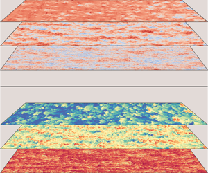
 $y/\delta = 0.9$ at the selected station) are also shown in figure 4. In this case, structural differences associated to the flow compressibility are not observed. Contours of both streamwise velocity and static temperature appear rather isotropic and reveal the existence of large, uniform regions of quiescent, cold free-stream fluid interspersed in the boundary layer. A clear association between high temperature turbulent regions of mushroom shape with low momentum zones is still visible at this height at both Mach numbers.

Figure 1. Contours of the instantaneous density field ( $\rho / \rho _{\infty }$) in a streamwise wall-normal plane for flow cases in table 1. The selected locations for this study are marked with vertical dashed lines in red. (a) Case M2L, (b) M6L, (c) M2H and (d) M6H.

Figure 2. Visualization of velocity and temperature fluctuations in a wall-parallel slice at  $y^+=15$. Velocity and temperature fluctuations are scaled with the mean velocity $\bar {u}$ and mean temperature $\bar {T}$, respectively. (a) Case M2H, velocity fluctuations, (b) M6H, velocity fluctuations, (c) M2H, temperature fluctuations and (d) M6H, temperature fluctuations.

Figure 3. Visualization of velocity and temperature fluctuations in a wall-parallel slice at  $y/\delta =0.2$. Velocity and temperature fluctuations are scaled with the mean velocity $\bar {u}$ and mean temperature $\bar {T}$, respectively. (a) Case M2H, velocity fluctuations, (b) M6H, velocity fluctuations, (c) M2H, temperature fluctuations and (d) M6H, temperature fluctuations.

Figure 4. Visualization of velocity and temperature fluctuations in a wall-parallel slice at  $y/\delta =0.9$. Velocity and temperature fluctuations are scaled with the mean velocity $\bar {u}$ and mean temperature $\bar {T}$, respectively. (a) Case M2H, velocity fluctuations, (b) M6H, velocity fluctuations, (c) M2H, temperature fluctuations and (d) M6H, temperature fluctuations.
3.2. Uniform momentum zones
Recent analyses have shown that instantaneous fields exhibit a peculiar property in a confined region of a turbulent boundary layer: uniform momentum zones. This property has been examined by several authors in the context of incompressible flows (Meinhart & Adrian Reference Meinhart and Adrian1995; Adrian, Meinhart & Tomkins Reference Adrian, Meinhart and Tomkins2000; De Silva, Hutchins & Marusic Reference De Silva, Hutchins and Marusic2016; Laskari et al. Reference Laskari, de Kat, Hearst and Ganapathisubramani2018), and only recently for hypersonic flows, although limited to low Reynolds numbers (Williams et al. Reference Williams, Sahoo, Baumgartner and Smits2018). A uniform zone of a given quantity is defined as a region in the  $x$–
$x$– $y$ plane with small variations along the wall-normal direction, implying the presence of local peaks in the histogram that collects all the sampled values of such quantity. The minima of these histograms, the least probable values, represent the local boundary between one zone and the other and are characterized by sharp gradients of the analysed quantity, in contrast to the generally uniform distribution between them (De Silva et al. Reference De Silva, Hutchins and Marusic2016). The presence of these zones have been attributed to hierarchical distribution of coherent structures within the boundary layer (De Silva et al. Reference De Silva, Hutchins and Marusic2016). The existence of these structures and their distribution along the boundary layer at different $Re_{\tau }$ is closely related to the fundamental hypothesis of the attached eddy model (Marusic & Monty Reference Marusic and Monty2019), which has been shown to reproduce flow statistics for wall-bounded turbulent flows (Perry & Marušić Reference Perry and Marušić1995) and to generate synthetic instantaneous velocity fields (De Silva et al. Reference De Silva, Hutchins and Marusic2016). Previous investigations focused on the analysis of the streamwise velocity, showing that uniform zones are present even at high Mach numbers (Williams et al. Reference Williams, Sahoo, Baumgartner and Smits2018). Here, mining our high Reynolds number database we confirm the presence of uniform zones of streamwise velocity and extend the analysis to the temperature field, for which a similar organization has never been documented. We also quantify the mean number of uniform zones $\bar {N}_{UZ}$ for both velocity and temperature fields in order to gauge the effect of the Mach number. This analysis is conducted at the highest Reynolds number in the present database, given the wider range of scales of turbulent motions which can be directly associated to the presence of uniform zones, particularly in the logarithmic region. Following the set-up of De Silva et al. (Reference De Silva, Hutchins and Marusic2016), the extracted instantaneous fields span roughly 2000 viscous units in the streamwise direction (which corresponds to a boundary layer length $\delta$) and extends through the whole boundary layer thickness in the wall-normal direction. To quantify the mean number of uniform zones for streamwise velocity and temperature, a total of 84 $xy$ planes were sampled well separated in the spanwise direction (more than $1\delta$) and in time (more than $2 \delta _{in}/u_{\infty }$). The selected quantity is then sampled at every point of the slice, except for the region outside the boundary layer. The latter condition requires a precise detection of the turbulent/non-turbulent interface (TNTI), that is not trivial, especially for compressible flows. Previous studies used a threshold in the kinetic energy defect (De Silva et al. Reference De Silva, Philip, Chauhan, Meneveau and Marusic2013) which produces inappropriate results in present highly compressible cases, since it does not consider the significant density fluctuations at the edge of the boundary layer. Therefore, we apply here a modified expression to detect the TNTI that involves the square of momentum defect in the streamwise and wall-normal direction, setting
 \begin{equation} M_{def}= \frac{(\rho U-\rho_{\infty}U_{\infty})^2+(\rho V-\rho_{\infty}V_{\infty})^2}{(\rho_{\infty}U_{\infty})^2}=0.001. \end{equation}
As for previous conditions, this expression vanishes when the flow becomes non-turbulent ( $\rho U \xrightarrow {} \rho _{\infty }U_{\infty }$ and $\rho V \xrightarrow {} \rho _{\infty }V_{\infty }=0$) and increases its value progressively towards the wall ( $M_{def}=1$). The fundamental difference is in the inclusion of the density inside the velocity defect, which better accounts for its contribution in the boundary layer edge. Its performances can be observed in figure 5 showing the iso-level $M_{def}=0.001$ (black line) on top of vorticity contours for both supersonic and hypersonic cases as a visual indicator of the turbulent region. A sensitivity study has been conducted on the threshold value showing minor deviations from the present contours for both flow cases. Further confirmation is given by figures 6 and 7 in which (3.1) correctly represents the boundary between the fluctuating field inside the boundary layer and the free stream for both $U$ and $T$. Figures 6 and 7 collect histograms and contours for cases M2H and M6H of the computed uniform zones for the velocity and temperature field. Similarly to the procedure of Laskari et al. (Reference Laskari, de Kat, Hearst and Ganapathisubramani2018), each histogram has been computed with a bin width of $0.5 u_{\tau }$ and the relative peak-finding algorithm considers a set of thresholds necessary to uniquely determine the number of uniform zones (UZ). In particular, considering the maximum height of the histogram, $h_{max}$, we employed a minimum height threshold for a peak detection of $0.025 h_{max}$ and a limit on promincences of $0.1 h_{max}$. Although the latter condition showed a non-negligible sensitivity on the predicted number of zones $N_{UZ}$ (as noted by Laskari et al. Reference Laskari, de Kat, Hearst and Ganapathisubramani2018), the trends, that are discussed below, are stable since the threshold values do not affect the relative variation of the detected average uniform zones number. We therefore chose a parameter set that matches the average number of zones of De Silva et al. (Reference De Silva, Hutchins and Marusic2016) for the case M2H on streamwise velocity, and we discuss the relative changes with the Mach number. In each histogram the local maxima values, which indicate the presence of a uniform zone in each $xy$ slice of the represented quantity, have been highlighted. The peak-finding algorithm also automatically outputs the minima associated to the selected peaks, which are used to draw the iso-lines that separate one uniform zone from another. Figures 6 and 7 clearly reveal the existence of uniform zones for both $U$ and $T$, thus suggesting that, even in the hypersonic regime, the hypothesized turbulent structures responsible for such zonal arrangement in low-speed flows (Adrian et al. Reference Adrian, Meinhart and Tomkins2000) are important in determining the flow organization of both the streamwise momentum and static temperature. After averaging multiple flow samples, we find a mean number of uniform zones for velocity of 3.6 for case M2H and 2.5 for case M6H. For the temperature, these values become 5.9 for case M2H and 4.9 for case M6H. From the computed values, we observe that the mean number of temperature zones is always greater than what was found for the velocity (there is a factor of roughly 1.6 for the case M2H and 2 for the case M6H), and that the hypersonic case exhibits a lower average number of zones for both quantities. We attribute these effects to the combined influence of the non-unit Prandtl number and diabatic wall, which decreases the degree of (anti)-correlation between velocity and temperature fluctuations. The zonal arrangement found for the temperature field supports the considerations of Pirozzoli & Bernardini (Reference Pirozzoli and Bernardini2011b), who concluded that this quantity can be considered an attached variable, similarly to the behaviour of streamwise velocity. However, higher-Reynolds-number cases spanning more than one order of magnitude are needed to confirm that the average number of zones follows a logarithmic distribution. It is also worth pointing out that we do not find a clear indication of uniform zones for the total temperature, being its fluctuations homogeneously distributed especially in the outer part of the boundary layer (not shown).

Figure 5. Contours of vorticity for case M2H (a) and M6H (b) represented with colours in the range [0–10]. The black line represents the TNTI defined with condition (3.1).

Figure 6. Uniform momentum zones of  $U$ and $T$ in an instantaneous field for the case M2H. The left column shows the computed histograms of the quantity in the selected $xy$ plane, with the associated maxima that indicate the presence of a uniform zone (blue circles). The right column shows the contours highlighting the boundary between each uniform zone and the instantaneous TNTI. Results are shown for (b) $U/(U_{\infty })$ and (d) $T/T_{\infty }$.

Figure 7. Uniform momentum zones of  $U$ and $T$ in an instantaneous field for the case M6H. The left column shows the computed histograms of the quantity in the selected $xy$ plane, with the associated maxima that indicate the presence of a uniform zone (blue circles). The right column shows the contours highlighting the boundary between each uniform zone and the instantaneous TNTI. Results are shown for (b) $U/U_{\infty }$ and (d) $T/T_{\infty }$.
4. Mean flow statistics
In this section several compressibility transformations and temperature-velocity relations are tested using the present DNS database. The scope of the former is to account for compressibility effects in wall-bounded flow statistics in order to recover the incompressible behaviour. The latter theoretical laws aim at predicting the relation between the mean temperature and velocity profile in compressible flows. Concerning the mean velocity, we first consider the classical velocity scaling proposed by Van Driest (Reference Van Driest1951) and that recently introduced by Trettel & Larsson (Reference Trettel and Larsson2016). While the former represents a density-weighted rescaling of the mean velocity profile, the latter is grounded on the log-layer scaling and near-wall momentum conservation to provide a transformation which is primarily tuned on turbulent channel flows with cooled walls. We further consider the recent scaling laws proposed by Volpiani et al. (Reference Volpiani, Iyer, Pirozzoli and Larsson2020b) and Griffin et al. (Reference Griffin, Fu and Moin2021), where the former takes advantage of a data-driven approach, while the latter is based on the total stress equation using different sets of hypotheses for the viscous and turbulent stress parts. According to Modesti & Pirozzoli (Reference Modesti and Pirozzoli2016), all the above transformations (except Griffin et al. Reference Griffin, Fu and Moin2021) can be expressed in terms of mapping functions  $f_{I}$ and $g_{I}$ for wall distance $y_{I}$ and mean velocity $u_{I}$, denoting the equivalent incompressible distributions obtained from the transformation $I$,
$I$,
 \begin{equation} y_{I}=\int_0^yf_I\, {\rm d} y ,\quad u_I=\int_0^{\tilde{u}} g_I \,{\rm d}\tilde{u}. \end{equation}
Using this convenient formulation, the aforementioned transformations are presented in table 3, where  $R=\bar {\rho }/\bar {\rho }_w$ and $M=\bar {\mu }/\bar {\mu }_w$. As mentioned above, the transformation of Griffin et al. (Reference Griffin, Fu and Moin2021) is based on the total stress equation, written in terms of a generalized non-dimensional mean shear $S_t^{+}=\partial U_t^+ / \partial y^*$, where the subscript $t$ means total and the superscripts $+$ and $*$ indicate inner and semilocal scaled variables, respectively. The latter are defined as $y^*=y/\delta _{\nu }^*$, where $\delta _{\nu }^*=\bar {\mu }/(\bar {\rho }u_{\tau }^*)$ and $u_{\tau }^*=\sqrt {\tau _w/\bar {\rho }}$. The equation reads as
 \begin{equation} \tau^+ = S_t^+ \left( \frac{\tau_v^+}{S_{TL}^+}+ \frac{\tau_R^+}{S_{eq}^+}\right), \end{equation}
where  $\tau _v^+$ and $\tau _R^+$ are the scaled viscous and Reynolds shear stresses (whose sum is equal to $\tau ^+$), while $S_{TL}^+=\partial U_{TL}^+ / \partial y^*$ and $S_{eq}^+=\partial U_{eq}^+ / \partial y^*$ are the generalized non-dimensional mean shear stresses derived for the viscous region (the subscript ‘ $TL$’ indicates accordance with the Trettel and Larsson velocity transformation) and for the log layer (the subscript ‘ $eq$’ indicates the assumption of turbulence quasi-equilibrium).
Table 3. Compressibility transformations for wall distance and mean velocity according to (4.1), where  $R=\bar {\rho }/\bar {\rho }_w$ and $M=\bar {\mu }/\bar {\mu }_w$.

Figure 8 shows the transformed mean velocity profiles  $u^+_{VD}$, $u^+_{TL}$, $u^+_{VI}$ and $u^+_{GR}$ for each case in order to assess the ability in collapsing compressible mean velocity profiles on the incompressible law-of-the-wall. The mean velocity profiles scaled using the various transformations well conform with the linear behaviour of the viscous sublayer ( $y^+<5$) for the chosen wall temperature conditions. Previous studies (Duan et al. Reference Duan, Beekman and Martín2010) observed a decrease of the Van Driest transformed mean slope with the increase of the cooling rate, but higher values of wall heat transfer $B_q$ were considered. Concerning the buffer and log layer, both the Van Driest and Trettel and Larsson transformations are less accurate in collapsing the velocity profiles onto the log-law distribution, yielding to a mismatch of the additive constant that is particularly evident for hypersonic flow cases and the Trettel and Larsson formula. Similar findings have been reported at lower Reynolds numbers by Zhang et al. (Reference Zhang, Duan and Choudhari2018), who suggested this discrepancy might be due to the influence of the wake component on the log region, and by Griffin et al. (Reference Griffin, Fu and Moin2021), who showed that the Trettel and Larsson transformation should only be valid in the viscous layer. In this regard, the fundamental assumptions of the Van Driest transformation are strictly applicable to adiabatic walls, and even in this case some authors reported its inaccuracy in collapsing profiles in the wake region for different Mach numbers (e.g. Duan et al. Reference Duan, Beekman and Martín2011; Wenzel et al. Reference Wenzel, Selent, Kloker and Rist2018). However, we note that the case M2L appears to agree well with the adiabatic counterpart of Pirozzoli & Bernardini (Reference Pirozzoli and Bernardini2011b). Looking at the performance of the two most recent transformations, an excellent collapse through the whole boundary layer can be observed for both Volpiani and Griffin for all cases of the present database, which demonstrates the capability of both approaches in accounting for the compressibility effect in a relatively wide range of Mach and Reynolds numbers. The only difference is detected in the wake region, where the GR transformation appears more efficient at collapsing the two high Mach numbers, independently of $Re_{\tau }$ (see insets of figure 8). Since the accuracy of the two scaling laws is comparable, the present database cannot assess which of the two proposals gives better results for the present conditions. We also remark that the proposed transformation of Griffin et al. (Reference Griffin, Fu and Moin2021) excellently behaves even using the constant-stress-layer assumption ( $\tau ^+ \approx 1$), with deviations not exceeding the $0.3\,\%$ from the standard one.

Figure 8. Mean velocity profiles at stations listed in table 2 scaled according to various compressibility transformations. The results are compared with the linear law  $u^+= y^+$ and the log law $u^+= 1/0.41 \ln (y^+)+5.2$. Transformed velocity profiles according to Van Driest (Reference Van Driest1951) are compared with the supersonic adiabatic case of Pirozzoli & Bernardini (Reference Pirozzoli and Bernardini2011b) at $M=2$ and $Re_{\tau }=450$. (a) Van Driest, (b) Trettel and Larsson, (c) Volpiani et al. and (d) Griffin et al.
Figure 9 shows the profiles of mean total and static temperature as a function of  $y/\delta$. The latter is also plotted in wall units in the inset of the figure, to highlight the profile behaviour in the near-wall region ( $y^+<25$). The presence of a temperature peak can be observed close to the wall ( $y^+\approx 5$) due to aerodynamic heating, that is more prominent and closer to the wall at high Mach number. The flatter mean temperature profile in the near-wall region at $M=2$ that is caused by the combination of the lower Mach number and the wall diabatic condition is consistent with the weaker temperature fluctuations observed in the discussion of figure 4 and in the following § 5.3. The total temperature displays an overshoot in the outer portion of the boundary layer that is larger at Mach 6, and apparently independent of the Reynolds number. Panels (c) and (d) display the mean temperature as a function of the mean velocity for all flow cases here investigated. Since the pioneering work of Reynolds (Reference Reynolds1874), several studies attempted to find a theoretical relationship between mean temperature and velocity fields, adjusting the general quadratic dependence to account for deviations of Prandtl number from unity and finite heat fluxes. The classical relationship of Walz (Reference Walz1969) has shown to behave well in adiabatic turbulent boundary layers, while decreasing its performances as wall cooling increases (Duan et al. Reference Duan, Beekman and Martín2010). Duan & Martin (Reference Duan and Martin2011) tackled this problem by proposing an empirical relation accounting for finite wall flux, that was later generalized by the work of Zhang et al. (Reference Zhang, Bi, Hussain and She2014). Here, DNS results are compared with the classical relation of Walz (Reference Walz1969),
 \begin{equation} \frac{\bar{T}}{T_{\infty}}=\frac{T_w}{T_{\infty}}+\frac{T_r-T_w}{T_{\infty}}\frac{\bar{u}}{U_{\infty}}+ \frac{T_{\infty}-T_r}{T_{\infty}}\left(\frac{\bar{u}}{U_{\infty}}\right)^2, \end{equation}
and the modified relation of Zhang et al. (Reference Zhang, Bi, Hussain and She2014) which explicitly accounts for the finite wall heat flux
 \begin{equation} \frac{\bar{T}}{T_{\infty}}=\frac{T_w}{T_{\infty}}+\frac{T_{rg}-T_w}{T_{\infty}}\frac{\bar{u}}{U_{\infty}}+ \frac{T_{\infty}-T_{rg}}{T_{\infty}}\left(\frac{\bar{u}}{U_{\infty}}\right)^2, \end{equation}
where  $T_{rg}=T_{\infty }+r_g U_{\infty }^2/(2 c_p)$ and $r_g=2 c_p (T_w-T_{\infty })/U_{\infty }^2-2 \, Pr \, q_w/(U_{\infty } \tau _w)$. Figure 9 reveals that the modified version proposed by Zhang et al. (Reference Zhang, Bi, Hussain and She2014) yields more accurate results at both Reynolds numbers than the classical relation of Walz, being able to capture the effects of the wall heat flux that exists in the present case of a cooled wall. Although the mismatch showed by Walz's law is visible, it falls within $3\,\%$ of the DNS values (the maximum deviations being at high Reynolds numbers). The authors attribute this behaviour to the wall cooling that is not intense enough to stress the limitations of this law. This finding is in accordance with the study of Duan et al. (Reference Duan, Beekman and Martín2011), that reports deviations up to $10\,\%$ when testing more extreme diabatic cases, e.g. $T_w/T_r=0.18$. The effect of the Reynolds number on the profiles is not significant, with the only visible difference being a slight decrease of the agreement with Walz's law at high Reynolds numbers.

Figure 9. Temperature profiles as a function of the wall-normal distance and mean velocity for all cases listed in table 2. Panels (a) and (b) show the profiles of the mean total temperature and mean temperature along the wall-normal distance  $y/\delta$. The inset shows the profiles in the near wall. Panels (c) and (d) show the mean temperature profile against mean velocity at low and high Reynolds numbers, compared with the classical law of Walz (Reference Walz1969) and the modified relation of Zhang et al. (Reference Zhang, Bi, Hussain and She2014).
5. Fluctuation statistics
5.1. Reynolds stresses
Reynolds stresses vs wall-normal distances are reported in figure 10 using the Morkovin transformation
 \begin{equation} (u_i^*)^2=\frac{\widetilde{u_i^{''2}}}{u_{\tau}^2}\frac{\bar{\rho}}{\bar{\rho}_w} , \quad (uv)^*=\frac{\widetilde{u{''}v{''}}}{u_{\tau}^2}\frac{\bar{\rho}}{\bar{\rho}_w}, \end{equation}
which should collapse compressible data to the incompressible ones (Morkovin Reference Morkovin1962). The profiles are shown as a function of the wall distance rescaled in wall units  $y^+$ and semilocal scaling $y^*$. For reference purposes, low-Reynolds-number cases are compared with the results of a low-speed turbulent boundary layer at $Re_{\tau }=445$ simulated by Jiménez et al. (Reference Jiménez, Hoyas, Simens and Mizuno2010), while the high-Reynolds-number cases are compared with the incompressible counterpart at $Re_{\tau }=1989$ computed by Sillero et al. (Reference Sillero, Jiménez and Moser2013). The figures reveal the relevant role played by both Mach and Reynolds numbers, leading to distinct and well-visible effects on the distribution of the various Reynolds stress components. Supersonic cases at both Reynolds numbers are in good agreement with their low-speed counterparts at matching $Re_{\tau }$, the most significant difference being an increase with the Mach number of the peak of the streamwise velocity fluctuations, already observed in previous investigations (Duan et al. Reference Duan, Beekman and Martín2011). The influence of wall cooling in this regard is believed to be minor given the good accordance of case M2L with the adiabatic case of Pirozzoli & Bernardini (Reference Pirozzoli and Bernardini2011b). The wide Reynolds number range covered by the present database allows us to appreciate the distinctive effect of the outer layer motions, whose relevance is known to increase with the Reynolds number, that provide large-scale contributions to the fluctuation intensities of the wall-parallel velocity components even in the near-wall region. Such distant eddies, usually referred to as ‘inactive motions’, are expected to induce a logarithmic growth with $Re_{\tau }$ of both $u$ and $w$ in the low-speed regime (Marusic & Monty Reference Marusic and Monty2019), here confirmed in the supersonic regime. The Reynolds number effect on the wall-normal velocity component and Reynolds shear stress appears as a plateau that corresponds to the formation of an equilibrium layer, again without a significant influence of the Mach number in the supersonic regime. Furthermore, at high Reynolds and Mach numbers, we also note reduced fluctuation intensities of the wall-normal and spanwise velocity in the outer layer, suggesting a less efficient redistribution of the turbulent energy from the streamwise component to the other ones in hypersonic conditions. Concerning the accuracy of the Morkovin scaling of velocity fluctuations, it offers an accurate collapse of profiles at the same $Re_{\tau }$ but not at different Mach numbers when plotted against the $y^+$ coordinate. Although the semilocal scaling $y^*$ increases the discrepancies among different cases in the outer layer, it should be noted that the semilocal friction Reynolds number is not matched for present cases.

Figure 10. Inner-scaled turbulent velocity fluctuations and Reynolds shear stress scaled according to Morkovin as a function of the wall-normal distance  $y^+$ (a,c,e,g) and semilocal $y^*$ (b,d,f,h). Present results are compared with the incompressible DNS of Jiménez et al. (Reference Jiménez, Hoyas, Simens and Mizuno2010) at $Re_{\tau }=445$, Sillero, Jiménez & Moser (Reference Sillero, Jiménez and Moser2013) at $Re_{\tau }=1989$ and the supersonic adiabatic case of Pirozzoli & Bernardini (Reference Pirozzoli and Bernardini2011b) at $M=2$ and $Re_{\tau }=450$.
5.2. Turbulent kinetic energy budget
The balance equation of the turbulent kinetic energy  $k=1/2 \widetilde {u_i{''}u_i{''}}$ for a compressible boundary layer (according to the derivation of Zhang et al. Reference Zhang, Duan and Choudhari2018) is given by
 \begin{equation} \frac{(D\bar{\rho} k)}{Dt}=P+TT+\varPi-\phi+D+ST, \end{equation}
with
 \begin{gather} P={-}\bar{\rho} \widetilde{u_i{''}u_j{''}} \frac{\partial \widetilde{u_i}}{\partial x_j}, \end{gather}
 \begin{gather}TT={-}\frac{\partial }{\partial x_j}\left[\frac{1}{2} \bar{\rho} \,\widetilde{u_i{''}u_i{''}u_j{''}} \right], \end{gather}
 \begin{gather}\varPi={-}\frac{\partial }{\partial x_i}(\overline{p'u_i{''}})+\overline{p'\frac{\partial u_i{''}}{\partial x_i}}, \end{gather}
 \begin{gather}\phi=\overline{\sigma_{ij}'\frac{\partial u_i{''}}{\partial x_j}}, \end{gather}
 \begin{gather}D=\frac{\partial }{\partial x_j}(\overline{\sigma_{ij}'u_i{''}}), \end{gather}
 \begin{gather}ST={-}\bar{\rho}\tilde{k}\frac{\partial \tilde{u}_k}{\partial x_k}+\overline{u_i{''}}\left( \frac{\partial \bar{\sigma}_{ij}}{\partial x_j}-\frac{\partial \bar{p}}{\partial x_i}\right), \end{gather}
where  $P$ is the production term, $TT$ represents the turbulent transport, $\varPi$ includes the pressure diffusion and dilatation, $-\phi$ is the viscous dissipation, $D$ is the viscous diffusion and $ST$ includes all additional terms that arise when density is not constant. In figure 11 the budget terms have been normalized by the conventional inner and semilocal scalings. As noted by Zhang et al. (Reference Zhang, Duan and Choudhari2018) and Duan & Martin (Reference Duan and Martin2011), the semilocal scaling of Huang et al. (Reference Huang, Coleman and Bradshaw1995) has a better capability to collapse different profiles for different Reynolds and Mach numbers, although some discrepancies due to the effect of the latter are still present. In particular, while viscous dissipation appears almost independent of $Re$ and $Ma$ numbers in semilocal scaling, production and turbulent transport still show a Mach dependence. We highlight that dissipation and the sum of turbulent transport with production appear independent of Mach number for $y^+>20$, as highlighted by the inset of figure 11(b). The better scaling of the production term in the semilocal scaling is exploited to evaluate the turbulent production in the log-layer region using a pre-multiplied representation as a function of $y^*$, where equal areas represent equal contribution to the total production (figure 12a). As noted by Smits, McKeon & Marusic (Reference Smits, McKeon and Marusic2011) and Marusic et al. (Reference Marusic, McKeon, Monkewitz, Nagib, Smits and Sreenivasan2010), the contribution of the bulk production extends to the log layer as the Reynolds number increases, becoming a significant source term of turbulent energy even outside the buffer layer. It should be noted that the highest peak is exhibited by the case at the highest Reynolds and Mach numbers considered. We attribute this feature to an indirect Mach number effect on the friction Reynolds number in semilocal quantities, $Re_{\tau }^*$, that, for present cases, is higher at $M=6$ with respect to the corresponding $M=2$ cases. Another important feature is the ratio between turbulent production and dissipation shown in figure 12(b), which should be close to one in the log layer (Zhang et al. Reference Zhang, Bi, Hussain, Li and She2012). This feature is well attained in the first part of the log layer for all present cases when the semilocal scaling is used, collapsing all the profiles in this region around one. However, data also show an excess of turbulent production farther from the wall (but still in the log layer) for hypersonic profiles, which is balanced by an increased turbulent transport. We attribute this effect to a more intense interaction between the outer and inner region, stimulated by the relatively denser, colder and less viscous outer layer eddies, characterized by a higher momentum. Such large-scale eddies are thus able to exert a greater influence onto the inner region, which is consistent with the less efficient kinetic energy redistribution described in § 5.1, and with the discussion in Pirozzoli et al. (Reference Pirozzoli, Romero, Fatica, Verzicco and Orlandi2021), which argued that the excess of turbulent production in the log layer feeds inactive motions that do not contribute to the turbulent shear stress, but transfer energy to other locations of the flow.

Figure 11. Turbulent kinetic energy budget in (a) inner scaling and (b) semilocal scaling.

Figure 12. Turbulent kinetic energy production in pre-multiplied form (a) and the ratio between production and dissipation (b) as a function of  $y^*$.
5.3. Thermodynamic quantities
To gain insights on the fluctuations of thermodynamic variables, the root-mean-square (r.m.s.) profiles of density, temperature and pressure are shown in figure 13 in both inner wall and semilocal scaling. In the left column the inner wall scaling is shown (together with an adiabatic case of Pirozzoli & Bernardini (Reference Pirozzoli and Bernardini2011b) that matches the Mach and Reynolds numbers of our case M2L). We note that at high Mach number a peak of the density fluctuation intensity establishes near the edge of the boundary layer. This peak is a consequence of the higher mean density (lower temperature) that occurs far from the wall with respect to the wall mean value  $\rho _w$, especially at high Mach number. Actually, considering the corresponding semilocal scaling, where $\rho _{rms}$ is normalized also with the local value of the mean density $\bar {\rho }$ (panel b), we observe that the peak is smeared and the profile in the log layer is almost flat, so the increase of the local density fluctuations is controlled by the mean local density. Similar arguments, but with the opposite behaviour, hold for the temperature fluctuations (panels c and d). Comparing the inner and semilocal scaling for density and temperature intensities, it emerges that, although the qualitative behaviour of the profiles is generally more similar in semilocal scaling, there is a clear Mach number dependency. The relative fluctuation intensities of density and temperature increase with the Mach number, while both supersonic and hypersonic cases exhibit less intense temperature fluctuations with respect to the adiabatic profile. This behaviour is consistent with the qualitative discussion of figure 4 and with the flatter mean temperature profile exhibited at $M=2$; see figure 9. Actually, the coupling between the wall-normal velocity fluctuations and a more uniform mean temperature is less effective to produce temperature fluctuations (e.g. near-wall streaks). It should be remarked that the cold wall enhances this behaviour because it produces a near-wall local maximum of the mean temperature profile, explaining the important difference of present diabatic $M=2$ data with respect to the adiabatic case of Pirozzoli & Bernardini (Reference Pirozzoli and Bernardini2011b).

Figure 13. Profiles of r.m.s. thermodynamic properties in inner and semilocal scalings. Grey vertical lines indicate the boundary layer edge at low Reynolds numbers (dashed line) and high Reynolds numbers (dot-dashed line), respectively. Here  $M_{\tau }=u_{\tau }/\sqrt {\gamma R T_w}$ and $M_{\tau }^*=u_{\tau }^*/\sqrt {\gamma R\tilde {T}}$ are the friction Mach numbers in inner and semilocal scalings, respectively. Inner-scaled profiles are compared with the supersonic adiabatic case of Pirozzoli & Bernardini (Reference Pirozzoli and Bernardini2011b) at $M=2$ and $Re_{\tau }=450$. Results are shown for (a) $\rho _{rms}/(\gamma \rho _w M_{\tau }^2)$, (b) $\rho _{rms}/(\gamma \bar {\rho } M_{\tau }^2)$, (c) $T_{rms}/(\gamma T_w M_{\tau }^2)$, (d) $T_{rms}/(\gamma \tilde {T} M_{\tau }^2)$, (e) $p_{rms}/ \tau _w$ and (f) $p_{rms}/ \tau _w$.
Conversely, the pressure fluctuations exhibit a completely different dynamics. A good collapse of the profiles emerges only using the wall scaling when cases at fixed  $Re_\tau$ are considered, while the semilocal scaling is not able to provide better results. The pressure fluctuation intensity appears controlled by the Reynolds number and almost independent of Mach number, except the very near-wall region and the free stream, where the acoustic radiation increases with $M_{\infty }$.
Summarizing, it emerges that, while the density and temperature fluctuations are strongly influenced by the Mach number as expected, the pressure fluctuations appear decoupled and turbulence controlled, since strongly depending only on the friction Reynolds number.
5.4. Length scales
We now address the spatial organization of the turbulent and thermal energy by looking at the pre-multiplied spectra of the streamwise velocity  $k_z E_{uu}(k_z)$ and temperature fluctuations $k_z E_{tt}(k_z)$ as a function of the spanwise wavelength $\lambda _z =2 {\rm \pi}/k_z$, where $k_z$ denotes the spanwise wavenumber and $E_{uu}$, $E_{tt}$ are the spectral densities computed in the spanwise direction of the velocity component $u$ and temperature $T$, respectively. The maps reported in figure 14 show the variation of the spectra with the wall-normal location, in both inner and outer scalings for the high-Reynolds-number cases at Mach 2 and 6. Concerning the velocity fluctuations, all cases highlight the existence of a primary energy peak in the buffer layer at $y^+ \approx 15$ with associated spanwise wavelengths of ${O}(100)$ wall units, which is an expected feature of the near-wall cycle of turbulence self-sustainment. Far from the wall, a secondary peak is observed in the outer layer for both the supersonic and hypersonic cases, corresponding to wavelengths of ${O}(\delta )$ which is the signature of the large-scale organization of the velocity field (superstructures) in the log layer, extending its influence into the near-wall region. The location of the secondary peak ( $y/\delta \approx 0.1$) is in accordance with the results of Bernardini & Pirozzoli (Reference Bernardini and Pirozzoli2011a) and Tomkins & Adrian (Reference Tomkins and Adrian2005). The spectral maps for the temperature fluctuations reveal the presence of remarkable differences between the two Mach numbers. In particular, a strong inner peak is only observed in the hypersonic case (whereas a much less intense plateau region is present at $M=2$), located in the buffer layer ( $y^+ \approx 20$) at wavelengths comparable with those of the velocity structures. Temperature streaks in the near-wall region are not highlighted by the spectra of the supersonic flow case, in agreement with the qualitative observations of § 3. This behaviour is mainly attributed to the effect of wall cooling, which is more effective in the present flow cases at Mach 2 as measured in terms of the Eckert number (Wenzel et al. Reference Wenzel, Gibis and Kloker2022). On the contrary, the outer peak in the temperature spectra is present for both Mach numbers in correspondence of wavelengths comparable with that of the velocity field, although it appears to be displaced upwards in the supersonic flow case. The evaluation of velocity and temperature spectra allows us to quantify the typical length scales in the outer turbulent wall layer. According to the classical theory (Prandtl Reference Prandtl1925) and to the predictions of the attached eddies model (Perry & Marušić Reference Perry and Marušić1995), the typical size of the energetic eddies is proportional to their distance from the wall ( $l_m = k y$). Under the assumption of a constant-stress layer it directly leads to the logarithmic behaviour of the mean velocity profile. On the basis of a simple eddy-viscosity ansatz, an improved scaling has been proposed by Pirozzoli (Reference Pirozzoli2012) and later adapted to compressible flows by Modesti & Pirozzoli (Reference Modesti and Pirozzoli2016),
 \begin{equation} l_{12}^{*}(y) \sim (u_{\tau} \delta)\left(\frac{\partial \tilde{u}_{VD}}{\partial y} \right)^{{-}1/2}, \end{equation}
which has been demonstrated to yield accurate results for compressible channel flows. Here we propose a further improvement of this scaling, by using the local mean shear computed on the velocity profile transformed according to Griffin et al. (Reference Griffin, Fu and Moin2021),
 \begin{equation} l_{12, GR}^{*}(y) \sim (u_{\tau} \delta)\left(\frac{\partial \tilde{u}_{GR}}{\partial y}\right)^{{-}1/2}. \end{equation}
Equations (5.9) and (5.10) are used for the normalization of the spanwise wavelength  $\lambda _z$ and the results compared with the conventional normalization based on the boundary layer thickness $\delta$. Regarding the latter choice, other suitable outer scales have been tested, such as the enthalpy thickness and the Rotta thickness, showing essentially the same behaviour. Figure 15 shows the pre-multiplied spectra of the streamwise velocity $k_z E_{uu}(k_z)$ for all flow cases and compares the capability of the aforementioned scalings for the spanwise wavelength $\lambda _z$ to collapse profiles at different wall-normal distances $y/\delta$. Figure 16 reports the pre-multiplied spectra of the temperature fluctuations $k_z E_{tt}(k_z)$ using the previously introduced scalings for the wavelength. To account for the variation of turbulence intensity across the wall layer, spectra are normalized by $\widetilde {u^{''2}}$ and $\widetilde {T^{''2}}$, respectively, yielding $\hat {E}_{uu}$ and $\hat {E}_{tt}$. Looking at panels (a,d,g,j) of figure 15, it can be seen that all cases show a distinct peak at $\lambda _z\approx \delta$, which suggests that the turbulent eddies have a characteristic spanwise length similar to the boundary layer thickness. Panels (b,e,h,k) show an improved collapse of the spectra at all off-wall locations thanks to the normalization of $\lambda _z$ with $l_{12}^{*}$ (5.9), supporting the validity of the theory developed by Pirozzoli (Reference Pirozzoli2012) and the arguments made by Modesti & Pirozzoli (Reference Modesti and Pirozzoli2016) for the extension to the compressible regime. Panels (c,f,i,l) show a slight improvement in collapsing the spectral curves, especially for the velocity and temperature fluctuations of the high Reynolds number at Mach 6, that is attributed to the more accurate theory of Griffin et al. (Reference Griffin, Fu and Moin2021) for highly compressible flows, as also shown in section § 4.

Figure 14. Pre-multiplied spanwise spectra of velocity  $E_{uu}$ and temperature $E_{tt}$ fluctuations for cases M2H (a,c) and M6H (b,d). The colour map is shown in log scale.

Figure 15. Pre-multiplied spanwise spectra of streamwise velocity fluctuations as a function of  $\lambda _z/\delta$ (a,d,g,j), $\lambda _z/l_{12}^{*}$ (b,e,h,k) and $\lambda _z/l_{12,GR}^{*}$ (c,f,i,l) for flow cases M2L (a–c), M6L (d–f), M2H (g–i), M6H (j–l). Different colours correspond to different wall-normal distances in the range $\eta =y/\delta =0.2- 0.8$.

Figure 16. Pre-multiplied spanwise spectra of temperature fluctuations as a function of  $\lambda _z/\delta$ (a,d,g,j), $\lambda _z/l_{12}^{*}$ (b,e,h,k) and $\lambda _z/l_{12,GR}^{*}$ (c,f,i,l) for flow cases M2L (a–c), M6L (d–f), M2H (g–i), M6H (j–l). Different colours correspond to different wall-normal distances in the range $\eta =y/\delta =0.2-0.8$.
6. Conclusions
This study presents an analysis of the relevant statistics of DNS of zero-pressure-gradient turbulent boundary layers at Mach numbers 2 and 5.86 with friction Reynolds numbers up to 2000. The wall is assumed to be isothermal and cold with respect to the free-stream recovery temperature, which is the most frequent condition for aerospace applications. In particular, to discern the various effects we compare four cases that are representative of supersonic and hypersonic regimes at low and moderately high friction Reynolds numbers. All cases share the same value of the wall-to-recovery-temperature ratio (equal to 0.76), but are characterized by different values of the Eckert number. A qualitative analysis of the turbulent flow organization is performed by means of instantaneous visualizations of streamwise velocity on  $x$–
$x$– $y$ and $x$–
$x$– $z$ slices. We note important deviations from usual observations in adiabatic walls, resulting in a less evident similarity between thermal and velocity fields. In particular, the near-wall streaks of the temperature fluctuations disappear in strongly non-adiabatic cases. The instantaneous fields have also been scrutinized in a more quantitative way to determine the existence of uniform zones (De Silva et al. Reference De Silva, Hutchins and Marusic2016) for the streamwise velocity and temperature, never addressed before. To detect the TNTI, a modified expression of the kinetic energy defect is introduced to take into account the strong density variations associated to the hypersonic regime. We find that uniform zones of both $U$ and $T$ do exist in both supersonic and hypersonic turbulent boundary layers and we compute their average number for the high-Reynolds-numbers cases of the present database. We find a clear increase of the average number of uniform temperature zones with respect to that of the streamwise velocity, while both numbers decrease in the hypersonic case. The analysis of mean velocity profiles reveals that an impressive collapse of compressible data into the incompressible counterpart is obtained with the recent transformations of Volpiani et al. (Reference Volpiani, Iyer, Pirozzoli and Larsson2020b) and Griffin et al. (Reference Griffin, Fu and Moin2021), thus extending the validation of these relations to moderate/high Reynolds numbers. An excellent agreement with the relation proposed by Zhang et al. (Reference Zhang, Bi, Hussain and She2014) is also found for the mean temperature profiles as a function of the streamwise velocity, improving the classical law of Walz (Reference Walz1969). By analysing the velocity fluctuations, we observe that at high Mach numbers there is a less efficient redistribution of turbulent energy from the streamwise component to the other ones, in accordance with Zhang et al. (Reference Zhang, Duan and Choudhari2018). Further evidence of this phenomenon is found by analysing the turbulent kinetic energy budget, where we note that the semilocal scaling provides a better collapse of the curves both for $M_{\infty }$ and $Re_{\tau }$, with the main exception of production and transport terms showing a dependence on Mach number, especially in the log layer. We attribute this discrepancy to an increase of interaction between the inner and outer region of the boundary layer caused by the larger density differences occurring in the hypersonic flow cases. Concerning the fluctuations of the thermodynamics variables, we find that while temperature and density r.m.s. show a clear increase with the Mach number, the pressure appears dominated by the friction Reynolds number with a weak dependence on $M_{\infty }$ even in the hypersonic regime. The comparison with a reference adiabatic case of Pirozzoli & Bernardini (Reference Pirozzoli and Bernardini2011b) indicates that wall cooling induces a decrease of the intensity of temperature fluctuations in terms of wall units. The length scale analysis has been performed calculating the pre-multiplied spectra of velocity and temperature fluctuations in the spanwise direction. Consistently with findings in the incompressible regime, we observe two peaks for the velocity field, in the buffer and in the outer layer, respectively. Similarly, two peaks are present in the pre-multiplied spectra of the temperature fluctuations for the hypersonic flow cases, still associated to distinct motions in the near-wall region and in the outer layer. We find that the buffer layer peak disappears in the most non-adiabatic case at $M_{\infty } = 2$, in agreement with the qualitative observations on the absence of temperature streaks close to the wall. Finally, we present a quite accurate scaling of the streamwise velocity and temperature spectra in the spanwise direction at different wall distances considering the characteristic length scale provided by (5.10). This scaling uses the local velocity gradient based on the recent theory of Griffin et al. (Reference Griffin, Fu and Moin2021) in the length scale definition introduced by Modesti & Pirozzoli (Reference Modesti and Pirozzoli2016).
Acknowledgements
We acknowledge that the results reported in this paper have been achieved using the PRACE Research Infrastructure resource MARCONI 100 based at CINECA, Casalecchio di Reno, Italy, under project PRACE n. 2020225442.
Declaration of interests
The authors report no conflict of interest.


 Open access