


1. Introduction
The emerging field of active soft matter physics has gained considerable attention in the biophysics and bioengineering communities recently (Lauga & Powers Reference Lauga and Powers2009; Elgeti, Winkler & Gompper Reference Elgeti, Winkler and Gompper2015; Bechinger et al. Reference Bechinger, Di Leonardo, Löwen, Reichhardt, Volpe and Volpe2016; Gompper et al. Reference Gompper2020). Over the past few years, there has been a mounting research interest in designing and developing self-propelling microswimmers as they are set forth as model systems for understanding the fundamentals of out-of-equilibrium phenomena in physiology and cellular biology. Synthetic man-made self-propelled active swimmers are capable of propelling themselves autonomously through a liquid by converting the energy extracted from their surrounding host environment into useful mechanical work. They are thought to hold great promise for future biomedical and clinical applications such as drug delivery, biopsy, precision nanosurgery, diagnostic histopathology, and transport of curative substances to tumour cells and inflammation sites (Gao & Wang Reference Gao and Wang2014). Suspensions of active components have been shown to lead to the emergence of a wealth of intriguing collective phenomena and fascinating spatiotemporal patterns. Prime examples include the motility-induced phase separation (Tailleur & Cates Reference Tailleur and Cates2008; Speck et al. Reference Speck, Bialké, Menzel and Löwen2014), propagating density waves and swarms (Grégoire & Chaté Reference Grégoire and Chaté2004; Menzel Reference Menzel2012), and the emergence of active meso-scale turbulence (Wensink et al. Reference Wensink, Dunkel, Heidenreich, Drescher, Goldstein, Löwen and Yeomans2012; Dunkel et al. Reference Dunkel, Heidenreich, Drescher, Wensink, Bär and Goldstein2013; Doostmohammadi et al. Reference Doostmohammadi, Ignés-Mullol, Yeomans and Sagués2018).
Phoretic self-propulsion is a well-established mechanism of choice in active matter research (Illien, Golestanian & Sen Reference Illien, Golestanian and Sen2017). Unlike most of the remotely actuated swimmers that rely fully on an external field to propel themselves through aqueous media (Dreyfus et al. Reference Dreyfus, Baudry, Roper, Fermigier, Stone and Bibette2005; Wang et al. Reference Wang, Li, Mair, Ahmed, Huang and Mallouk2014; Han, Shields IV & Velev Reference Han, Shields IV and Velev2018; Driscoll & Delmotte Reference Driscoll and Delmotte2019), self-phoretic swimmers stand apart since they can achieve intrinsic self-propulsion solely by exploiting local physico-chemical interactions with the surrounding fluid medium, while inherently fulfilling the force- and torque-free constraints required for swimming at the micron scale (Golestanian, Liverpool & Ajdari Reference Golestanian, Liverpool and Ajdari2005, Reference Golestanian, Liverpool and Ajdari2007). Phoretic active colloids can be set to motion through an effective slip velocity resulting from local concentration gradients induced via surface chemical reactions (Sharifi-Mood, Koplik & Maldarelli Reference Sharifi-Mood, Koplik and Maldarelli2013; Michelin & Lauga Reference Michelin and Lauga2014; Ibrahim, Golestanian & Liverpool Reference Ibrahim, Golestanian and Liverpool2017). Various theoretical works have been devoted to uncovering the effect of particle shape (Popescu et al. Reference Popescu, Dietrich, Tasinkevych and Ralston2010; Nourhani & Lammert Reference Nourhani and Lammert2016; Michelin & Lauga Reference Michelin and Lauga2017; Ibrahim, Golestanian & Liverpool Reference Ibrahim, Golestanian and Liverpool2018) and geometric confinement (Uspal et al. Reference Uspal, Popescu, Dietrich and Tasinkevych2016; Mozaffari et al. Reference Mozaffari, Sharifi-Mood, Koplik and Maldarelli2016; Choudhary et al. Reference Choudhary, Chaithanya, Michelin and Pushpavanam2021) on the behaviour and dynamics of self-phoretic particles. The collective behaviour of multiple phoretic particles has been studied in a number of different contexts (Golestanian Reference Golestanian2012; Gelimson et al. Reference Gelimson, Zhao, Lee, Kranz, Wong and Golestanian2016; Saha, Ramaswamy & Golestanian Reference Saha, Ramaswamy and Golestanian2019).
Breaking the spatial symmetry is a main prerequisite to achieve phoretic self-propulsion at the low Reynolds numbers (Golestanian et al. Reference Golestanian, Liverpool and Ajdari2005). From an experimental standpoint, the most commonly followed approach to fulfil this physical requirement consists of chemically patterning the surface of active colloidal particles (Howse et al. Reference Howse, Jones, Ryan, Gough, Vafabakhsh and Golestanian2007; Walther & Müller Reference Walther and Müller2013; Ebbens et al. Reference Ebbens, Gregory, Dunderdale, Howse, Ibrahim, Liverpool and Golestanian2014; Das et al. Reference Das, Garg, Campbell, Howse, Sen, Velegol, Golestanian and Ebbens2015; Simmchen et al. Reference Simmchen, Katuri, Uspal, Popescu, Tasinkevych and Sánchez2016; Ebbens & Gregory Reference Ebbens and Gregory2018; Zhou et al. Reference Zhou, Chen, Han and Wang2019; Campbell et al. Reference Campbell, Ebbens, Illien and Golestanian2019; Popescu Reference Popescu2020). An alternative route to accomplishing self-phoretic locomotion without the need for micro-patterning is based on exploiting geometrical asymmetries to induce chemical gradients (Michelin & Lauga Reference Michelin and Lauga2015). Indeed, isotropic self-phoretic particles can swim by means of phoretic and hydrodynamic interactions with other inert (non-motile) particles by forming dynamical clusters of anisotropic geometry (Soto & Golestanian Reference Soto and Golestanian2014; Varma, Montenegro-Johnson & Michelin Reference Varma, Montenegro-Johnson and Michelin2018; Agudo-Canalejo & Golestanian Reference Agudo-Canalejo and Golestanian2019; Nasouri & Golestanian Reference Nasouri and Golestanian2020). Meanwhile, Lisicki, Michelin & Lauga (Reference Lisicki, Michelin and Lauga2016) demonstrated that internal phoretic flows can be induced solely by geometric asymmetries of chemically homogeneous surfaces.
In the present contribution, we employ a far-field approach to examine the diffusiophoretic motion of an isotropic active colloidal particle of spherical shape positioned near a finite-sized disk resting on a planar interface separating two immiscible fluid media. Even though several previous studies have examined in great detail the case of diffusiophoresis near a no-slip wall or a fluid–fluid interface of infinite extent, to the best of our knowledge, none of these works has addressed the question of how finite-size effects could alter the swimming dynamics of active colloids near confining boundaries. In a large variety of biologically relevant applications, accounting for finite-sized effects is of crucial importance to achieve a reliable and accurate description of different transport mechanisms at the micron scale. The present contribution is a first step towards characterizing such finite-size effects, paving the way for future theoretical investigations.
Here, we consider the situation in which the system preserves its axial symmetry. Despite its apparent simplicity, we will show that the point-particle approximation employed throughout this work, which has been used widely in the context of particle motion under confinement (Spagnolie & Lauga Reference Spagnolie and Lauga2012), has again proven to capture the system behaviour in a surprisingly accurate way. More elaborate analytical models that describe the behaviour of a truly extended particle of finite size could be the subject of future works in this topic.
We formulate the phoretic problem as a classical mixed-boundary-value problem, which we subsequently transform into a system of dual integral equations on the inner and outer domain boundaries. We perform an explicit calculation of the hydrodynamic flow field by making use of the Lorentz reciprocal theorem in fluid mechanics (Masoud & Stone Reference Masoud and Stone2019) to yield an analytical expression of the induced phoretic velocity normal to the interface. Moreover, we compare favourably our analytical predictions with fully resolved numerical boundary integral solutions. More importantly, we find that the active particle can be repelled from or attracted to the interface depending on the particle–interface distance relative to the disk size, the ratios of fluid viscosities, and solubilities of species in the two media bounded by the interface, in addition to the sign of the phoretic mobility and chemical activity. Consequently, the self-phoretic swimming behaviour can be controlled by tuning the physical and geometrical properties of the system adequately.
2. Problem formulation
We examine the axisymmetric motion of a spherical active colloidal particle near a thin impermeable circular disk, resting on a flat fluid–fluid interface. The interface extends infinitely in the plane  $z = 0$. The active particle is coated with a catalyst that promotes a chemical reaction converting fuel molecules to products. We denote by the subscript
  $+$ the parameters and variables in the upper fluid domain above the interface, for which
  $z > 0$, and by the subscript
  $-$ the parameters and variables in the region occupied by the fluid underneath the interface, for which
  $z < 0$. Here, we consider a general situation in which the interface separates two immiscible fluids with different properties such as alkane/water interfaces. We assume that the fluids in both domains are Newtonian and incompressible, with uniform dynamic viscosities
  $\eta _\pm$. An infinitely-thin disk of radius
  $R$ is positioned within the plane
  $z=0$ separating the two immiscible fluids. In addition, we suppose that the disk is chemically inert and is rigidly anchored at the interface. Accordingly, the disk remains motionless. The active particle of radius
  $a$ is immersed fully in the upper fluid medium at position
  $h$ on the symmetry axis of the disk. We denote by
  $D_\pm$ the diffusion coefficients of the fuel molecules in each fluid compartment; see Figure 1 for a schematic illustration of the system under investigation. In the following, we employ a far-field approach to describe the induced hydrodynamic and concentration fields. We note that the effect of thermal noise as well as number fluctuations in the chemical field have been ignored throughout our calculations (Golestanian Reference Golestanian2009).
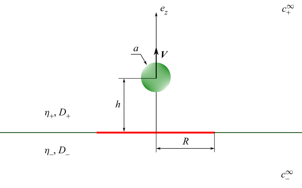
Figure 1. Schematic illustration of the system set-up. An active isotropic particle of radius  $a$ is located at position
  $h$ on the axis of an impermeable no-slip disk of radius
  $R$. The disk is embedded in an interface between two mutually immiscible fluids with dynamic viscosities
  $\eta _\pm$. We denote by
  $D_\pm$ the diffusion coefficient of the chemical, and by
  $c_\pm ^\infty$ the equilibrium far-field concentration of the solute in each fluid domain.
2.1. Equations for the concentration field
We suppose that the surface of the active particle emits or absorbs the solute with a uniform flux density  $Q$ such that
 \begin{equation} \left. -D_+\,\frac{\partial c_+}{\partial r} \right|_{r = a} = Q , \end{equation}
wherein  $Q$ can be positive or negative depending on whether the catalytic reaction is associated with a production (emission) or annihilation (absorption) of the solute.
At low Péclet numbers, the advection of the solute by the flow is negligible in relation to diffusion. Under these conditions, the evaluation of the solute distribution can be decoupled from that of the fluid flow. Accordingly, the stationary concentrations in the upper and lower domains are described by the Laplace equation
 \begin{equation} {\nabla}^2 c_\pm(\boldsymbol{r}) = 0 . \end{equation}
Equation (2.2) is subject to the boundary conditions of fixed concentration  $c_\pm ^\infty$ far away from the active particle as
  $| \boldsymbol {r} |\to \infty$. The surface of the finite-sized disk imposes a no-flux boundary condition
 \begin{equation} \left. \frac{\partial c_\pm}{\partial z} \right|_{z=0} = 0 \quad (\rho < R) . \end{equation}
Outside the disk, the fluid–fluid interface requires a continuous chemical flux,
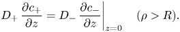 \begin{equation} \left. D_+\,\frac{\partial c_+}{\partial z} = D_- \, \frac{\partial c_-}{\partial z} \right|_{z=0} \quad (\rho > R) . \end{equation}
We define the dimensionless number
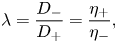 \begin{equation} \lambda = \frac{D_-}{D_+} = \frac{\eta_+}{\eta_-} , \end{equation}
assuming that the Stokes–Einstein relation is valid for diffusion in both domains.
In addition, we allow different solubilities of the chemical in the two liquid media (Domínguez et al. Reference Domínguez, Malgaretti, Popescu and Dietrich2016; Malgaretti & Harting Reference Malgaretti and Harting2021), leading to a discontinuity in concentration at the interface
 \begin{equation} \left. \ell c_+ = c_- \right|_{z = 0} \quad (\rho > R) , \end{equation}
where  $\ell$ is the partition constant. In an unperturbed fluid, it determines the ratio between equilibrium concentrations as
  $\ell = c_-^\infty / c_+^\infty$.
Equation (2.6) describes the discontinuity at the interface of the concentration field of the solute as a result of the difference in solubilities of species (Malgaretti, Popescu & Dietrich Reference Malgaretti, Popescu and Dietrich2018). Accordingly, we consider that the role of the interface is simply to permit a jump in the concentration field as a result of their distinct solvation energies.
2.2. Phoretic propulsion
We consider the frequently employed assumption of a short-range potential between the particle and solute molecules such that mutual interactions are limited to a thin boundary layer surrounding the active particle (Golestanian et al. Reference Golestanian, Liverpool and Ajdari2005, Reference Golestanian, Liverpool and Ajdari2007). Accordingly, the slip velocity at the surface of the active colloid,  $\mathcal {S}_{P}$, can be obtained from the tangential gradient of the concentration field as
 \begin{equation} \boldsymbol{v}_{S} = \left. \mu \boldsymbol{\nabla}_\parallel c_+ \right|_{\mathcal{S}_{P}} , \end{equation}
with  $\mu$ denoting the phoretic mobility that is defined from the profile of the local interaction potential between the particle and solute molecules. In addition,
 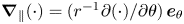 $\boldsymbol {\nabla }_\parallel (\cdot ) = (r^{-1} \partial (\cdot ) / \partial \theta ) \, \boldsymbol {e}_\theta$ stands for the tangential gradient along the surface of the sphere.
3. Solution for the concentration field
In the far-field limit, the active particle can be approximated conveniently as a point source. We express the solution of the Laplace equations for the concentration field in both fluid domains as a sum of a direct contribution  $C$ and the contributions of the boundary or the flux across the boundary
  $c_\pm ^*$:
 \begin{equation} c_+ = c_+^\infty + C + c_+^* , \quad c_- = c_-^\infty + c_-^* . \end{equation}
Here,  $C$ is the solution of (2.2) in an unbounded fluid medium subject to the constant flux boundary condition at the surface of the active particle stated by (2.1). Specifically,
 \begin{equation} C (\rho, z) = K \left( \rho^2 + \left(z-h\right)^2 \right)^{-{1}/{2}} , \end{equation}
where we have defined the length scale 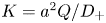 $K = a^2 Q/D_+$.
In addition,  $c_\pm ^*$ are the complementary (also often referred to as the image) solutions that are required to satisfy the boundary conditions prescribed at the fluid–fluid interface as well as at the surface of the finite-sized disk. Being harmonic functions, we express the image solutions in terms of Fourier–Bessel integrals of the form
 \begin{equation} c_\pm^* (\rho, z) = \int_0^\infty A_\pm (q)\,{\rm J}_0(q \rho)\,{\rm e}^{- q |z|} \, \mathrm{d} q , \end{equation}
with  ${\rm J}_0$ denoting the zeroth-order Bessel function of the first kind. Moreover, the wavenumber-dependent functions
  $A_\pm (q)$ will be determined subsequently from the underlying boundary conditions.
3.1. Formulation of the dual integral equations
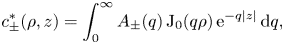
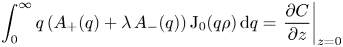
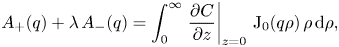
The equations for the inner problem ( $\rho < R$) can be obtained readily by inserting (3.1a,b) into (2.3), prescribing the no-flux boundary condition at the surface of the finite-sized disk, to obtain
 \begin{gather} \int_0^\infty q\,A_+(q)\,{\rm J}_0 (q \rho) \, \mathrm{d} q = \left. \frac{\partial C}{\partial z} \right|_{z=0} \quad (\rho < R) , \end{gather}
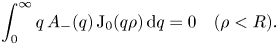 \begin{gather}\int_0^\infty q\,A_-(q)\,{\rm J}_0(q \rho) \, \mathrm{d} q = 0 \quad (\rho < R) . \end{gather}
 On the other hand, the equations for the outer problem ( $\rho >R$) follow from applying the boundary conditions imposed at the fluid–fluid interface given by (2.4) and (2.6):
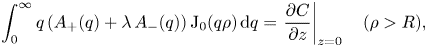 \begin{gather} \int_0^\infty q \left( A_+(q) + \lambda\,A_-(q) \right) {\rm J}_0 (q \rho) \, \mathrm{d} q = \left. \frac{\partial C}{\partial z} \right|_{z=0} \quad (\rho > R) , \end{gather}
 \begin{gather}\int_0^\infty \left( A_-(q) - \ell\,A_+(q) \right) {\rm J}_0(q \rho) \, \mathrm{d} q = \left. \ell C \right|_{z=0} \quad (\rho > R) . \end{gather}
 Equations (3.4) and (3.5) form a system of dual integral equations for  $A_\pm (q)$ on the inner and outer domain boundaries. Analytical solutions of such types of integral equations with Bessel function kernels can often be obtained by employing the theory of Mellin transforms (Titchmarsh Reference Titchmarsh1948; Tranter Reference Tranter1951). However, we choose to follow an alternative strategy using the well-established solution approach described by Sneddon (Reference Sneddon1960) and Copson (Reference Copson1961). In particular, we will show that the present system of dual integral equations can be reduced eventually to classical Abel integral equations, amenable to inversion in explicit form. We note that previously, this solution approach has been utilised frequently to solve diverse flow problems involving finite-sized boundaries. These include the determination of the viscous flow field induced by various types of singularities acting near an elastic disk possessing shear and bending deformation modes (Daddi-Moussa-Ider, Kaoui & Löwen Reference Daddi-Moussa-Ider, Kaoui and Löwen2019; Daddi-Moussa-Ider Reference Daddi-Moussa-Ider2020), near a no-slip disk (Kim Reference Kim1983; Daddi-Moussa-Ider et al. Reference Daddi-Moussa-Ider, Lisicki, Löwen and Menzel2020a, Reference Daddi-Moussa-Ider, Sprenger, Richter, Löwen and Menzel2021), or between two coaxially positioned rigid disks of the same size (Daddi-Moussa-Ider et al. Reference Daddi-Moussa-Ider, Sprenger, Amarouchene, Salez, Schönecker, Richter, Löwen and Menzel2020b; Daddi-Moussa-Ider Reference Daddi-Moussa-Ider2022). The present approach has also been employed to determine the electrostatic potential in a circular plate capacitor with disks of different radii (Paffuti et al. Reference Paffuti, Cataldo, Di Lieto and Maccarrone2016).
3.2. Solution of the dual integral equations
By combining the equations for the inner problem given by (3.4) and invoking (3.5a), it follows that
 \begin{equation} \int_0^\infty q \left( A_+(q) + \lambda\,A_-(q) \right) {\rm J}_0 (q \rho) \, \mathrm{d} q = \left. \frac{\partial C}{\partial z} \right|_{z=0} \end{equation}
applies for all values of  $\rho$. Accordingly, the Hankel transform can be applied on both sides of the equation to obtain
 \begin{equation} A_+(q) + \lambda\,A_-(q) = \int_0^\infty \left. \frac{\partial C}{\partial z} \right|_{z=0} \, {\rm J}_0(q \rho)\,\rho \, \mathrm{d} \rho , \end{equation}
which, upon inserting the expression for  $C(\rho, z)$ given by (3.2), leads us to
 \begin{equation} A_+(q) + \lambda\,A_-(q) = K {\rm e}^{{-}q h} . \end{equation}
To satisfy the equations for the outer domain, we choose a solution of the integral form
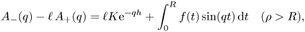 \begin{equation} A_-(q) - \ell\,A_+(q) = \ell K {\rm e}^{{-}q h} + \int_0^R f(t) \sin (q t) \, \mathrm{d} t \quad (\rho > R) , \end{equation}
where we have defined the integral functions
 \begin{equation} \mathcal{L}_m^n (\rho, t) = \int_0^\infty {\rm J}_n(q \rho) \sin \left( q t + m \, \frac{\rm \pi}{2} \right) \mathrm{d} q , \end{equation}
for  $m, n \in \{0,1\}$. It can be checked readily that (3.5b) is satisfied because
  $\mathcal {L}_0^0(\rho, t) = 0$ for
  $t< R<\rho$ (see (A 1) in Appendix A.) Solving (3.8) and (3.9) for
  $A_\pm (q)$ yields
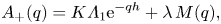 \begin{gather} A_+ (q) = K \varLambda_1 {\rm e}^{{-}q h} + \lambda\,M (q) , \end{gather}
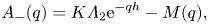 \begin{gather}A_- (q) = K \varLambda_2 {\rm e}^{{-}q h} - M (q) , \end{gather}
where we have defined  $\varLambda _1 = ( 1-\lambda \ell ) / ( 1+\lambda \ell )$ and
  $\varLambda _2 = 2 \ell / ( 1+\lambda \ell )$. Moreover,
 \begin{equation} M (q) ={-}\frac{1}{1+\lambda\ell } \int_0^R f(t) \sin (q t) \, \mathrm{d} t . \end{equation}
Substituting the expressions for  $A_\pm (q)$ given by (3.11) into either integral equation for the inner problem given by (3.4) yields
 \begin{equation} \int_0^\infty q\,M (q)\,{\rm J}_0 (q \rho) \, \mathrm{d} q = \frac{\varLambda_2 Kh}{\left( \rho^2 + h^2 \right)^{{3}/{2}}} \quad (\rho < R) . \end{equation}
To proceed further, we employ integration by parts to obtain
 \begin{equation} \int_0^R q\,f(t) \sin (q t) \, \mathrm{d} t = \varphi(q) +\int_0^R f'(t) \cos (q t) \, \mathrm{d} t , \end{equation}
wherein  $\varphi (q) = f(0) - f(R) \cos (q R)$. Correspondingly, (3.13) can be expressed
 \begin{equation} \int_0^R \mathcal{L}_1^0(\rho, t) f_2'(t) \, \mathrm{d} t = G(\rho) \quad (\rho < R) , \end{equation}
where we have interchanged the order of integration with respect to  $t$ and
  $q$, and defined for convenience
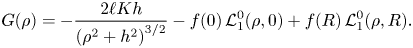 \begin{equation} G(\rho) ={-}\frac{2\ell K h}{\left( \rho^2 + h^2 \right)^{{3}/{2}}} - f(0)\,\mathcal{L}_1^0(\rho, 0) + f(R)\,\mathcal{L}_1^0(\rho, R) . \end{equation}
 It follows from (A 1) that  $\mathcal {L}_1^0(\rho, 0) = 1/\rho$ and
  $\mathcal {L}(\rho, R) = 0$ (because
  $\rho < R$ holds in the inner domain). Then (3.15) simplifies to
 \begin{equation} \int_0^\rho \frac{f'(t) \, \mathrm{d} t}{\left( \rho^2 - t^2 \right)^{{1}/{2}}} ={-}\frac{2\ell Kh}{\left( \rho^2 + h^2 \right)^{{3}/{2}}} - \frac{f(0)}{\rho} . \end{equation}
 Since  $f(0)$ is required to vanish for (3.17) to be defined at
  $\rho = 0$, the resulting equation for
  $f(t)$ reduces to a classical Abel integral equation. The latter represents a special form of the Volterra equation of the first kind possessing a weakly singular kernel (Carleman Reference Carleman1921; Smithies Reference Smithies1958; Anderssen, De Hoog & Lukas Reference Anderssen, De Hoog and Lukas1980). It admits a unique solution if and only if the radial function on the right-hand side is a continuously differentiable function (Carleman Reference Carleman1922; Tamarkin Reference Tamarkin1930; Whittaker & Watson Reference Whittaker and Watson1996). Its solution is obtained as
 \begin{equation} f(t) ={-}\frac{4}{\rm \pi}\,\frac{\ell K t}{t^2 + h^2} . \end{equation}
 By inserting the latter expression for  $f(t)$ into (3.12), we obtain
 \begin{equation} M (q) = \varLambda_2 K \int_0^R \frac{2}{\rm \pi}\,\frac{t \sin (q t)}{t^2+h^2} \, \mathrm{d} t . \end{equation}
 In particular, in the limit  $R \to \infty$ corresponding to an infinitely extended impermeable wall, we get
 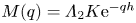 $M (q) = \varLambda _2 K {\rm e}^{-q h}$, leading to
  $A_+(q) = K {\rm e}^{-q h}$ and
  $A_-(q) = 0$.
Finally, by inserting the expression for  $M (q)$ into (3.11) and substituting the resulting expressions of
  $A_\pm (q)$ into (3.3), the solutions for the concentration field are obtained as
 \begin{gather} c_+^* (\rho, z) =\varLambda_1\,C(\rho, -z) + \lambda \, \tilde{c} (\rho, z) , \end{gather}
 \begin{gather}c_-^* (\rho, z) = \varLambda_2\,C(\rho, +z) - \tilde{c} (\rho, z) . \end{gather}
The first term in each expression is a simple image  $C(\rho,\pm z)$ that describes the effect of the fluid–fluid interface. The second term,
  $\tilde c(\rho,z)$, can be interpreted as the field induced by an effective source dipole distribution in the boundary that compensates the flux across the interface, such that the superposition of both terms obeys the zero-flux boundary condition. Here, the contribution resulting from the presence of the impermeable disk can be written in the form of a definite integral as
 \begin{equation} \tilde{c} (\rho, z) = \varLambda_2 K \int_0^R \frac{2}{\rm \pi}\,\frac{t \, \mathcal{U} (\rho, z, t)}{t^2 + h^2} \, \mathrm{d} t , \end{equation}
where we have defined
 \begin{equation} \mathcal{U} (\rho, z, t) = \int_0^\infty {\rm J}_0 (q \rho) \sin (q t)\,{\rm e}^{{-}q |z|} \, \mathrm{d} q . \end{equation}
 We will show below that an analytical evaluation of the latter improper integral is possible by invoking concepts from complex analysis. Using the substitution  $u = q \rho$, we obtain
 \begin{equation} \mathcal{U} (\rho, z, t) = \rho^{{-}1} \operatorname{Im} \left\{ \int_0^\infty {\rm J}_0 (u)\,{\rm e}^{{-}su} \, \mathrm{d} u \right\}, \end{equation}
with  $s = ( |z| - {\rm i}t )/\rho$. By recalling the Laplace transform of
  ${\rm J}_0 (u)$, which is given by
  $( 1+s^2 )^{-{1}/{2}}$, we obtain
 \begin{equation} \mathcal{U} (\rho, z, t) = \operatorname{Im} \left\{ \left( \rho^2 + \left( |z| - {\rm i}t \right)^2 \right)^{-{1}/{2}} \right\} . \end{equation}
Further, by evaluating the imaginary part, (3.24) can be expressed in the form
 \begin{equation} \mathcal{U} (\rho, z, t) = \left( \left( U-V \right)/2 \right)^{{1}/{2}} / U , \end{equation}
where we have defined
 \begin{equation} U = \left( ( \rho^2 + z^2 + t^2 )^2 - \left(2\rho t\right)^2 \right)^{{1}/{2}} , \quad V = \rho^2 + z^2 - t^2 . \end{equation}
 In the special case  $R\to \infty$, representing an infinitely extended impermeable wall, the image solution
 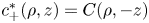 $c_+^*(\rho,z)=C(\rho,-z)$,
  $c_-^*(\rho,z)=0$ is recovered by noting that (see Appendix B for the proof)
 \begin{equation} \int_0^\infty \frac{t \, \mathcal{U} (\rho, z, t)}{t^2+h^2} \, \mathrm{d} t = \frac{\rm \pi}{2} \left( \rho^2 + \left( |z|+h \right)^2 \right)^{-{1}/{2}} . \end{equation}
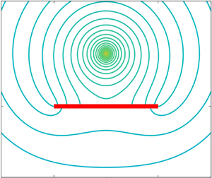
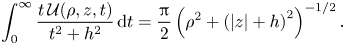
Exemplary contour plots illustrating the lines of equal concentration, also sometimes called isopleths, are shown in figure 2 for two different singularity positions above the interface while keeping the viscosity and solubility ratios equal to 1. The presence of the disk introduces an asymmetry in the form assumed by the lines of equal concentration owing to the no-flux boundary condition imposed at the surface of the disk. Analogous contour plots are shown in figure 3 upon varying the ratio of solubility between the two media.
Figure 2. Contour plots of the scaled concentration field around an active particle positioned at (a)  $h/R = 0.25$ and (b)
  $h/R = 1$ on the axis of a finite-sized impermeable disk of radius
  $R$ (shown in red) resting on a fluid–fluid interface with viscosity ratio
  $\lambda = 1$ and solubility ratio
  $\ell = 1$.
Figure 3. Contour plots of the scaled concentration field around an active particle positioned at  $h/R = 0.5$ for
  $\lambda = 1$ and solubility ratios (a)
  $\ell = 0.1$ and (b)
  $\ell = 10$.
4. Phoretic velocity
Al low Reynolds numbers, the dynamics of the viscous Newtonian fluids in the two fluid domains is governed by the steady Stokes equations (Kim & Karrila Reference Kim and Karrila2013)
 \begin{gather} \boldsymbol{\nabla} \boldsymbol{\cdot} \boldsymbol{v}_\pm = 0 , \end{gather}
 \begin{gather}-\boldsymbol{\nabla} p_\pm{+} \eta_\pm {\nabla}^2 \boldsymbol{v}_\pm = 0 , \end{gather}
where  $\boldsymbol {v}_\pm$ denotes the flow velocity, and
  $p_\pm$ denotes the pressure.
4.1. Lorentz reciprocal theorem
In lieu of solving directly the governing equations for fluid motion for the prescribed boundary conditions, we follow an alternative route based on the Lorentz reciprocal theorem (Stone & Samuel Reference Stone and Samuel1996; Happel & Brenner Reference Happel and Brenner2012). This approach has been used extensively in the context of phoretic swimming to determine the propulsion velocity of chemically active colloids suspended in an unbounded fluid medium (Popescu, Uspal & Dietrich Reference Popescu, Uspal and Dietrich2016; Oshanin, Popescu & Dietrich Reference Oshanin, Popescu and Dietrich2017), close to a planar no-slip wall (Crowdy Reference Crowdy2013; Uspal et al. Reference Uspal, Popescu, Dietrich and Tasinkevych2015; Yariv Reference Yariv2016), and near a chemically patterned surface (Uspal et al. Reference Uspal, Popescu, Tasinkevych and Dietrich2018; Popescu, Uspal & Dietrich Reference Popescu, Uspal and Dietrich2017), or to compute the stresslet field induced by active swimmers (Lauga & Michelin Reference Lauga and Michelin2016). Further, the reciprocal theorem has been adapted to describe the phoretic interaction of two active Janus particles (Sharifi-Mood, Mozaffari & Córdova-Figueroa Reference Sharifi-Mood, Mozaffari and Córdova-Figueroa2016; Nasouri & Golestanian Reference Nasouri and Golestanian2020), or to investigate the behaviour of a self-propelled active particle in a complex fluid (Lauga Reference Lauga2014; Elfring Reference Elfring2017).
According to the reciprocal theorem, two distinct solutions of the Stokes equations  $( \boldsymbol {v}, \boldsymbol {\sigma } )$ and
  $( \hat {\boldsymbol {v}}, \hat {\boldsymbol {\sigma }} )$ within the same fluid domain
  $\mathcal {D}$ bounded by a surface
  $\mathcal {S}$ are related to each other via
 \begin{equation} \int_\mathcal{S} \boldsymbol{n} \boldsymbol{\cdot} \boldsymbol{\sigma} \boldsymbol{\cdot} \hat{\boldsymbol{v}} \, \mathrm{d} S = \int_\mathcal{S} \boldsymbol{n} \boldsymbol{\cdot} \hat{\boldsymbol{\sigma}} \boldsymbol{\cdot} \boldsymbol{v} \, \mathrm{d} S , \end{equation}
with  $\boldsymbol {n}$ denoting the unit vector normal to the surface
  $\mathcal {S}$ pointing into the fluid domain. In the following, unhatted and hatted quantities will be used to refer to the flow properties in the main and model (also sometimes called auxiliary and dual) problems, respectively.
The reciprocal theorem can be extended easily to multiple fluid domains with continuity of velocity and stress at their interfaces. We will demonstrate in the following that the underlying boundary conditions imply a vanishing contribution to the surface integral over the fluid–fluid interface (Sellier & Pasol Reference Sellier and Pasol2011). By decomposing the fluid domain on both sides of the fluid–fluid interface, the reciprocal theorem in the upper domain is expressed as
 \begin{equation} \int_{\mathcal{S}_{P}} \left( \boldsymbol{v}_+ \boldsymbol{\cdot} \hat{\boldsymbol{\sigma}}_+{-} \hat{\boldsymbol{v}}_+ \boldsymbol{\cdot} \boldsymbol{\sigma}_+ \right) \boldsymbol{\cdot} \boldsymbol{n} \, \mathrm{d} S + \int_{\mathcal{S}_{I}} \left( \boldsymbol{v}_+ \boldsymbol{\cdot} \hat{\boldsymbol{\sigma}}_+{-} \hat{\boldsymbol{v}}_+ \boldsymbol{\cdot} \boldsymbol{\sigma}_+ \right) \boldsymbol{\cdot} \boldsymbol{e}_z \, \mathrm{d} S = 0 . \end{equation}
In the lower fluid domain, the reciprocal theorem yields
 \begin{equation} \int_{\mathcal{S}_{I}} \left( \boldsymbol{v}_- \boldsymbol{\cdot} \hat{\boldsymbol{\sigma}}_-{-} \hat{\boldsymbol{v}}_- \boldsymbol{\cdot} \boldsymbol{\sigma}_- \right) \boldsymbol{\cdot} \boldsymbol{e}_z \, \mathrm{d} S = 0 , \end{equation}
with  $\mathcal {S}_{I}$ denoting the surface of the fluid–fluid interface located at
  $z=0$. Here, surface integrals both at infinity and at the surface of the no-slip disk necessarily vanish because the fluid velocities in both problems tend to zero there.
In both the main and model problems, the flow velocities at the fluid–fluid interface satisfy the natural continuity  $\boldsymbol {v}_+ = \boldsymbol {v}_-$ in addition to the no-permeability boundary conditions
  $\boldsymbol {v}_+ \boldsymbol {\cdot } \boldsymbol {e}_z = \boldsymbol {v}_- \boldsymbol {\cdot } \boldsymbol {e}_z = 0$. Moreover, the in-plane components of the traction vector vanish at the interface such that
  $\boldsymbol {e}_\parallel \boldsymbol {\cdot } ( \hat {\boldsymbol {\sigma }}_+ - \hat {\boldsymbol {\sigma }}_- ) \boldsymbol {\cdot } \boldsymbol {e}_z = 0$, where
  $\boldsymbol {e}_\parallel \perp \boldsymbol {e}_z$. Accordingly, it follows that at the fluid–fluid interface,
  $( \boldsymbol {v}_+ \boldsymbol {\cdot } \hat {\boldsymbol {\sigma }}_+ - \boldsymbol {v}_- \boldsymbol {\cdot } \hat {\boldsymbol {\sigma }}_- ) \boldsymbol {\cdot } \boldsymbol {e}_z = \boldsymbol {v}_+ \boldsymbol {\cdot } ( \hat {\boldsymbol {\sigma }}_+ - \hat {\boldsymbol {\sigma }}_- ) \boldsymbol {\cdot } \boldsymbol {e}_z = 0$ and
  $( \hat {\boldsymbol {v}}_+ \boldsymbol {\cdot } \boldsymbol {\sigma }_+ - \hat {\boldsymbol {v}}_- \boldsymbol {\cdot } \boldsymbol {\sigma }_- ) \boldsymbol {\cdot } \boldsymbol {e}_z = \hat {\boldsymbol {v}}_+ \boldsymbol {\cdot } ( \boldsymbol {\sigma }_+ - \boldsymbol {\sigma }_- ) \boldsymbol {\cdot } \boldsymbol {e}_z = 0$. Then, by subtracting terms on both sides of (4.3) and (4.4), it can be shown readily that the surface integral at the fluid–fluid interface vanishes. Consequentially, the reciprocal theorem takes precisely a form analogous to that expressed for a colloidal particle in an unbounded fluid medium.
As a model problem, we consider the axisymmetric motion of a chemically inert (passive) spherical particle dragged through the upper fluid with velocity  $\hat {\boldsymbol {V}}$ by a steady externally applied force
  $\hat {\boldsymbol {F}} = \hat {F} \, \boldsymbol {e}_z$. Correspondingly,
  $\hat {\boldsymbol {v}} |_{\mathcal {S}_{P}} = \hat {\boldsymbol {V}}$ is constant over the surface of the particle and can thus be taken out of the surface integral. Further, because the active particle is force-free, the resulting integral on the left-hand side of (4.2) vanishes identically. At the surface of the active colloid, the fluid velocity can be decomposed as
  $\boldsymbol {v} |_{\mathcal {S}_{P}} = \boldsymbol {V} + \boldsymbol {v}_{S}$, where
  $\boldsymbol {V} = V \, \boldsymbol {e}_z$ stands for the net drift velocity of the active particle, and the slip velocity
  $\boldsymbol {v}_{S}$ is given by (2.7). Therefore, the translational phoretic velocity of the chemically active particle can be obtained from
 \begin{equation} \boldsymbol{V} \boldsymbol{\cdot} \hat{\boldsymbol{F}} = -\mu \oint_{\mathcal{S}_{P}} \hat{\boldsymbol{f}} \boldsymbol{\cdot} \boldsymbol{\nabla}_\parallel c_+ \, \mathrm{d} S , \end{equation}
with  $\hat {\boldsymbol {f}} = \boldsymbol {n} \boldsymbol {\cdot } \hat {\boldsymbol {\sigma }}$ denoting the traction at the surface of a sphere in the model problem. Defining the small parameter
  $\epsilon = a/h$, the surface traction is given up to
  ${O} ( \epsilon ^2 )$ by
  $\hat {\boldsymbol {f}} = ( 4{\rm \pi} a^2 )^{-1} \hat {\boldsymbol {F}}$. By employing the transformations
  $\rho = r\sin \theta$ and
  $z = h + r\cos \theta$, and noting that
  $\boldsymbol {e}_z \boldsymbol {\cdot } \boldsymbol {e}_\theta = -\sin \theta$, the induced phoretic velocity can be expressed eventually up to
  ${O} ( \epsilon ^3 )$ in terms of an integral over the polar angle as
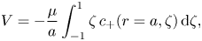 \begin{equation} V ={-}\frac{\mu}{a} \int_{{-}1}^1 \zeta \, c_+ (r=a, \zeta) \, \mathrm{d} \zeta , \end{equation}
where we have used integration by parts and introduced the change of variable  $\zeta = \cos \theta$. Correspondingly, the induced phoretic velocity is given by the first moment of concentration (Michelin, Lauga & Bartolo Reference Michelin, Lauga and Bartolo2013).
It is worth noting that an analytical approach bypassing the need for solving explicitly the Laplace equation to determine the phoretic speed has been proposed (Lammert, Crespi & Nourhani Reference Lammert, Crespi and Nourhani2016). The method permits determination of the induced phoretic speed for an arbitrary distribution of surface activity, provided that the solution of the auxiliary problem for a passive particle is known. However, to the best of our knowledge, the solution to the auxiliary problem for a sphere translating near a no-slip disk embedded in a planar interface separating two fluid media has not been derived so far, even in the simplest point-particle limit. It would be of interest to probe the applicability and pertinency in a subsequent work in which the solution of the auxiliary problem will be derived systematically.
4.2. Leading-order contribution to the phoretic velocity
At this point, we have derived the solution of the diffusion equation for a point-source singularity acting on the symmetry axis of a finite-sized disk resting on a fluid–fluid interface. We will next make use of this solution to determine the induced phoretic velocity of an active colloidal particle with isotropic surface activity. To calculate the leading-order contribution, we restrict ourselves to the point-particle approximation, which is valid when  $a \ll h$.
The image solutions derived above and given by (3.20) satisfy exactly the boundary conditions prescribed at the surface of the disk and at the fluid–fluid interface. However, they disturb the constant flux condition imposed at the surface of the active particle. To overcome this shortcoming, a series of images needs to be incorporated so as to satisfy the boundary conditions in an alternative manner up to a desired accuracy. The next-order contribution to the concentration field consists of an axisymmetric source dipole
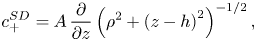 \begin{equation} c_+^{SD} = A \, \frac{\partial}{\partial z} \left( \rho^2 + \left(z-h\right)^2 \right)^{-{1}/{2}} , \end{equation}
with
 \begin{equation} A ={-}\frac {a^3}{2} \lim_{(\rho, z) \to (0, h)} \frac {\partial c_+^*}{\partial z} . \end{equation}
In this way, the boundary conditions are satisfied up to  ${O} ( \epsilon ^3 )$ at both the particle surface and the interface. Specifically,
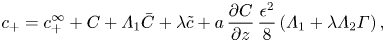 \begin{gather} c_+ = c_+^\infty + C + \varLambda_1 \bar{C} + \lambda \tilde{c} + a \,\frac{\partial C}{\partial z}\, \frac{\epsilon^2}{8} \left(\varLambda_1 + \lambda \varLambda_2 \varGamma \right) , \end{gather}
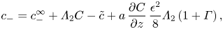 \begin{gather}c_- = c_-^\infty + \varLambda_2 C - \tilde{c} + a \, \frac{\partial C}{\partial z}\, \frac{\epsilon^2}{8} \varLambda_2 \left( 1 + \varGamma \right) , \end{gather}
where we have defined  $\bar {C} (\rho, z) = C(\rho, -z)$. Furthermore,
  $\varGamma$ is obtained so as to fulfil the constant flux boundary condition imposed at the surface of the active particle to
  ${O} ( \epsilon ^3 )$. It is given explicitly by
 \begin{equation} \varGamma = \frac{2}{\rm \pi} \left( \frac{Rh \left( R^2-h^2 \right)}{\left( R^2+h^2 \right)^2} + \arctan \left( \frac{R}{h} \right) \right) . \end{equation}
Then, by making use of (4.6) providing the induced phoretic velocity, we obtain
 \begin{equation} V =\frac{\mu Q}{D_+}\,\frac{\epsilon^2}{1+\lambda\ell} \left( \frac{1-\lambda\ell}{4} + \lambda\ell\,{\rm J}(\xi) \right) + {O} ( \epsilon^3 ) , \end{equation}
wherein  $\xi = h/R$ and
 \begin{equation} {\rm J}(\xi) = \frac{1}{\rm \pi} \left( \frac{\xi \left( 1-\xi^2 \right)}{\left( 1+\xi^2 \right)^2 }+ \arctan ( \xi^{{-}1} ) \right) \end{equation}
is a monotonically decreasing function of  $\xi$ varying between
  $1/2$ and 0. In the limit
  $\xi \ll 1$, we obtain
 \begin{equation} V =\frac{\mu Q}{4D_+} \, \epsilon^2 \left( 1 - \frac{16}{3{\rm \pi}} \, \lambda \varLambda_2 \xi^3 \right) + {O} ( \xi^5 ) . \end{equation}
This result is valid in the far-field limit such that  $\epsilon \ll 1$. In particular, we recover the leading-order far-field contribution to the induced phoretic velocity in the limit of an infinitely extended no-slip wall as obtained originally by Ibrahim & Liverpool (Reference Ibrahim and Liverpool2015). This result has later been generalised by Yariv (Reference Yariv2016) for both remote and near-contact configurations using a first-order kinetic model of solute absorption.
Figure 4 shows in a semi-logarithmic scale the evolution of the scaled phoretic velocity as given by (4.11) as a function of  $\xi = h/R$. Results are presented for six different values of
  $\lambda \ell = ( \eta _+/\eta _- ) / ( c_+^\infty / c_-^\infty )$ that span the most likely values for fluid–fluid interfaces to be expected for a wide range of practical situations. The limiting case
  $\lambda \ell \to 0$ corresponds to the situation of a liquid–solid interface where the solid phase acts as a stiff medium (
 $\eta _- \to \infty$) with vanishing solubility (
 $\ell =0$). The case of a liquid–gas interface without evaporation of the solute (active particle immersed in the liquid phase) would correspond to
  $\lambda \gg 1$, yet
  $\lambda \ell \to 0$ because of vanishing solubility. For instance, for an air–water interface, it is estimated that
  $\lambda \sim 50$ and
  $\ell \sim 10^{-2}\text {--} 10^{-1}$ (Battino, Rettich & Tominaga Reference Battino, Rettich and Tominaga1983) such that
  $\lambda \ell \sim 0.5\text {--}5$. For a liquid–liquid interface, such as water–decane, values of the order
  $\lambda \sim ~1$ and
  $\ell \sim 1$ are expected (Ju & Ho Reference Ju and Ho1989).
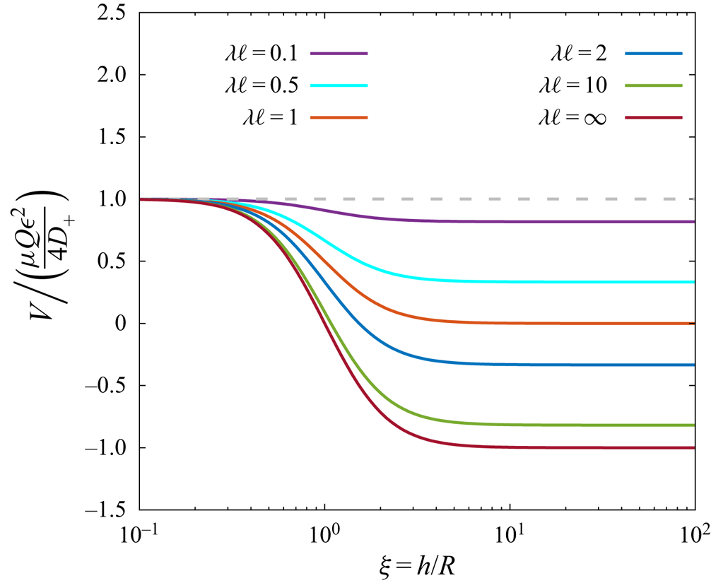
Figure 4. Variation of the scaled induced phoretic velocity near a finite-sized disk resting on a fluid–fluid interface as given by (4.11) versus the dimensionless number  $\xi = h/R$ for various values of
  $\lambda \ell$. The horizontal dashed line corresponds to the situation of an infinite wall such that
  $\lambda \ell \to 0$.
The scaled velocity amounts to its maximum value as  $\xi \to 0$, and decreases monotonically with
  $\xi$ to reach the value corresponding to a fluid–fluid interface given by
 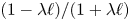 $( 1-\lambda \ell ) / ( 1+\lambda \ell )$ in the limit
  $\xi \to \infty$. The active particle is found to be repelled from the interface or attracted to it, depending on the sign of the phoretic mobility
  $\mu$ and the flux
  $Q$, as well as the values of the dimensionless parameters
  $\lambda \ell$ and
  $\xi$. Under some circumstances, the particle remains in a stationary hovering state in which it acts as a micropump.
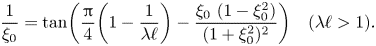
The phoretic speed keeps the same sign over the whole range of values of  $\xi$ when
  $\lambda \ell \le 1$. Correspondingly, the particle is repelled from the interface for
  $\mu Q > 0$ and attracted for
  $\mu Q < 0$. This behaviour is analogous to what has been reported earlier for diffusiophoresis near an infinite no-slip wall (Ibrahim & Liverpool Reference Ibrahim and Liverpool2015; Yariv Reference Yariv2016). In contrast to that, the induced speed can vanish eventually, and changes sign when
  $\lambda \ell > 1$. By equating (4.11) to zero and solving for
  $\xi$, we find that the phoretic velocity vanishes at a unique value
  $\xi = \xi _0$ given by the solution of
 \begin{equation} \frac{1}{\xi_0} = \tan
\biggl(\frac{\rm \pi}{4} \biggl( 1 - \frac{1}{\lambda\ell} \biggr) -
\frac{\xi_0\ (1-\xi_0^2)}{(1+\xi_0^2)^2}\biggr) \quad (\lambda\ell > 1) .
\end{equation}
\begin{equation} \frac{1}{\xi_0} = \tan
\biggl(\frac{\rm \pi}{4} \biggl( 1 - \frac{1}{\lambda\ell} \biggr) -
\frac{\xi_0\ (1-\xi_0^2)}{(1+\xi_0^2)^2}\biggr) \quad (\lambda\ell > 1) .
\end{equation}
Accordingly, for  $\lambda \ell > 1$, the active particle is repelled from the interface if
  $\mu Q ( \xi -\xi _0 ) < 0$ and attracted to it if
  $\mu Q ( \xi -\xi _0 ) > 0$.
For  $\lambda \ell \gg 1$, we obtain the scaling relation
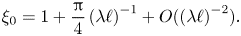 \begin{equation} \xi_0 = 1 + \frac{\rm \pi}{4} \left(\lambda\ell\right)^{{-}1} + {O} ( \left(\lambda\ell\right)^{{-}2} ) . \end{equation}
In particular, it follows from (4.6) that the induced phoretic velocity near a fluid–fluid interface is obtained as
 \begin{equation} V =\frac{\mu Q}{4 D_+}\,\frac{1-\lambda\ell}{1+\lambda\ell} \, \epsilon^2 + {O} ( \epsilon^3 ) . \end{equation}
 In many physically relevant situations of liquid–liquid interfaces,  $\lambda \ell$ remains of the order of or less than 1, suggesting that the sign of the induced phoretic speed is determined solely by the product
  $\mu Q$ as discussed above. In contrast to that, for gas–liquid interfaces,
  $\lambda \ell$ might under most circumstances exceed 1, so that that the sign of the phoretic mobility is additionally dependent on the ratio
  $\xi$.
In figure 5 we present the variation of  $\xi _0$ by solving numerically (4.14) using standard computational techniques. We remark that
  $\xi _0$ approaches infinity asymptotically as
  $\lambda \ell \to 1$, and decreases monotonically before reaching a minimum value of 1 as
  $\lambda \ell \to \infty$. The linear scaling behaviour predicted by (4.15) is shown by using a log-log scale in the inset.


Up to now, we have obtained the leading-order contribution to the phoretic velocity of an active isotropic colloid suspended near a circular disk of finite size settling on a surface separating two fluids. A power series solution for the induced phoretic velocity can in principle be obtained perturbatively by considering additional singular fields in the concentration field. However, due to their complexity and the intricate form of the image solution, accounting for additional singularities is rather delicate and laborious.
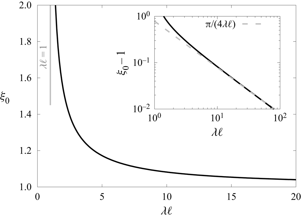
Figure 6 shows a comparison of the scaled phoretic velocity near a fluid–fluid interface as obtained by means of bipolar coordinates (symbols) reported recently by Malgaretti et al. (Reference Malgaretti, Popescu and Dietrich2018) and the far-field expression given by (4.16). Results are plotted versus the dimensionless ratio  $\epsilon$ of particle radius to distance from the interface for
  $\lambda \ell = 0.2$ (blue) and
  $\lambda \ell = 5$ (red), while the viscosity ratio is kept
  $\ell = 1$. Good agreement is obtained between the exact analytical solution and the simplistic far-field expression derived in the present work. In particular, both approaches capture the same underlying physical behaviour on whether the particle moves towards the interface or away from it. As shown in the inset, the far-field approach leads to a relative percentage error smaller than
  $10\,\%$ when
  $\epsilon < 0.5$. The error increases monotonically as the particle gets closer to the interface, for
  $\epsilon = 0.9$ reaching approximately
  $20\,\%$ for
  $\lambda \ell = 5$ and
  $40\,\%$ for
  $\lambda \ell = 0.2$.
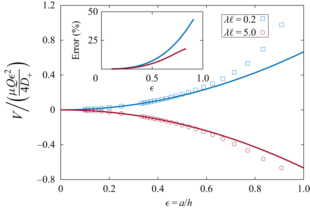
Figure 6. Scaled induced phoretic velocity near an infinitely extended fluid–fluid interface (in the absence of the disk) as a function of the dimensionless particle size  $\epsilon = a/h$ for two different values of
  $\lambda \ell$. Symbols represent the exact results obtained using bipolar coordinates (Malgaretti et al. Reference Malgaretti, Popescu and Dietrich2018), and solid lines indicate the far-field solution derived in the present work given by (4.16). Here, the viscosity ratio between the two media is
  $\ell = 1$. The inset shows the relative percentage error, which is of the order
  $\propto \epsilon ^3$.
To validate our analytical approximation that is carried out in the limit of small sphere sizes,  $\epsilon \ll 1$, we solved the diffusion problem numerically for a wide range of sizes of a truly extended sphere near a finite-sized no-slip disk resting on an interface between two fluids. We solve the diffusion equation with an axisymmetric boundary element method using the Green functions from BEMLIB (Pozrikidis Reference Pozrikidis2002). We discretised the sphere, the disk and the boundary with 800 collocation points each, and verified consistently that halving the number of discretisation points led to errors
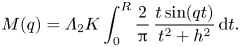
  $\ll 1\,\%$. For each set of parameters, we evaluated the first moment of concentration that appears in (4.6). The results for the scaled induced phoretic velocity are shown in figure 7 for the case
  $\lambda \ell =1$ and a range of values for the dimensionless ratio
  $\xi = h/R$. Excellent agreement between analytical results and boundary element calculations is found for small values of
  $\epsilon$. The relative errors are below 3 % for
  $\epsilon < 0.5$ and grow monotonically as
  $\epsilon$ increases, reaching approximately 30 % for
  $\epsilon = 0.9$; see inset of figure 7. On that account, the point-particle approximation employed in the present work, despite its simplicity, shows its robustness in predicting the overall behaviour of the system under investigation.
Figure 7. Scaled induced phoretic velocity near a finite-sized no-slip disk embedded in a fluid–fluid interface separating two fluid media of the same dynamic viscosity and solubility such that  $\lambda \ell = 1$. Results are plotted against the dimensionless ratio
  $\epsilon = a/h$ for various values of dimensionless parameter
  $\xi = h/R$. Symbols represent the numerical results obtained using the boundary element method, and solid lines show the approximate analytical solution derived in the present work given by (4.11).
Finally, it is worth noting that due to the gradient of the chemical species at the interface, the induced Marangoni stresses may drive a fluid flow, resulting in a hydrodynamic drift that pushes the active colloid towards or away from the interface, depending on how the activity is modified by surface tension (Domínguez et al. Reference Domínguez, Malgaretti, Popescu and Dietrich2016). We now assume that that the surface tension of the fluid–fluid interface depends linearly on the local concentration of solute species via
 \begin{equation} \gamma (\boldsymbol{r}) = \gamma_0 - \kappa \left( c(r=0,z) - c_+^\infty \right) , \end{equation}
with  $\gamma _0$ denoting the equilibrium surface tension and
  $\kappa$ of dimension [M][L]
 $^3$[T]
 $^{-2}$. On the one hand, the hydrodynamic drift velocity resulting from Marangoni stresses is expected to scale as
 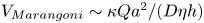 $V_{Marangoni} \sim \kappa Q a^2 / ( D \eta h )$ (Domínguez et al. Reference Domínguez, Malgaretti, Popescu and Dietrich2016). On the other hand, the self-induced phoretic velocity derived in the present work is
 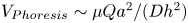 $V_{Phoresis} \sim \mu Q a^2 / ( D h^2 )$. By assuming that
  $\kappa h / ( \mu \eta ) \ll 1$ so that
 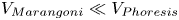 $V_{Marangoni} \ll V_{Phoresis}$, the Marangoni effect becomes subdominant to phoretic effects. The contribution to the drift velocity due to Marangoni stresses could be quantified in terms of the system properties and is worth investigating in a future work.
5. Conclusions
To summarise, we have presented a far-field analytical theory addressing the axisymmetric autophoretic motion of an isotropic active particle suspended in a viscous Newtonian fluid medium near a rigid disk embedded in a planar fluid–fluid interface. We have formulated the solution for the concentration field induced by a point-source singularity as a standard mixed-boundary-value problem, which we have then reduced to a classical Abel integral equation amenable to analytical inversion. By making use of the Lorentz reciprocal theorem, we have obtained an analytical expression for the leading-order far-field contribution to the induced phoretic velocity, thereby elevating the need to solve for the hydrodynamic flow field explicitly.
On the one hand, we have shown that for  $\lambda \ell < 1$, the induced velocity normal to the interface depends solely on the phoretic mobility and chemical activity, and is found to be independent of the system geometrical properties. Specifically, the case
  $\mu Q > 0$ corresponds to repulsion from the interface, while
  $\mu Q < 0$ corresponds to attraction. On the other hand, we have shown that for
  $\lambda \ell > 1$, there exists a size ratio
  $\xi _0$ for which the active particle reaches a steady motionless hovering state above the interface. Beyond this state, the active particle is found to be repelled from (attracted to) the interface, depending on whether
  $\mu Q ( \xi - \xi _0 )$ is negative (positive).
From an experimental standpoint, we believe that potentially, our theoretical predictions could be verified in real-space experiments on active colloids. In the present work, we focused our attention on the situation in which the disk is physically adhered to the interface such that its motion is fully restricted. It is well known that at fluid–fluid interfaces with very large surface tension, contact-line pinning typically constrains the motion of embedded objects pronouncedly (Chisholm & Stebe Reference Chisholm and Stebe2021). With the possibility of exploiting this effect, an experimental realisation of our set-up for a rigid disk resting on an interface can be achieved. On the other hand, the isotropic active colloid is assumed to be wholly immersed in one of the two fluids without establishing physical contact with the interface. Under controlled experimental conditions, the self-induced swimming velocity can then be measured and quantified in terms of the set-up geometry and the chemophysical properties of the interface.
The present analytical developments are based on a far-field description of the phoretic and hydrodynamic fields. They rely on the assumption that the active particle is small relative to its distance from the interface. As a perspective, it would be of interest to assess the appropriateness and accuracy of the point-particle approximation employed in this work by direct comparison with a fully resolved numerical boundary integral equation for the hydrodynamic field. In addition, it would be worthwhile to extend our analytical approach to address the behaviour of an active Janus particle partially coated with a catalytic cap promoting a chemical reaction on only a portion of its surface.
For an accurate representation of an extended active particle of finite radius, higher-order reflections in the phoretic and hydrodynamic fields should be accounted for further. This can be achieved by including additional singularities so as to satisfy the boundary conditions imposed at the particle and at the interfaces iteratively using the classical method of successive images. Also, an exact solution of the phoretic and hydrodynamic problems can be obtained alternatively based on the eigensolution expansion of the Laplace equation using the system of bipolar coordinates. These aspects constitute an interesting extension of the present problem for future investigations.
Funding
We acknowledge support from the Max Planck Center Twente for Complex Fluid Dynamics, the Max Planck School Matter to Life, and the MaxSynBio Consortium, which are funded jointly by the Federal Ministry of Education and Research (BMBF) of Germany and the Max Planck Society. This work was supported by Slovenian Research Agency (A.V., grant no. P1-0099).
Declaration of interests
The authors report no conflict of interest.
Appendix A. Expressions of integrals  $\mathcal {L}_m^n$

The (improper) integrals given by (3.10) in the main body of the paper are convergent and can be evaluated analytically. It can be shown that for  $n = 0$ (Abramowitz & Stegun Reference Abramowitz and Stegun1972; Gradshteyn & Ryzhik Reference Gradshteyn and Ryzhik2014),
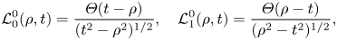 \begin{equation} \mathcal{L}_0^0 (\rho, t) = \frac{\varTheta (t - \rho)}{( t^2-\rho^2 )^{{1}/{2}}} , \quad \mathcal{L}_1^0 (\rho, t) = \frac{\varTheta (\rho - t)}{( \rho^2 - t^2 )^{{1}/{2}}} , \end{equation}
with  $\varTheta (\cdot )$ denoting Heaviside's step function. Using the fact that
  ${\rm J}_0'(x) = -{\rm J}_1(x)$ (where a prime denotes a derivative with respect to the argument) together with the differentiation and integration properties of trigonometric functions, it can be shown further that
 \begin{equation} \mathcal{L}_0^1 (\rho, t) = \frac{t \, \mathcal{L}_1^0 (\rho, t)}{\rho} , \quad \mathcal{L}_1^1 (\rho, t) = \frac{1 - t \, \mathcal{L}_0^0 (\rho, t)}{\rho} . \end{equation}
Appendix B. Evaluation of the indefinite integral in (3.27)
In this appendix, we show using the residue theorem in complex analysis that
 \begin{equation} \operatorname{Im} \left\{ \int_0^\infty f(z) \, \mathrm{d} z \right\} = \frac{\rm \pi}{2} ( a^2+(b+c)^2 )^{-{1}/{2}} , \end{equation}
where
 \begin{equation} f(z) = z ( z^2 + c^2 )^{{-}1} ( a^2 + (b-{\rm i}z)^2 )^{-{1}/{2}} \end{equation}
is a complex analytical function defined in the upper half-plane. In addition,  $(a,b,c) \in \mathbb {R}_+^3$. Since
  $f(-z) = -\overline {f(z)}$, where the bar denotes the complex conjugate, and
  $\operatorname{Im} \{ z \} = (z-\bar{z})/(2i), $ it follows that
 \begin{equation} \operatorname{Im} \left\{ \int_0^\infty f(z) \, \mathrm{d} z \right\} = \frac{1}{2{\rm i}} \int_{-\infty}^\infty f(z) \, \mathrm{d} z . \end{equation}
 To evaluate the improper integral on the right-hand side of (B3), we employ the usual approach by choosing a closed integration contour  $\gamma = \gamma _1 + \gamma _2$, with
  $\gamma _1$ denoting the linear path along the real axis in the interval
  $[-R,R]$, and
  $\gamma _2$ the circular path of radius
  $R$. Accordingly,
 \begin{equation} \oint_{\gamma} f(z) \, \mathrm{d} z = 2{\rm i}{\rm \pi} \sum \operatorname{Res} (f, z_i) . \end{equation}
 By setting  $z = R {\rm e}^{{\rm i}\theta }$ with
  $\theta = [0,{\rm \pi} ]$, it follows that
  $\mathrm {d} z = {\rm i}R {\rm e}^{{\rm i}\theta } \, \mathrm {d} \theta$. Then the integral along the circular path
  $\gamma _2$ can be evaluated asymptotically as
 \begin{equation} \int_{\gamma_2} f(z) \, \mathrm{d} z = 2R^{{-}1} + {O} ( R^{{-}2} ) \xrightarrow[R\to\infty]{} 0 . \end{equation}
 Thus the contour integration reduces to that along  $\gamma _1$, leading when taking the limit
  $R\to \infty$ to
 \begin{equation} \int_{-\infty}^\infty f(z) \, \mathrm{d} z = 2{\rm i}{\rm \pi} \operatorname{Res} (f, {\rm i}c) = {\rm i}{\rm \pi} ( a^2 + (b+c)^2 )^{-{1}/{2}} . \end{equation}


 Open access