


1. Introduction
Wave–current interaction is a classic oceanic phenomenon that has been studied for several decades. Most previous studies assumed irrotational flows and adopted the fully nonlinear potential flow theory (Dommermuth & Yue Reference Dommermuth and Yue1988; Wang, Ma & Yan Reference Wang, Ma and Yan2018). However, currents in the natural environment may contain a certain degree of shear in both vertical and horizontal directions, and the effects of vorticity on ocean surface waves cannot always be ignored. For example, wind-generated currents may exhibit a strong shear near the free surface (Swan, Cummins & James Reference Swan, Cummins and James2001; Kharif et al. Reference Kharif, Giovanangeli, Touboul, Grare and Pelinovsky2008), and benthic turbulent currents show a strong shear close to the sea bottom (Kemp & Simons Reference Kemp and Simons1982). Peregrine (Reference Peregrine1976) and Jonsson (Reference Jonsson1990) provided comprehensive reviews on various theoretical studies of wave–current interactions.
In most previous studies, only two-dimensional (2D) currents (on the vertical plane) with a linear profile in the water column (i.e. a constant shear and constant horizontal vorticity) have been considered. Stokes wave-type perturbation expansion method has often been used for studying weakly nonlinear waves interacting with such a current (Tsao Reference Tsao1959; Brevik Reference Brevik1979; Kishida & Sobey Reference Kishida and Sobey1989; Pak & Chow Reference Pak and Chow2009). On the other hand, Dalrymple (Reference Dalrymple1974) obtained finite-amplitude wave solutions numerically using a Fourier series expansion method based on the stream function formulation. The boundary integral equation method has also been widely employed for studying finite-amplitude waves on currents with a constant shear. For example, Simmen & Saffman (Reference Simmen and Saffman1985) and Teles Da Silva & Peregrine (Reference Teles Da Silva and Peregrine1988) obtained periodic wave solutions in deep and finite water depths, whereas Vanden-Broeck (Reference Vanden-Broeck1994) presented steep solitary wave solutions in finite water depth. More recently, Moreira & Chacaltana (Reference Moreira and Chacaltana2015) studied wave blocking and breaking in deep water, induced by currents of constant horizontal vorticity, through a fully nonlinear boundary integral method. Ellingsen (Reference Ellingsen2016) found analytical solutions for oblique incident linear waves on vertically linearly sheared currents and concluded that waves are rotational and the vortex lines are gently shift and twist as the wave passes. Francius & Kharif (Reference Francius and Kharif2017) studied numerically the stability of finite-amplitude waves in finite water depth on vertically sheared currents of constant horizontal vorticity. In the shallow-water regime, based on a strongly nonlinear and weakly dispersive depth-integrated equation, Choi (Reference Choi2003) found solutions for solitary waves riding on currents with a linear profile in the water column. Duan et al. (Reference Duan, Wang, Zhao, Ertekin and Yang2018) also obtained similar results using the Green–Naghdi equations.
Several studies have been performed to examine the effects of currents with different profiles in the water column on wave propagation. Using a weakly nonlinear stream function theory, Benjamin (Reference Benjamin1962) studied solitary waves on currents with arbitrary vorticity distribution. On the other hand, Dalrymple (Reference Dalrymple1977) used the Dubreil–Jacotin transformation technique to investigate finite-amplitude waves on currents with a 1/7 power law profile in the water column. Swan & James (Reference Swan and James2000) derived analytical solution for second-order Stokes waves on depth-varying currents, whose strength was weak relative to wave celerity. The vertical profile of the current field was assumed to be a third-degree polynomial and, thus, the vorticity profile was a second-degree polynomial. Nwogu (Reference Nwogu2009) proposed a boundary integral method to study finite-amplitude waves on current with an exponential profile in deep water, in which the current field was assumed to be horizontally uniform and always in steady state. By dividing the water column into several layers and assuming the current field to be linearly varying in each vertical layer, a piecewise-linear approximation method was adopted by Zhang (Reference Zhang2005) for solving the Rayleigh equations. The same method was also used by Smeltzer & Ellingsen (Reference Smeltzer and Ellingsen2017) to extend Ellingsen's (Reference Ellingsen2016) work to obliquely incident waves interacting with currents with an arbitrary angle. Most recently, Chen & Basu (Reference Chen and Basu2021) proposed a numerical method for computing steady-state large-amplitude waves on depth-varying currents based on a stream function formulation. The effects of vertically linearly sheared currents on the highest waves were discussed.
In the large-scale ocean modelling community, the concept of radiation stress (Longuet-Higgins & Stewart Reference Longuet-Higgins and Stewart1960, Reference Longuet-Higgins and Stewart1961), which is the excess momentum flux averaged over a wave period and total water depth, has been used to calculate the wave effects on currents. The radiation stress concept has been successfully employed to explain various physical processes such as wave setup/setdown, surf beat, and longshore currents. For ocean circulation modelling in three dimensions, the depth-dependent radiation stress can be derived by taking the wave-average of the three-dimensional (3D) flow momentum equation without depth integration (Mellor Reference Mellor2003, Reference Mellor2008). This formulation has been implemented in the COAWST model for surf zone and rip-current applications (Kumar et al. Reference Kumar, Voulgaris, Warner and Olabarrieta2012). Alternatively, the vortex force formalism (Leibovich Reference Leibovich1980) has been applied recently to describe wave–current interaction in ocean circulation models. For example, McWilliams, Restrepo & Lane (Reference McWilliams, Restrepo and Lane2004) derived a multi-scale asymptotic theory for the evolution and interaction of currents and surface gravity waves in finite depth, and the current was assumed to be very weak compared with wave celerity. The vortex force formalism was also adopted in surf zone circulation models in computing the effects of waves on currents (Uchiyama, McWilliams & Shchepetkin Reference Uchiyama, McWilliams and Shchepetkin2010; Kumar et al. Reference Kumar, Voulgaris, Warner and Olabarrieta2012). For the effects of the current on waves, Kirby & Chen (Reference Kirby and Chen1989) obtained the frequency dispersion relation of linear waves on weak currents of arbitrary profiles in finite depth, using a perturbation approach, which was the extension of Skop (Reference Skop1987). Following Kirby & Chen (Reference Kirby and Chen1989), Banihashemi, Kirby & Dong (Reference Banihashemi, Kirby and Dong2017) and Banihashemi & Kirby (Reference Banihashemi and Kirby2019) derived approximated wave action conservation and wave action flux velocity in strongly sheared mean flows. Li & Ellingsen (Reference Li and Ellingsen2019) presented a framework for modelling linear waves on currents of arbitrary vertical profiles where bathymetry and ambient currents varied slowly in horizontal directions.
For coastal applications, a majority of wave–current models can be classified as depth-integrated models (e.g. shallow-water equation, Boussinesq-type models, and non-hydrostatic models), in which the dimension of the problem is reduced by one through integrating the mass and momentum equations over the water column and reinforcing the boundary conditions on the sea bottom and the free surface. A literature review on the development of depth-integrated models can be found in Yang & Liu (Reference Yang and Liu2020) (referred to as YL20 herein). In the Boussinesq-type models, the current is usually approximated as the depth-averaged velocity (Yoon & Liu Reference Yoon and Liu1989; Chen et al. Reference Chen, Madsen, Schäffer and Basco1998; Zou et al. Reference Zou, Hu, Fang and Liu2013). Although several attempts were made to incorporate vorticity effects in Boussinesq-type models (Shen Reference Shen2001; Castro & Lannes Reference Castro and Lannes2014; Son & Lynett Reference Son and Lynett2014), only restricted current profiles (or vorticity strengths) can be used. Moreover, these models can only be applicable in a relatively shallow-water regime. The so-called non-hydrostatic models assume depth-uniform horizontal velocity in each vertical layer. Thus, a large number of vertical layers are necessary to describe current with strong local shear, which may significantly increase the computational cost.
More recently, Touboul et al. (Reference Touboul, Charland, Rey and Belibassakis2016) extended the mild-slope equation to study linear waves on a background current, which was slowly varying in the horizontal direction and was linearly sheared in the vertical direction. However, the wave components were still assumed to be irrotational, which is not true because flows are 3D (Ellingsen Reference Ellingsen2016). It is essentially a one-way wave–current model, taking only the influences of background current on linear waves into account. Similar models were derived by Belibassakis et al. (Reference Belibassakis, Simon, Touboul and Rey2017) to study the effects of linearly sheared currents over general bathymetry. Furthermore, a coupled-mode model was developed by Touboul & Belibassakis (Reference Touboul and Belibassakis2019) to study the effects of a vertically sheared steady-state background current field on the propagation of linear waves, which is a one-way wave–current interaction extension of the model derived in Belibassakis & Touboul (Reference Belibassakis and Touboul2019). Similarly, Beyer (Reference Beyer2018) extended the deep-water Green–Naghdi equations to consider vertically sheared currents, in which the horizontal velocity was approximated by an exponential function for simulating deep-water waves. However, a decay parameter in the exponential function needs to be predetermined, which was chosen to be the (peak) wavenumber. The background current field was restricted to be horizontally slowly varying and cannot be modified by waves.
YL20 presented a hierarchy of depth-integrated wave–current models, in which the vertical profile of the horizontal velocity was approximated as a series of polynomials. As the total horizontal velocity (the combination of current and wave velocities) was approximated in YL20, a higher degree polynomial must be used to simulate deeper-water waves and/or currents with complex profiles in the water column. For example, in a very shallow-water regime, the wave orbital velocity is almost uniform in the water column, but the current could have an exponential profile in the water column. Then, in YL20's approach, models of higher approximation (higher degree polynomial) must be used to approximate the current profile properly. To overcome this shortcoming, in this paper a new approach is proposed so that the vertical profile of the current can be adopted in the model without further approximation. The new approach decomposes the solutions for the horizontal velocity into two unknown components: the first component adopts the vertical profile of the prescribed steady-state current in the  $\sigma$ coordinate, which contains the unknown free surface elevation. The constraint on the first solution component is that, in the absence of waves, it reduces to the prescribed steady-state current field. The second component of the horizontal velocity is approximated in the polynomial form in a similar way as shown in YL20. Euler equations and boundary conditions are used to constrain the total solutions.
Using different weighting functions in the weighted residual methods, two kinds of depth-integrated wave–current models were developed in YL20, that is, the Galerkin model and the subdomain model. It was shown in YL20 that the subdomain model is superior to the Galerkin model in terms of various wave properties, and the numerical implementation of the subdomain model with any degree of polynomial approximation is also more straightforward. Thus, in this paper, only the subdomain model ( $SK$) is discussed for brevity, in which the vertical structure of the horizontal velocity is the (
 $K-1$) degree polynomial and
  $K$ also represents the number of velocity variables.
This paper is organized as follows. The derivation of the mathematical model from 3D Euler equations to the depth-integrated two-dimensional horizontal (2DH) equations is presented in § 2. As the present model is built upon YL20, only the details of the new approach on incorporating the prescribed current field in the water column are highlighted. A theoretical analysis of frequency dispersion properties of linear waves on vertically sheared currents is conducted in § 3, in which the accuracy of the models is discussed by considering waves in different relative water depths, current directions, current intensities, and current vertical profiles. Section 4 introduces the numerical applications of the mathematical models. The present models are validated with laboratory experiments of finite-amplitude waves propagating over sheared currents for free surface elevations and horizontal velocities in one-dimensional horizontal (1DH) space. Numerical validations and investigations are then conducted for nonlinear deep-water and intermediate-water waves on currents of different profiles. In the shallow-water regime, solitary waves of different nonlinearity on vertically arbitrarily sheared current are also studied. The resulting wave properties, e.g. free surface elevations, velocity field, and time-averaged velocity field are discussed accordingly. Two applications of present models on wave propagation and transformation over sheared currents in 2DH space are also presented in § 4. Finally, conclusions are drawn in § 5. For completeness, some of the validations of present models against experimental data for wave transformation in 2DH space without currents and wave–current interactions in 1DH space are included in the supplementary materials available at https://doi.org/10.1017/jfm.2022.42.
2. Derivation of mathematical models
In this study, we assume that water is incompressible and inviscid, and the free surface flow is governed by the Euler equations. When waves are absent, a steady-state current field is assumed to exist, with a prescribed velocity field and corresponding free surface elevation distribution. As waves propagate into the current field, the resulting wave–current interaction problem is the solution of the Euler equations and boundary equations. The derivation of the 2DH mathematical model is briefly presented in the following section.
2.1. Governing equations
Following YL20, a  $\sigma$-coordinate transformation is introduced to map the water column from
  $[-h, \eta ]$ in the Cartesian coordinate to a fixed range
  $[0, 1]$ in the
  $\sigma$-coordinate. This transformation is defined as follows:
 \begin{equation} t=t^*, \quad x_i=x_i^*, \quad \sigma=\frac{z^*+h}{h+\eta}=\frac{z^*+h}{H}, \end{equation}
where  $t^*$ is the time,
  $x^*_i \ (i=1,2)$ are the horizontal coordinates in the Cartesian coordinate with
  $z^*$-axis pointing upwards, and the horizontal plane is located on the still water level. In the following we omit asterisks for brevity. The independent variables in the
  $\sigma$-coordinate are
  $(x_i,\sigma,t)$, where
  $\sigma$ is a function of the free surface elevation
  $\eta (x_i,t)$ and sea bottom configuration
  $h (x_i)$. The total water depth is denoted by
  $H=h+\eta$.
The governing equations and boundary conditions in the  $\sigma$-coordinate have been presented in YL20; they are shown here for completeness and clarity:
 \begin{gather} \frac{\partial u_i}{\partial x_i}+\frac{\partial u_i}{\partial \sigma}\sigma_{x_i}+\frac{\partial w}{\partial \sigma}\sigma_z=0 , \end{gather}
 \begin{gather} \frac{\partial u_i}{\partial t}+\frac{\partial u_i}{\partial \sigma}\sigma_t+u_j\left(\frac{\partial u_i}{\partial x_j}+\frac{\partial u_i}{\partial \sigma}\sigma_{x_i}\right)+w\frac{\partial u_i}{\partial \sigma}\sigma_z ={-}\frac{1}{\rho}\left(\frac{\partial p}{\partial x_i}+\frac{\partial p}{\partial \sigma}\sigma_{x_i}\right) , \end{gather}
 \begin{gather} \frac{\partial w}{\partial t}+\frac{\partial w}{\partial \sigma}\sigma_t+u_j \left(\frac{\partial w}{\partial x_j}+\frac{\partial w}{\partial \sigma}\sigma_{x_i}\right)+w \frac{\partial w}{\partial \sigma}\sigma_z ={-}\frac{1}{\rho}\frac{\partial p}{\partial \sigma}\sigma_z-g. \end{gather}
 \begin{gather} p|_s=0, \quad \sigma=1,\end{gather}
 \begin{gather} \frac{\partial \eta}{\partial t}+u_i|_s\frac{\partial \eta}{\partial x_i}=w|_s, \quad \sigma=1,\end{gather}
 \begin{gather} u_i|_b\frac{\partial h}{\partial x_i}+w|_b=0, \quad \sigma=0, \end{gather}
where  $u_i$ and
  $w$ are the horizontal and vertical velocity components in the
  $\sigma$ coordinate, respectively, and
  $p$ is the pressure field. The total fluid domain is bounded by an impermeable bottom,
  $z=-h(x_i)$ or
  $\sigma =0$, and the free surface,
  $z=\eta (x_i,t)$ or
  $\sigma =1$. The subscripts
  $s$ and
  $b$ appeared in the boundary conditions denote that the physical variables are evaluated at the free surface and the sea bottom, respectively. Here
  $\rho$ is the density of water and
  $g$ is the gravitational acceleration. Finally,
  $\sigma _{t}$,
  $\sigma _{x_i}$ and
  $\sigma _{z}$ are the partial derivatives of
  $\sigma$ with respect to time, horizontal and vertical coordinates, respectively, and they can be obtained by chain rule as follows:
 \begin{equation} \sigma_{t}={-}\sigma\frac{1}{H}\frac{\partial H}{\partial t}, \quad \sigma_{x_i}=\frac{1}{H}\left(\frac{\partial h}{\partial x_i}-\sigma\frac{\partial H}{\partial x_i}\right), \quad \sigma_{z}=\frac{1}{H}. \end{equation}
Following the same approach as in YL20, the depth-integrated continuity equation, the vertical velocity and pressure field are given directly as follows:
 \begin{gather} \frac{\partial H}{\partial t}+\frac{\partial }{\partial x_i}\int_{0}^{1}\frac{1}{\sigma_z} u_i\,\mathrm{d}\sigma=0, \end{gather}
 \begin{gather} w={-}{u_i}|_b\frac{\partial h}{\partial x_i}-\frac{1}{\sigma_z}\left[\int_0^\sigma \left( \frac{\partial u_i}{\partial x_i}+\frac{\partial u_i}{\partial \sigma}\sigma_{x_i}\right)\,\mathrm{d}\sigma\right],\end{gather}
 \begin{gather} p=\frac{1}{\sigma_z}\left[\rho g (1-\sigma)+\rho \int_\sigma^{1} \left(\frac{\partial w}{\partial t}+\frac{\partial w}{\partial \sigma}\sigma_t+u_j \left(\frac{\partial w}{\partial x_j}+\frac{\partial w}{\partial \sigma}\sigma_{x_i}\right)+w \frac{\partial w}{\partial \sigma}\sigma_z\right)\,\mathrm{d}\sigma\right]. \end{gather}
By substituting the pressure field (2.11) into (2.3), the horizontal momentum equation becomes
 \begin{align} &\frac{\partial u_i}{\partial t}+\frac{\partial u_i}{\partial \sigma}\sigma_t+u_j \left(\frac{\partial u_i}{\partial x_j}+\frac{\partial u_i}{\partial \sigma}\sigma_{x_i}\right)+w\frac{\partial u_i}{\partial \sigma}\sigma_z \nonumber\\ &\quad ={-} g\frac{\partial (H-h)}{\partial x_i}- \frac{\partial }{\partial x_i}\int_{\sigma}^{1} \frac{1}{\sigma_z}p_{nh} \,\mathrm{d}\sigma+\frac{\sigma_{x_i}}{\sigma_z}p_{nh}, \end{align}
where
 \begin{equation} p_{nh}=\frac{\partial w}{\partial t}+\frac{\partial w}{\partial \sigma}\sigma_t+u_j \left(\frac{\partial w}{\partial x_j}+\frac{\partial w}{\partial \sigma}\sigma_{x_i}\right)+w \frac{\partial w}{\partial \sigma}\sigma_z. \end{equation}
The above equations are exact.
In YL20, a trial solution,  $\tilde {u}$, is introduced as an infinite series of products of prescribed shape functions,
  $N_j(\sigma )$, and unknown functions
  $u_{i,j}(x_i, t)$, which depend on the horizontal coordinates and time, i.e.
  $\tilde {u}_i=\sum _{j=1}^{K}u_{i,j}N_j(\sigma )$. Substituting the trial solution into the horizontal momentum equation (2.12) and the depth-integrated continuity equation (2.9) and applying the weighted residual method (Finlayson Reference Finlayson2013), a system of approximated differential equations for
  $u_{i,j}$ and
  $H$ are derived.
The complexity and applicability of these models depend on the choice of shape function, weighting function and the number of truncated terms kept in the horizontal velocity approximation, namely,  $K$. For example, in the subdomain model discussed in YL20,
  $N_j(\sigma )=\sigma ^{j-1}$ is the shape function employed;
  $S2$ denotes the subdomain weighted residual method with
  $K=2$, meaning the trial solution is approximated as a linear function of
  $\sigma$. Thus, once the value of
  $K$ or the degree of the polynomial in the trial solution is decided, the ability of the model in describing the fluid horizontal velocity is restricted accordingly. Thus, in YL20 a larger truncation number
  $K$ (or higher degree polynomial) is necessary for deeper-water waves and/or currents with a complex profile in the water column. For instance, in YL20, the
  $S2$ model can only accurately describe a constantly sheared current (i.e. linear velocity profile in the water column).
To improve the wave–current models in YL20, in this paper, the interaction between waves and a prescribed arbitrarily sheared current field is formulated differently as follows. The solutions for the total horizontal velocity and total water depth are expressed as
 \begin{gather} u_i(x_i,\sigma , t)=u'_i(x_i,\sigma, t)+u^*_i(x_i,\sigma), \end{gather}
 \begin{gather}H(x_i,t)=\eta'(x_i,t)+\eta^c(x_i)+h(x_i), \end{gather}
where the total free surface elevation has been decomposed into an unsteady component,  $\eta '$, and the prescribed current-induced surface elevation,
  $\eta ^c$. On the other hand, the horizontal velocity,
  $u_i$, has been decomposed into two components,
  $u_i'$ and
  $u_i^*$. In the absence of waves (i.e.
  $u_i'$ =
  $\eta '$ = 0,
  $\sigma =(z+h)/(h+\eta ^c)$),
  $u^*_i$ becomes the prescribed steady-state current field,
  $u_i^c(x_i,z)$, that is given as
 \begin{equation} u^*_i(x_i,\sigma)=u_i^c(x_i,z=\sigma(h+\eta^c)-h), \end{equation}
in which (2.1a–c) has been used. Although the vertical profile of  $u^*_i$ is specified by that of
  $u^c_i$, both
  $u^*_i$ and
  $u_i'$ are not known until the instantaneous free surface is solved because
  $\sigma$ always depends on
  $\eta '$. We reiterate here that
  $u^*_i$ is used to describe the current field in the absence of waves and
  $u'_i$ serves as a correction to force the total fluid velocity,
  $u_i$, and
  $\eta '$ to satisfy the governing equations and boundary conditions. In the absence of the prescribed steady-state current (
 $u^*_i = u^c_i= \eta ^c = 0$), the wave component,
  $u'_i$, alone should satisfy the governing equations and boundary conditions, resulting in the same model equations as those presented in YL20.
The vertical velocity,  $w$, can be obtained by substituting (2.14) into (2.10) as follows:
 \begin{equation} w={-}({u_i'+u^*_i})|_b\frac{\partial h}{\partial x_i}-\frac{1}{\sigma_z} \left[\int_0^\sigma \left( \frac{\partial ({u_i'+u^*_i})}{\partial x_i}+\frac{\partial ({u_i'+u^*_i})}{\partial \sigma}\sigma_{x_i}\right)\,\mathrm{d}\sigma\right].\end{equation}
Similarly, the surface evolution equation is obtained by substituting (2.14) into the depth-integrated continuity equation (2.9) as
 \begin{equation} \frac{\partial H}{\partial t}+\frac{\partial }{\partial x_i}\int_{0}^{1}\frac{1}{\sigma_z}(u'_i+u^*_i)\,\mathrm{d}\sigma=0. \end{equation}
Finally, the horizontal momentum equation becomes
 \begin{equation} H_{mtm}={-} g\frac{\partial (H-h) }{\partial x_i}- \frac{\partial }{\partial x_i}\int_{\sigma}^{1} \frac{1}{\sigma_z}V_{mtm}\,\mathrm{d}\sigma+\frac{\sigma_{x_i}}{\sigma_z}V_{mtm}, \end{equation}
where
 \begin{align} H_{mtm}&=\frac{\partial u'_i}{\partial t}+\frac{\partial (u'_i+u^*_i)}{\partial \sigma}\sigma_t+(u'_j+u^*_j)\left(\frac{\partial (u'_i+u^*_i)}{\partial x_j}+\frac{\partial (u'_i+u^*_i)}{\partial \sigma}\sigma_{x_i}\right)\nonumber\\ &\quad +w\frac{\partial (u'_i+u^*_i)}{\partial \sigma}\sigma_z, \end{align}
 \begin{align} V_{mtm}&=\frac{\partial w}{\partial t}+\frac{\partial w}{\partial \sigma}\sigma_t+(u'_j+u^*_j) \left(\frac{\partial w}{\partial x_j}+\frac{\partial w}{\partial \sigma}\sigma_{x_i}\right)+w \frac{\partial w}{\partial \sigma}\sigma_z. \end{align}
Equations (2.18) and (2.19) form a complete system for solving the total water depth  $H$ and the horizontal velocity component
  $u'_i$ by forcing the total horizontal velocity to satisfy the governing equations and boundary conditions. It should be noted that up to this point no assumption or approximation has been made. The only requirement is that the flow field is reduced to the prescribed steady current field in the absence of
  $u'_i$ and
  $\eta '$.
2.2. Depth-integrated wave–current models
Following YL20, a trial solution,  $\tilde {u}_i$, with a polynomial structure in terms of the vertical coordinate
  $\sigma$, is proposed to approximate
  $u'_i$, i.e.
 \begin{equation} \tilde{u}_i(x_i,\sigma ,t)=\sum_{k=1}^{K} {U_i}_k(x_i,t)\sigma^{(k-1)}, \end{equation}
where  ${U_i}_k$ is the velocity coefficient. It should be stressed that the above expansion is only for
  $u'$;
$u'$;  $u_i^*$ is not restricted by the above polynomial expansion approximation.
Substituting the above velocity expression and the prescribed expression for  $u^*_i$ into (2.18), the depth-integrated continuity equation can be readily integrated, resulting in a governing equation for the total water depth,
  $H$, which reads
 \begin{equation} \frac{\partial H}{\partial t}+\frac{\partial }{\partial x_i}\left[H\left(\sum_{k=1}^K\frac{{U_i}_k}{k}+\int_{0}^{1} u^*_i\,\mathrm{d}\sigma\right)\right]=0. \end{equation}
We note that the last term in the equation above can be integrated because  $u^*$ is known as a function of
  $\sigma$.
The vertical dependence in the horizontal momentum equations (2.19) is removed by adopting the weighted residual method. For a subdomain model, the horizontal momentum equation is integrated in each subdomain as follows:
 $$\begin{gather} \int_{c_q}^{c_{q+1}}\left\{ H_{mtm}+ g\frac{\partial (H-h) }{\partial x_i}+ \frac{\partial }{\partial x_i}\int_{\sigma}^{1} HV_{mtm} \,\mathrm{d}\sigma-V_{mtm} \left(\frac{\partial h}{\partial x_i}-\sigma\frac{\partial H}{\partial x_i}\right) \right\}\,\mathrm{d}\sigma=0, \nonumber\\ q=0,1, 2,\ldots, (K-1) \end{gather}$$
where  $c_q$ are the free parameters with
  $c_0=0$ and
  $c_{K}=1$ (see YL20 for the recommended values). The equations above become the same as those presented in YL20 in the absence of the prescribed steady-state current, i.e.
  $u^* = 0$. However, in the presence of the prescribed current field, many additional terms appear in the forms of derivatives and integrals of
  $u^*$. Although these terms can be dealt with on an individual case base, it is impossible to express the results in general forms. Here, we focus on a subset of current patterns that allow us to simplify the resulting model formulation to a certain degree. The category of current fields assumes that the current's dependencies on the vertical and horizontal coordinates are separable, i.e.
 \begin{equation} u_i^*(x_i,\sigma)=f(x_i)g_i(\sigma). \end{equation}
Substituting the above equation into (2.24), the resulting depth-integrated horizontal momentum equations can be found in Appendix A, which demonstrates that currents with any arbitrary vertical profile together with any degree of polynomial approximation on  $u'_i$ can be realized in one numerical model.
3. Theoretical analysis of frequency dispersion properties of the models for linear waves on vertically sheared currents
In this section, the present models’ frequency dispersion relation for small-amplitude periodic waves ridding on vertically sheared currents is analyzed. Considering a small-amplitude periodic wave train propagating on a constant water depth and interacting with a horizontally uniform but vertically sheared current, the wave–current interaction process can be described by the Rayleigh equation (Rayleigh Reference Rayleigh1879; Kirby & Chen Reference Kirby and Chen1989), i.e.
 \begin{equation} \frac{\partial^2 w}{\partial z^2}-\left [k^2+\frac{1}{u^c-c}\frac{\partial^2 u^c}{\partial z^2}\right ]w=0, \end{equation}
with boundary conditions on the bottom ( $z =-h$) and the still water level (
 $z =0$), respectively:
 \begin{gather} w=0, \quad z={-}h, \end{gather}
 \begin{gather}(u^c-c)^2\frac{\partial w}{\partial z}-\left[g+(u^c-c)\frac{\partial u^c}{\partial z}\right]w=0, \quad z=0, \end{gather}
where  $w$,
$w$,  $k$, and
  $c$ are the vertical fluid particle velocity, wavenumber, and wave celerity in the presence of the current,
  $u^c(z)$, which has an arbitrary profile in the water column. The Rayleigh equation becomes singular at a certain elevation in the water column when the current velocity equals the wave celerity (
 $u^c=c$), which is also known as the critical layer. Analytical solutions to the Rayleigh equation exist only for depth-uniform and linear current profiles. For general current profiles, numerical solutions can be found using shooting method (Dong & Kirby Reference Dong and Kirby2012). The accuracy of the present models’ frequency dispersion relation is evaluated by comparing with the results from the Rayleigh equation over a range of
  $kh$ values under different current configurations, e.g. vertical profile and current intensity. We seek the solution of the model equations in the following form:
 \begin{gather} H=h+\epsilon \eta \cos \theta, \end{gather}
 \begin{gather}U_n(x,t)=\epsilon {u_1}_n \cos \theta, \end{gather}
where  $U_n$ (
 $n=1,2,\ldots,K$) are the velocity unknowns,
  $\epsilon$ is a small parameter defined as
  $ka$ (
 $k$ is the wavenumber and
  $a$ is the wave amplitude) and
  $\theta =(k x-\omega t)$ is a phase function. Substituting the above solution forms into the resulting model equations, which can be obtained following the derivations in Appendix A, the linearized equation system can be obtained by collecting leading-order terms in terms of
  $\epsilon$. Then the linear frequency dispersion relation can be obtained by ensuring a nontrivial solution of the resulting linear equation system. The detailed procedures in obtaining the dispersion relation have been already presented in YL20 and are not repeated here for brevity.
For linear waves riding on currents with depth-uniform or linear profiles, as expected the results are practically the same as those shown in YL20 (in § 3.2) and again are not discussed here. In this section, we focus on the case of exponentially sheared currents to examine and demonstrate new models’ skill in dealing with more complex vertical current profiles. For brevity, only the results for the  $S2$ model are discussed here, and models of higher polynomial approximations produce more accurate results with similar trends.
A horizontally uniform but vertically sheared current with an exponential profile is investigated. The current profiles can be mathematically expressed as 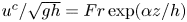 $u^c/\sqrt {gh}=Fr\exp (\alpha {z}/{h})$, where
  $Fr$ denotes the normalized surface current strength and
  $\alpha$ determines the decay rate of the vertical profile. Here
  $Fr={\pm }0.1$,
  ${\pm }0.2$ and
  ${\pm }0.3$ are considered where the positive (negative) sign indicates whether waves are propagating following (against) the currents. The maximum ratio of current velocity over wave celerity is less than 0.55, which is below the threshold for the critical layer. On the other hand, three
  $\alpha$ values of 2, 3 and 5 are used to represent weak to strong decay rate of the vertical profiles.
In figure 1, the accuracy of wave celerity is shown. The ratios of the present  $S2$ model results (
 $c_m$) and the solutions from the Rayleigh equation (
 $c_e$) are plotted for different current intensities (
 $Fr$) and magnitudes of shear (
 $\alpha$). Three panels in the figure correspond to three
  $\alpha$ values, and within each panel the upper (lower) half of the plot represents scenarios of wave propagating against (following) the current. Note that the upper half of the vertical axis is being reversed for better visualization. The red, blue and green lines indicate the magnitude of the surface current strength of
  $Fr={\pm }0.1$,
  ${\pm }0.2$ and
  ${\pm }0.3$, respectively, and the black dashed lines represent the pure wave without current scenarios.

Figure 1. Accuracy of wave celerity of linear waves riding on exponentially sheared currents with different magnitude of shears ((a)  $\alpha =2$; (b)
  $\alpha =3$; (c)
  $\alpha =5$) and different intensities (red line,
  $\lvert Fr \rvert =0.1$; blue line,
  $\lvert Fr \rvert =0.2$; green line,
  $\lvert Fr \rvert =0.3$) The upper part and lower part of each panel are the results for opposing currents and following currents, respectively. Pure wave scenarios are indicated by the dashed lines in each panel.
According to figure 1, the following general observations can be made. First, the present  $S2$ model is accurate for a wide range of
  $kh$ values up to
  $kh\approx {\rm \pi}$, approaching the deep water limit, which is characteristically the same as that of the pure wave scenario. Second, the accuracy of the wave celerity for vertically sheared currents (coloured lines) deviates from that of the pure wave scenario (dashed lines) more significantly for stronger surface currents (i.e. larger
  $\lvert Fr \rvert$ values) and stronger shears (i.e. larger
  $\alpha$ values). Third, although stronger opposing currents reduce the model accuracy (smaller applicable range of
  $kh$) for the case of
  $\alpha =2$ (figure 1a), for the case with
  $\alpha =5$ (figure 1c), the applicable range of
  $kh$ is further extended for stronger opposing currents. Vice versa for the following currents situations. Lastly, the observations for the
  $\alpha =3$ case (figure 1b) show a trend similar to the
  $\alpha =5$ case.
The above theoretical analysis shows specifically that the present models are able to produce the correct dispersion relations of small-amplitude waves on exponentially sheared currents, and have similar accuracy as that of pure wave. However, the model behaviours are affected by the vertical profile and the intensity of the current. The models using higher-order polynomial approximations are expected to produce results with similar trends.
4. Numerical solutions and discussion
The present models are implemented numerically in both 1DH and 2DH space using the same method as discussed in YL20. In the absence of currents, the models have been validated with several 3D benchmark laboratory experiments for wave propagation over uneven bottoms. These problems include (1) wave propagation over an elliptical shoal on a sloping bottom (Berkhoff, Booy & Radder Reference Berkhoff, Booy and Radder1982), (2) wave propagation over a semi-circular shoal (Whalin Reference Whalin1971), (3) solitary wave runup on a conical island (Liu et al. Reference Liu, Cho, Briggs, Kanoglu and Synolakis1995) and (4) irregular wave propagation over a submerged shoal (Vincent & Briggs Reference Vincent and Briggs1989). Comparisons show excellent agreement; they are presented in supplementary materials § A for brevity.
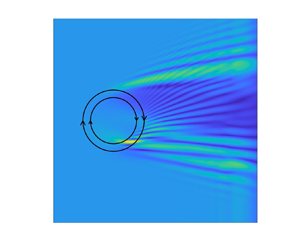
The present models are also applied to various topics on the wave–current interactions. In 1DH space, the numerical models are first validated by laboratory experiments of finite-amplitude waves propagating over uniform or linearly sheared currents (Swan Reference Swan1990). Good agreements are obtained for free surface profiles and velocity field. The details of these validations are presented in supplementary materials § B. In § 4.1.1 periodic waves of different relative water depths and nonlinearity on currents of different profiles are validated and further investigated. In § 4.1.2, solitary waves of different nonlinearity on currents of a variety of profiles are studied. By checking these 1DH problems in a constant water depth ensures the capability of present models for studying complex wave transformation problems considering sheared currents in both horizontal and vertical directions and varying bathymetry, which is the major advantage of present models over other numerical/analytical methods. These features are illustrated in 2DH investigations in § 4.2, which includes two scenarios: (1) wave propagation over a horizontal sheared vortex-ring current in constant depth (Mapp, Welch & Munday Reference Mapp, Welch and Munday1985) and (2) a wave transformation under the combined effects of a 3D sheared current and varying bathymetry.
4.1. Wave–current interactions in 1DH space
4.1.1. Finite-amplitude periodic waves on arbitrarily sheared currents
Using a 2D stream function formulation, Chen & Basu (Reference Chen and Basu2021) obtained numerical solutions for large-amplitude periodic waves on sheared currents on the vertical plane. The present model is validated with a case of nonlinear Stokes waves on currents of constant horizontal vorticity. Following Chen & Basu (Reference Chen and Basu2021), the water depth is 200 m and the target wave height and wavelength are  $H=10.08$ m and
  $L=155.91$ m, respectively. The current has a surface velocity of
  $1.31\,{\rm m}\,{\rm s}^{-1}$ and decreases to zero at the bottom. Three scenarios are considered, namely, (a) pure wave, (b) waves on following linearly sheared currents and (c) waves on opposing linearly sheared currents. To reach the same target wavelength under different current configurations, the wave period (
 $T$) is specified to be 9.79, 9.10 and 10.60 s, respectively, in Chen & Basu (Reference Chen and Basu2021). Finally, the dimensionless parameters are
  $kh\approx 8.06$ and
  $ka \approx 0.20$, which corresponds to a third-order Stokes wave in deep water.
A numerical wavemaker algorithm is employed to generate the desired waves. This algorithm was first proposed by Lee & Suh (Reference Lee and Suh1998); Lee, Cho & Yum (Reference Lee, Cho and Yum2001) and Hsiao et al. (Reference Hsiao, Lynett, Hwung and Liu2005) extended the original algorithm from a line source to a spatially distributed source. Based on the mild-slope equations, Schäffer & Sørensen (Reference Schäffer and Sørensen2006) provided the theoretical derivation of the wavemaker algorithm. A more detailed discussion on the algorithm can be found in Appendix B. The sponge layer treatment (Larsen & Dancy Reference Larsen and Dancy1983) is used at both ends of the numerical flume to absorb outgoing waves. In the numerical simulations, a horizontally uniform current with a certain vertical profile is specified by  $u^*$. A transition region is introduced to control the current effects horizontally, changing from zero in the wave generation region to full strength away from the wave generation region (Nwogu Reference Nwogu2009). To accomplish this, a ramp-up function, changing from 0 to 1, is multiplied to the terms being associated with the prescribed current (those terms are shown in Appendix A) so as to allow waves to propagate gradually from calm water into the current region with full strength.
Because of relatively large  $kh$ and
  $ka$ values, the
  $S4$ model is used to carry out all the simulations with spatial and temporal resolutions of
  $\Delta x=L/53$ and
  $\Delta t=T/80$. The numerical solutions quickly reach a quasi-steady and uniform state and figure 2 shows the comparisons of phase-averaged free surface elevations and horizontal velocity profiles under the wave crest for all three cases between the present numerical results and those of Chen & Basu (Reference Chen and Basu2021). It should be noted that the results for free surface elevation obtained from both approaches are almost the same for all three cases. Thus, only one set of results from each model is included in figure 2(a), for comparison. The present
  $S4$ model can well capture the wave free surface elevations with slight discrepancies appearing at the crest and trough. By using the wave periods specified in Chen & Basu (Reference Chen and Basu2021), the resulting waves in each scenario reach the same target wavelength, verifying the accurate frequency dispersion relation under the combined effects of third-order amplitude dispersion and wave–current interactions (Doppler-shift effects) embedded in the present model. On the other hand, the cubic function employed by the
  $S4$ model can also capture reasonably well the total horizontal velocity profiles in the entire water column as shown in figure 2(b). However, small undulations appear in the velocity profiles in the water column, and the surface velocity is underestimated slightly, whereas the bottom velocity is overestimated slightly.

Figure 2. Comparisons of (a) free surface elevation and (b) horizontal velocity profiles under the wave crest between present numerical results and those of Chen & Basu (Reference Chen and Basu2021).
Swan & James (Reference Swan and James2000) derived a second-order Stokes wave-type analytical solutions with the consideration of vertically sheared currents. Here, we check the performance of present models by comparing our solutions with those of Swan & James (Reference Swan and James2000) for a weakly nonlinear wave ( $T=10$ s,
  $h=200$ m,
  $ka=0.1$) on an exponentially sheared current of the form
  $U(z)=2\exp (0.02z)$. Note that Swan & James (Reference Swan and James2000) did not provide the explicit solutions for the free surface elevation. Therefore, in figure 3(a) only the present model's results of phase-averaged free surface elevations are shown. However, the wavelength can be compared directly between the present model results and Swan & James's (Reference Swan and James2000) analytical solutions; the difference is only less than 0.2 %. In Swan & James (Reference Swan and James2000) the wave-induced horizontal velocity was defined as the total velocity minus the prescribed current velocity. This wave-induced velocity under the wave crest is plotted in figure 3(b) and is compared with corresponding velocity
  $u'$ in the present model. Strictly speaking these two quantities are different in definition, but they should be close. The present solutions exhibit undulations because of higher degree of polynomial approximation employed in the
  $S4$ model. However, the overall agreement is quite good, especially close to the free surface where the actions are.

Figure 3. (a) Numerical results ( $S4$ model) of free surface elevations. (b) Comparisons of wave-induced horizontal velocity profiles under the wave crest between numerical results (
 $S4$ model) and Swan & James (Reference Swan and James2000).
In the previous example we have shown that the present model can perform well in the deep-water wave conditions, which is a severe test for any depth-integrated models. In the next example, the present models will be checked for their capabilities for simulating nonlinear waves in finite water depths interacting with currents with more complex profiles in the water column. We consider nonlinear periodic waves with two complex current profiles: the exponential profile,  $u^c/\sqrt {gh}=0.13\exp [6(z/h)]$, and the sinusoidal profile,
  $u^c/\sqrt {gh}=0.13\sin [{\rm \pi} (z/h+1)]$, where
  $u^c$ and
  $\sqrt {gh}$ are the current velocity and shallow-water wave celerity, respectively. The normalized current velocity profiles in the water column are shown in figure 4. A distinguishing feature between these two current profiles is the pattern of their slopes (vertical shears). Although the slope (shear) of the exponential profile is always positive in the water column with its maximum value at the still water surface, the slope (shear) of the sinusoidal current profile changes sign from negative in the upper half of the water column to positive in the lower half water column. In figure 4, the current profiles are also approximated by quadratic (dashed lines) and cubic polynomials (dash-dotted lines). Although the quadratic approximation is reasonable for the sinusoidal profile, very large discrepancies appear throughout the water column for the exponential profile, suggesting that YL20's
  $S3$ model would not be able to model these current profiles accurately, especially for the exponential current profile. Overall the cubic approximation models both current profiles more closely, but it still cannot accurately capture the correct surface, bottom and maximum velocity for these two profiles. On the other hand, the present
  $S3$ model takes the current velocity profile into consideration without further approximation and, therefore, it is a more accurate approach. Finally, the incident wave conditions are prescribed as follows: wave amplitude,
  $a=0.1$ m; wave period,
  $T=2$ s; constant water depth,
  $h=1$ m. The corresponding wavelength is
  $L_w=5.306$ m, and the dimensionless wave parameters,
  $kh=1.18$ and
  $ka=0.12$ or
  $H/h=0.2$, are obtained based on the third-order Stokes wave theory.

Figure 4. Normalized current velocity profiles. The black solid line denotes the exponential current profile  $u^c/\sqrt {gh}=0.13\exp [6(z/h)]$ and the red solid line represents the sinusoidal current profile
  $u^c/\sqrt {gh}=0.13\sin [{\rm \pi} (z/h+1)]$. The dashed lines and dash-dotted lines are the quadratic and cubic polynomial fitted results, respectively.
In total four wave–current interactions cases are considered, i.e. waves on following (opposing) exponentially (sinusoidally) sheared current, and the numerical setup is the same as previous cases in this section. The resulting free surface elevations for four wave–current interaction scenarios and the wave-alone case are shown in figure 5. Overall, the wavelength is always lengthened when waves are propagating in the same direction as the current (see figure 5d,e). The opposite is true when waves propagate against the current (see figure 5a,b). The current with a sinusoidal profile in the water column has stronger effects on waves than the current with an exponential profile does. Quantitatively speaking, when waves are propagating against (following) the current with sinusoidal profile and exponential profile, wavelengths are 12 % and 8.0 %, respectively, shorter (longer) than that of the pure wave scenario.

Figure 5. Comparisons of free surface elevations for (a) waves against current with sinusoidal profile in water column, (b) waves against current with exponential profile, (c) wave alone, (d) waves following current with exponential profile and (e) waves following current with sinusoidal profile. The horizontal axis is horizontal distance  $(x)$ normalized by the wave-alone wavelength
  $L_w$.
The exponentially sheared current has a horizontal vorticity of  $\varOmega _c=2.4\,{\rm s}^{-1}$ at the still water level. A snapshot of the calculated velocity and horizontal vorticity field for waves propagating against the exponentially sheared current (waves are propagating to the left) is shown in figure 6, where the vorticity field is normalized by
  $\varOmega _c$. As the current velocity and the wave particle velocity are in the same order of magnitude, the total velocity is almost zero at the wave crest. Moreover, the negative horizontal velocity under the wave trough is enhanced by the presence of the current. As for the vorticity field, when the wave is absent, the vorticity field is uniform in the horizontal direction, but has a maximum value at the still water surface (
 $z/h =0$) and decays into the water column. With the consideration of waves, the vertical stratification of the vorticity field is stretched or compressed as the wave comes by. This feature is further illustrated in figure 7, where the vertical profiles of the total horizontal velocity and vorticity at five phases, evenly spaced from wave crest to trough, are shown. The total horizontal velocity is normalized by the maximum horizontal velocity estimated from Stokes wave theory without current. In the same figure, the profiles of the horizontal velocity and vorticity for the pure current are also plotted. They match well with the corresponding profiles of wave–current interaction at the phase of
  $\eta =0$.

Figure 6. The velocity field (arrows) and vorticity field (colour) for waves on opposing current with an exponential profile. Waves propagate to the left and currents move to the right.

Figure 7. (a) The vertical profiles of horizontal velocity for waves on opposing current with an exponential profile. Red lines represent the total horizontal velocity at different phases from wave crest to wave trough (left to right) with equal increment; black dashed line denotes the pure current profile without waves. (b) The corresponding vertical profiles of the vorticity field. Black dashed line denotes the vorticity profile for current without waves.
Similar analyses are performed for waves on the sinusoidally sheared current. A snapshot of velocity and vorticity fields for waves propagating against the current is shown in figure 8. The horizontal velocity on the wave crest is negative (in the same direction as that of the wave propagation) and reverses its direction twice at approximately  $z/h=-0.2$ and
  $z/h=-0.8$, which is strongly influenced by the sinusoidal current profile. Figure 9 shows the vertical structure of the horizontal velocity and vorticity at different phases from wave crest to trough. The variation of the vorticity structure again follows the free surface motions, and the influence of the wave motion on the vorticity field mainly takes effect for
  $z/h>-0.8$. For brevity, the discussions on the results for waves following currents are presented in supplementary materials.

Figure 8. The velocity field (arrows) and vorticity field (colour) for waves on opposing current with a sinusoidal profile. Waves are propagating to the left and currents move to the right.

Figure 9. (a) The vertical profile of horizontal velocity for waves on opposing sinusoidally sheared current. Red lines represent the total horizontal velocity at five phases from wave crest to trough (left to right) with equal increment. Black dashed line denotes the velocity profile for current without waves. (b) The corresponding vertical profiles of vorticity for waves on opposing current with a sinusoidal profile. Black dashed line denotes the vorticity profile for current without waves.
Finally, the vertical profiles of time-averaged horizontal velocity (averaged over five wave periods) are shown in figure 10(a,b). For both exponential and sinusoidal current profiles, comparing with the prescribed current profile below wave trough, the model result is weaker when waves follow the current and is stronger when waves are against the current. Furthermore, comparing the current profiles obtained by superimposing the time-averaged velocity associated with wave-alone and the prescribed steady-state currents with the numerical model results, it can be observed that wave–current interactions (numerical model results) induce stronger (weaker) time-averaged velocities if  ${\partial u^c}/{\partial z}>0$ (
 ${\partial u^c}/{\partial z}<0$), and is independent of the wave propagation direction. Between the wave trough and wave crest, the time-averaged horizontal velocity profiles are drastically different from those obtained from the combinations of the prescribed steady-state current and the time-averaged velocity induced by wave alone. It is not surprising because the model considers the full interactions between waves and currents. Lastly, the time-averaged and depth-integrated volume flux in the water column is calculated, and the difference between numerical results of wave–current interaction and linear superimposition of those obtained from wave-alone and current-alone simulations is less than
  $2\,\%$ for all cases considered here.

Figure 10. Vertical profiles of the time-averaged horizontal velocity for waves on currents with (a) exponential profile and (b) sinusoidal profile in the water column, respectively. The black line represents the current-alone case; the black dashed line denotes the wave-alone case; the blue line shows the results of waves on following currents (numerical); the red line represents waves on opposing currents (numerical); the blue dash-dotted line denotes waves on following currents (linear superposition of wave-alone and current-alone); the red dash-dotted line represents waves on opposing currents (linear superposition of wave-alone and current-alone cases).
4.1.2. Solitary waves on arbitrarily sheared currents
In this section, the effects of arbitrarily sheared current on solitary waves are examined. As indicated in table 1 and figure 11 several current profiles are considered. The exponential velocity profile mimics the wind-induced current (Swan et al. Reference Swan, Cummins and James2001), whereas the 1/7 power profile represents a high-Reynolds-number open channel flow (Peregrine Reference Peregrine1976). The Froude number ( $Fr$) is defined as the ratio of the current velocity at the still water level (
 $u^c_s$) and the linear shallow-water wave celerity (
 $c_0=\sqrt {gh}$). The sign of the Froude number indicates whether the wave is propagating following (
 $+$) or against (
 $-$) the current. The prescribed steady-state currents are uniform in the direction of solitary wave propagation and have a maximum velocity at the still water level (
 $z =0$) and decrease to zero at the bottom (
 $z=-h$).

Figure 11. Sketch of current profiles listed in table 1 with  $Fr=1$. 1. Exponential:
  $u^c/c_0=Fr \exp (10z/h)$. 2. Cubic:
  $u^c/c_0=Fr(1+z/h)^{3}$. 3. Quadratic:
  $u^c/c_0=Fr(1+z/h)^{2}$. 4. Linear:
 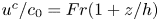 $u^c/c_0=Fr(1+z/h)$. 5. Square root:
  $u^c/c_0=Fr(1+z/h)^{1/2}$. 6. 1/3 power
  $u^c/c_0=Fr(1+z/h)^{1/3}$. 7. 1/7 power
  $u^c/c_0=Fr(1+z/h)^{1/7}$, where
  $c_0=\sqrt {gh}$.
Table 1. Test cases for solitary waves interacting with vertically sheared currents.

In the numerical simulations, the water depth is set to be  $h= 1$ m. The leading order Boussinesq solitary wave solutions (Boussinesq Reference Boussinesq1872) are employed as the initial conditions. The spatial resolution of
  $\Delta x=0.3h, 0.2h, 0.1h$ is used for solitary wave of different nonlinearity, i.e.
  $A/h=0.1, 0.2, 0.5$, respectively. The corresponding temporal resolutions are 0.1, 0.06 and 0.03 s, respectively. As the Boussinesq solitary wave solutions are not the final solutions of the present wave–current system, small trailing waves are generated at the beginning of the simulations and are left behind the leading soliton due to the differences in propagation speeds. Because of these trailing waves, the amplitude of the initial input soliton form is determined by trial and error until a solitary wave with the desired amplitude is generated (Gobbi, Kirby & Wei Reference Gobbi, Kirby and Wei2000; Lynett & Liu Reference Lynett and Liu2004). In this study, for solitary waves of
  $A/h=0.1$ and 0.2, because of the relatively small amplitude of the solitary waves and the existence of vertically sheared currents, it takes a relatively long distance of propagation (roughly 800 water depths) for the leading soliton to be separated from the trailing waves. On the other hand, a distance of only 200 water depth is necessary for the solitary wave of
  $A/h=0.5$.
The present models are first validated using the perturbation solutions of Pak & Chow (Reference Pak and Chow2009). In figure 12(a) the free surface profiles for the solitary wave of  $A/h=0.1$, following and opposing a current with linear profile (
 $|Fr|=0.6$), are compared with the third-order (in terms of
  $\epsilon =A/h$) perturbation solutions of Pak & Chow (Reference Pak and Chow2009). The free surface profile becomes narrower when the solitary wave follows the current, whereas the free surface profile is widened by the opposing current. Overall the agreement between the numerical results and the perturbation solutions is very good.

Figure 12. Comparisons of the free surface profiles of solitary waves ( $A/h=0.1$) on following and opposing currents between the present numerical results and those of Pak & Chow (Reference Pak and Chow2009). (a) Froude number
  $|Fr|=0.6$. Present model results: blue solid line, no current; red solid line, opposing linear current profile; green solid line, following linear current profile. Lines in black are the corresponding results from Pak & Chow (Reference Pak and Chow2009). (b) Froude number
  $Fr=-1.2$. Present model results: red line, opposing linear current profile (
 $S2$ model); dashed blue line, opposing square root current profile (
 $S3$ model); thick blue line, opposing square root current profile (
 $S5$ model). Numerical results from Pak & Chow (Reference Pak and Chow2009): dash-dotted black, opposing linear current profile; dotted black, opposing square root current profile.
It should be noted that the  $S2$ model is used to produce the numerical results shown in figure 12(a). However, models of higher approximations may be required when the current has different current profiles and its intensity (
 $Fr$) becomes stronger. This feature is demonstrated in figure 12(b), in which numerical results for a stronger opposing current with
  $Fr=-1.2$ with both linear current profile and square root shear profile (profile number 5 in figure 11) are plotted. For the linear current profile, the red line in figure 12(b), which is the converged results from the
  $S2$ model, agrees well with Pak & Chow (Reference Pak and Chow2009). For the square root current profile, however, the
  $S5$ model is needed to produce the converged results, which agree well with the solution from Pak & Chow (Reference Pak and Chow2009). The higher approximations make the wave profile narrower and closer to the converged results (e.g. dashed blue line which is from the
  $S3$ model). This suggests that although a model of a lower approximation can consider the exact current profile, in the case of a strong current with a complex profile, models of higher approximations may necessary to obtain the converged solutions by providing more corrections through
  $u'$.
$u'$.
The free surface profiles of finite-amplitude solitary wave with  $A/h=0.2$ and 0.5 on vertically sheared current are also studied here. Figure 13(a) shows the comparison of free surface profiles of the solitary wave (
 $A/h=0.2$) on a following current with a linear profile (
 $Fr=0.114$) between the numerical results and solutions from a weakly dispersive fully nonlinear model (Choi Reference Choi2003). The converged results from the
  $S2$ model predict a slightly narrower profile compared with the solutions from Choi (Reference Choi2003). For solitary waves with a larger amplitude of
  $A/h=0.5$, we first compare free surface profiles of the solitary wave without current obtained from the
  $S2$ model with Fenton's (Reference Fenton1972) ninth-order solution, which is shown in figure 13(b). The agreement is extremely good. In the presence of an opposing current, a solitary wave with the same amplitude is wider than that for the no current situation. The numerical results (
 $S2$ model) of the surface profile of solitary wave (
 $A/h=0.5$) on current with a linear profile and
  $Fr=-1.0$ is shown by the red line in figure 13(b), where the third-order solution from Pak & Chow (Reference Pak and Chow2009) is also included for comparison. The converged results from the present model predict a slightly wider profile than the weakly nonlinear and weakly dispersive solution. Lastly, to demonstrate the advantage of present models in taking into account arbitrarily sheared current, the free surface profile of solitary wave (
 $A/h=0.5$) on current with 1/7 power profile (no. 7 in figure 11) is considered, and the converged result from
  $S2$ model is shown by the green line in figure 13(b). Although the surface current velocity remains the same for different current profiles, the free surface profile of the solitary wave on a current with a 1/7 power profile is obviously narrower than that on a current with a linear profile, which may attribute to the weaker vertical shear near the surface for the 1/7 power current profile.

Figure 13. (a) Comparisons of the free surface profiles of solitary waves ( $A/h=0.2$) on following current with
  $Fr=0.114$ between numerical results (red line) and fully nonlinear solution from Choi (Reference Choi2003) (black dash-dotted line). (b) Comparisons of the free surface profiles of solitary waves (
 $A/h=0.5$). No current: numerical (blue line), ninth-order solution from Fenton (Reference Fenton1972) (black dashed line). Note these two lines are not distinguishable. Linearly sheared opposing current with
  $Fr=-1$: numerical (red line), third-order solution from Pak & Chow (Reference Pak and Chow2009) (black dotted line). 1/7 power sheared opposing current with
  $Fr=-1$: numerical (green line).
In addition to the linear and square root current profiles discussed above, the other current profiles sketched in figure 11 are also examined for the solitary wave of  $A/h=0.1$ on opposing current of
  $Fr=-0.6$ using the
  $S2$ model. One can anticipate the
  $S2$ model developed in YL20, which assume the horizontal velocity varies linearly in the water column, is not able to approximate the current profiles studied here, especially for those current profiles with strong local shear requires (e.g. the fifth-degree polynomial is needed to approximate profiles of no. 1 and no. 6 in figure 11). By using the linearly sheared current as the dividing case, figure 14(a) shows the solitary wave free surface profiles for the group of current profiles whose volume flux is larger than that of the linear profile. It is observed that the linear current profile produces the widest solitary free surface profile followed by the square root shear, 1/3 power shear, and the 1/7 power shear, though the differences among them are not large. The above observations seem to suggest that for this group of opposing currents changes in the solitary wave profile are more significant for currents with stronger surface shear.

Figure 14. Solitary wave free surface profiles on opposing currents ( $Fr=-0.6$) with different vertical profiles.
For the group of current profiles that have less volume flux than the linear profile current, the behaviour of the solitary wave free surface profiles shows different trends. Figure 14(b) shows that both the quadratic profile and cubic profile produce very similar results to those from the linear profile. A closer inspection shows that whereas the quadratic profile induces a slightly wider solitary wave profile than the linear profile, the cubic profile produces a slightly narrower solitary wave surface profile than the linear profile. However, the modification is much more significant for the exponential profile, which induces a narrower profile than the other non-uniform shear profiles in the same figure. Finally, among all the opposing currents of  $Fr=-0.6$ considered here, the solitary wave with
  $A/h=0.1$ has the widest free surface profile when the underlying current has a quadratic profile.
Similarly to § 4.1.1, the velocity and vorticity field of the solitary wave ( $A/h=0.1$) on opposing current with exponential profile and
  $Fr=-0.6$ are shown in figure 15, where the vorticity has been normalized by the maximum vorticity of pure current (in magnitude). A vortex is formed under the wave crest at approximately
  $z/h=-0.17$. Although the solitary wave propagates to the right, the velocity near the free surface is negative because of the presence of the strong opposing current. For the vorticity field, the strong vorticity at the still water level, associated with an exponential current profile, is lifted up to the free surface by the presence of the solitary wave.

Figure 15. The velocity field (arrows) and vorticity field (colour) for a solitary wave on opposing current with an exponential profile. Waves propagate to the right and currents move to the left.
Finally, figure 16 shows the wave celerity ( $C$) normalized by shallow-water wave speed (
 $c_0$) of solitary wave (
 $A/h=0.1$) on currents (
 $Fr=-0.6$) with different vertical profiles, which are also summarized in table 1. It is not surprising that solitary waves travel at a slower speed on opposing currents compared with the pure wave scenario. However, because of the vertical shear that decreases the current intensity from the surface to the bottom, the celerity of solitary wave on opposing current is larger than the linear superposition of pure wave celerity (
 $C/c_0\approx 1.05$) and current surface velocity (
 $u^c_s/c_0=-0.6$). The solitary wave celerity can vary significantly for currents with the same surface velocity but different vertical profiles. For example, compared with the wave-alone scenario, whereas the current with an exponential profile reduces the wave celerity by 4.65 %, the 1/7 power profile causes a dramatic decrease of 49.8 %. For the group of opposing currents considered here, the wave celerity decreases monotonically with the increasing volume flux of the opposing current. However, this does not imply that the volume flux of the current is the only parameter that determines the wave celerity. The detailed current vertical profile still matters. Thus, additional analysis is required to identify the controlling current parameters that influence certain wave properties, e.g. the influences of currents with the same volume flux but different vertical profiles on solitary waves.

Figure 16. Wave celerity of solitary wave on currents ( $Fr=-0.6$) with different vertical profiles in the water column. The horizontal axis is the volume flux of pure current
  $F$ normalized by the depth-uniform current flux
  $F_0$. The symbols from left to right correspond to current profiles 1 to 7 in figure 11.
4.2. Wave–current interactions in 2DH space
4.2.1. Wave propagation over a vortex-ring-like current
Vortex-ring-like currents can be generated by the Gulf Stream along eastern coastlines of the United States, which moves warm water from the Gulf of Mexico to the Atlantic Ocean (Mapp et al. Reference Mapp, Welch and Munday1985). The presence of this large-scale current may significantly modify incoming wave field, which are important for predicting both offshore and coastal wave climates. The effects of a vortex-ring-like current on linear shallow-water wave transformation have been studied using various numerical models, e.g. the parabolic approximation of Boussinesq model (Yoon & Liu Reference Yoon and Liu1989), the mild-slope equation model (Chen, Panchang & Demirbilek Reference Chen, Panchang and Demirbilek2005), the coupled-mode model (Belibassakis, Gerostathis & Athanassoulis Reference Belibassakis, Gerostathis and Athanassoulis2011) and the weakly nonlinear and weakly dispersive Boussinesq-type model (Zou et al. Reference Zou, Hu, Fang and Liu2013). In this section, in addition to the classic case of linear shallow-water incident waves, the present models are also used to examine weakly nonlinear intermediate-water-depth waves propagating over a vortex-ring-like current field, which is more realistic to the physical background of the vortex-ring-like current field. Differences in the resulting wave fields are discussed.
Following Mapp et al. (Reference Mapp, Welch and Munday1985), the depth-uniform current field ( $U_r$,
  $U_\theta$,
  $U_z$) is expressed in the cylindrical coordinates (
 $r$,
$r$,  $\theta$,
  $z$) as
 \begin{gather} U_r=0, \end{gather}
 \begin{gather}U_\theta=\left\{ \begin{array}{@{}ll} C_5\left(\dfrac{r}{R_1}\right)^N, & r \leq R_1, \\ C_6 \exp{\left[-\left(\dfrac{R_2-r}{R_3}\right)^2\right]}, & r >R_1,\end{array} \right. \end{gather}
 \begin{gather}U_z=0, \end{gather}
 \begin{gather}\eta^c={-}\frac{1}{g}\int_r^\infty\frac{U^2_\theta}{r} \,\mathrm{d}r, \end{gather}
where  $\eta ^c$ is the free surface set-down associated with the current field, which satisfies exactly the steady-state Euler equation. In (4.2),
  $R_3$ estimates the length scale of the current field and
  $C_6$ represents the maximum magnitude of current velocity. Adopting the parameters presented in previous studies (Yoon & Liu Reference Yoon and Liu1989; Zou et al. Reference Zou, Hu, Fang and Liu2013), the following values are used in the present numerical calculations,
  $N=2$,
  $R_1=343.706$ m,
  $R_2=384.881$ m,
  $R_3=126.830$ m,
  $C_5=0.9\,{\rm m}\,{\rm s}^{-1}$ and
  $C_6=1.0\,{\rm m}\,{\rm s}^{-1}$. The shapes of
  $U_\theta (r)$ and
  $\eta ^c (r)$ are shown in figure 17, in which the maximum value of
  $U_\theta$ is located at
  $R_2 =384.881$ m as denoted by a red dot.


Two kinds of incident wave conditions are considered herein. The incident wave in the first case has an amplitude of  $a_1=0.05$ m and a period of
  $T_1=19.43$ s, with
  $a_2=0.5$ m and
  $T_2=7.3$ s for the second case. The still water depth is fixed at
  $h=10$ m, yielding the following dimensionless parameters characterizing these two incident wave conditions: (
 $k_1h=0.33$,
  $k_1a_1=0.0017$) and (
 $k_2h=1.0$,
  $k_2a_2=0.05$). Thus, the first case represents a linear shallow-water wave and the second case is a second-order Stokes wave in intermediate water depth. The relative current strength (
 $C_6/\sqrt {gh}$) is fixed at 0.1. Accordingly, the wave ray patterns can be calculated from the linear wave ray theory (Arthur Reference Arthur1950; Kenyon Reference Kenyon1971) as shown in figure 18(a) for both the shallow-water wave (red lines) and the intermediate-water wave (blue lines) scenarios. In the figure, the vortex-ring-like current field, circulating in the clockwise direction, is symbolically represented by two concentric circles. The centre of the current field is located at
  $(x_0, y_0)=(1.0,0.0)$ km. The two concentric circles have a radius of
  $R_2$ and
  $R_3$, which correspond to the maximum current velocity of
  $C_6$ and the velocity of
  $C_6/e$, respectively. Without the current field, wave rays are straight lines parallel to the
  $x$-axis. In the presence of the current field, wave rays are refracted and wave ray crossings occur in a complex manner, suggesting that the linear wave ray theory is no longer valid and the wave diffraction needs to be considered.

Figure 18. (a) The wave ray patterns over a vortex-ring-like current. Red lines are wave rays for shallow-water wave ( $k_1h=0.33$); blue lines are for intermediate-water-depth wave (
 $k_2h=1.0$). (b) Contour plots of instantaneous free surface elevations at
  $t=28T_1$ for the shallow-water incident wave case.
As  $kh$ values are relatively small, the present
  $S2$ model is used to simulate both scenarios. The lengths of numerical simulations are
  $28T_1$ for shallow-water-depth and
  $75T_2$ for intermediate-water-depth cases, respectively. The spatial and temporal resolutions are
  $\Delta x=\Delta y=L/18$ and
  $\Delta t=T/20$ for both cases, where
  $T$ and
  $L$ are the period and wavelength of the incident waves, respectively. Sponge layers are applied downstream for absorbing outgoing waves. The length of the computational domain in the
  $y$-direction is set to be sufficiently long enough to guarantee that the wall boundary conditions implemented at north and south boundaries do not influence solutions in the area of interest.
In figure 18(b), the contour lines of instantaneous free surface elevations at the end of the numerical simulation ( $t=28T_1$) for the shallow-water incident wave scenario are plotted. The parallel contour lines of incident plane waves are significantly distorted by the presence of the vortex-ring-like current through wave refraction and diffraction. Referring to the wave ray patterns shown in the left panel, many surface undulations along the crest lines can be identified with the wave ray crossings.
In figure 19, spatial distributions of normalized wave heights for the shallow-water-depth ( $k_1h=0.33$) case and the intermediate-water-depth (
 $k_2h=1.0$) case are displayed. Here, the wave heights are calculated by performing the wave-by-wave zero-crossing analysis on the last five simulated waves. Note that the wavelength of the waves in intermediate water depth is one-third of that of the shallow-water wave and the incident wave amplitude of the intermediate-water-depth case is 10 times larger than that of the shallow-water wave, resulting in stronger nonlinearity for the intermediate-water-depth case. Thus, the amplification of wave height by opposing current is more obvious in the intermediate-water-depth case; the maximum wave height is located at
  $(x,y)=(1.3\,{\rm km},\ 0.4\,{\rm km})$, which is behind the maximum opposing current (the inner circle). Moreover, the vortex-ring-like current has stronger refraction effects on shorter waves, resulting in different wave patterns for these two cases, especially on the lee side of the current.

Figure 19. (a) Spatial distribution of the normalized wave heights for the case of shallow-water-depth wave ( $k_1h=0.33$). (b) Spatial distribution of the normalized wave heights for the case of intermediate-water-depth wave (
 $k_2h=1.0$).
The normalized wave heights along six transects ( $x=$ constants) for the case of shallow-water incident wave (
 $k_1h=0.33$) are shown in the left panels of figure 20. The results from a Boussinesq-type model (Zou et al. Reference Zou, Hu, Fang and Liu2013) are also shown (in black dots) in the same panel. Generally speaking, two models have produced similar results with slight discrepancies in the region of
  $y>0$, where waves follow the currents. Lastly, the wave height variations along the same transects for the case of intermediate water depth (
 $k_2h=1.0$) are also shown in the right panels of figure 20. At
  $x=1.2594$ km the maximum wave height is almost three times the incident wave height because of the enhanced nonlinearity. On the other hand, the diffracted waves behind the vortex-ring-like current show much stronger spatial variations for their shorter wavelengths.

Figure 20. Normalized wave heights along six transects ( $x=$ constants). Here
  $H_0$ is the incident wave height. (a,c,e,g) Comparisons between the present
  $S2$ model (red lines) and the Boussinesq model (Zou et al. Reference Zou, Hu, Fang and Liu2013) (black dots) for the shallow-water-depth case (
 $k_1h=0.33$). (b,d,f,h) The present
  $S2$ model results for the intermediate-water-depth case (
 $k_2h=1.0$).
For both cases, the steady current velocities from the present model are obtained by time-averaging the total horizontal velocities over the last five wave periods in the numerical simulations. The comparisons between the model results and the prescribed vortex-ring-like current (4.1)–(4.4) are made at several locations under the wave trough, showing almost identical results. For completeness, the comparisons for the intermediate-wave case are shown in the supplementary materials. The time-averaged velocities between the wave trough and wave crest can also be calculated from the present model solutions, which show very different patterns from the prescribed currents. To demonstrate this feature, in figure 21 the present model results for the time-averaged velocity at the elevation of  $z/h=-0.02$ are compared with the prescribed current velocity along four transects
  $y = 0.4$ km, 0.3 km,
  $-0.3$ km and
  $-0.4$ km. The elevation
  $z/h=-0.02$ is above the wave trough but under the current-induced mean free surfaces. The time-averaged resulting velocities are generally weaker than the prescribed current because of the periodically fluctuating free surfaces induced by waves.

Figure 21. Comparisons between the time-averaged resulting current field (red line) and the prescribed current field (black line) at four transects for  $x$ component velocity,
  $u$ (a,c,e,g) and
  $y$ component velocity,
  $v$ (b,d,f,h) at
  $z/h=-0.02$.
4.2.2. Obliquely incident wave propagation over a 3D sheared current
Whereas the examples discussed in the previous sections all have a constant depth, in this section, the present models are employed to simulate wave propagation and transformation over a varying bathymetry and a current field that shears both horizontally and vertically.
The plan view of the numerical setup is sketched in figure 22(a). A numerical wavemaker is placed at  $x=0$, generating obliquely incident waves with an incident angle of
  $15^\circ$ with respect to the
  $x$-axis, an amplitude of 0.016 m and a period of 1.2 s in a still water depth of
  $d= 0.35$ m. The corresponding dimensionless wave parameters are
  $kd=1.18$ and
  $ka=0.054$. A submerged ridge parallel to
  $y$-axis is installed inside the computational domain. The submerged ridge has the same fore-slope and back-slope of
  $1:20$ and the water depth on the crest of the ridge is 0.1 m with the corresponding ridge crest width of 1.5 m (see figure 22c). Sponge layers of 2.5 m wide are implemented on the western and eastern (
 $x$-direction) sides of the computational domain for absorbing outgoing waves, whereas wider sponge layers (8 m) are used on the northern and southern (
 $y$-direction) sides. Finally, the length of the computational domain in the
  $y$-direction is set to be
  $60$ m, which is verified to be sufficiently long to minimize influences from the sponge-layer boundaries to the central area of interest.

Figure 22. (a) The plane view of the computational domain, where the dashed areas are the sponge layers, the thick black line is the location of the wavemaker and the coloured contours indicate the current region. (b) Vertical profiles of depth-uniform current (blue line) and vertically sheared current (red line) on a flat bottom of still water depth. (c) Bottom bathymetry in the  $x$-direction.
A prescribed steady-state current field is installed inside the computational domain. The current field is unidirectional in the  $y$-direction and has a Gaussian distribution in the
  $x$-direction, which is similar to the ‘steady shear current’ pattern proposed by Smith (Reference Smith2006). However, the present current field can have different velocity profiles in the water column. The current velocity components and the free surface elevation can be expressed as follows
 \begin{gather} u^c = 0, \quad w^c = 0, \quad \eta^c = 0, \end{gather}
 \begin{gather}v^c = v^c_s g(z)=Fr\sqrt{gd} \exp{[-((x-x_0)/r)^2]}g(z), \quad -h(x)\leq z \leq 0, \end{gather}
where  $v^c_s$ is the
  $y$-component of the surface current velocity, and it has a Gaussian shape in the
  $x$-direction, being centred at
  $x_0=10$ m, which is aligned with the centre line of the ridge and has a length scale of
  $r=2$ m. The location of the current field is indicated by the contour lines in figure 22(a). The maximum intensity of the current is determined by the Froude number (
 $Fr$) and the velocity profile in the water column is defined by
  $g(z)$, where
  $-h \leq z \leq 0$. The current flows in the positive
  $y$-direction. Note that the prescribed current field over the submerged ridge satisfies the steady-state Euler equations.
In the present simulations,  $Fr=0.25$ is used so that the current is in a weak current regime with a length scale comparable to the incident wavelength, which is essentially not slowing varying. Three different scenarios are investigated: (1) pure wave propagation (no current); (2) waves on depth-uniform currents (
 $g(z)=1$); and (3) waves on vertically sheared currents with
  $[g(z)=1.1(z/h)^2+2.1(z/h)+1, -h\leq z\leq 0]$. The vertical profile of the sheared current on a flat bottom is shown by the red line in figure 22(b). Note that the current profile in the water column does not change in the
  $y$-direction. However, the profile changes at different
  $x$-cross-section because the water depth changes.
Numerical simulations are conducted using the  $S2$ model with spatial and temporal resolutions of
  $\Delta x=0.04$ m,
  $\Delta y=0.2$ m and
  $\Delta t=0.02$ s, and they are carried out for 25 wave periods, which is sufficiently long for reaching a quasi-steady state. Figure 23(a,b) show the snapshots of normalized (by incident wave amplitude) instantaneous free surface elevations for the pure wave case and depth-uniform current case in the area of interest (
 $4\,{\rm m} < x< 14\,{\rm m}$,
  $-6\,{\rm m}< y< 6\,{\rm m}$) at the end of the simulation, respectively. In figure 23(a), evidently, a train of uniform obliquely incident waves has been generated before the toe of the submerged ridge (
 $x=4.25$ m). Waves are refracted by the submerged ridge and shorter waves with larger wave amplitudes can be observed on the front face and on top of the ridge (around
  $x= 10$ m) because of shoaling effects. Compared with the pure wave case, the wavelengths for the depth-uniform current case are longer, which can be observed in figure 23(b). The differences of instantaneous free surface elevations between the pure wave case and the uniform current case at the same instant are also shown in figure 23(c). The differences mainly appear in the region
  $x>8.5$ m, which is primarily caused by the higher wave celerity in the case of wave–current interactions.

Figure 23. The normalized instantaneous free surface elevations at the end of the numerical simulation for (a) the pure wave case and (b) depth-uniform current case, and (c) their differences.
As both waves and currents are uniform in  $y$-direction, we focus our analysis only on the transect along
  $y=0$ m. The spatial variation of the prescribed depth-uniform current and vertically sheared current velocity at two water depths (
 $z=-0.01$ m and
  $z=-0.05$ m) are shown in figure 24(a,b) by lines in black, respectively. In the same figure, the corresponding numerical results from the present models are also shown for comparison. The numerical results are obtained by time-averaging the horizontal velocities of the last five waves in the numerical simulation (at the same transect and vertical elevation). For the case of uniform velocity profile, the differences between the prescribed current velocity and the model results are only noticeable at the water depth of
  $z=-0.01$ m, and the wave effects on the current field below the wave trough are very small. For the vertically sheared current case, whereas there is a significant difference at the water depth of
  $z= -0.01$ m, small differences can also be observed for
  $z= -0.05$ m, which may be attributed to the relatively abrupt changes of the bottom.

Figure 24. (a) The spatial variation of the time-averaged velocities along  $y=0$ m at
  $z=-0.01$ m (blue dash-dotted line) and
  $z=-0.05$ m (blue line) for uniform current case. The prescribed current at these two water depths are shown by lines in black. (b) The spatial variation of the time-averaged velocities along
  $y=0$ m at
  $z=-0.01$ m (red dash-dotted line) and
  $z=-0.05$ m (red line) for vertically sheared current case. The prescribed current at these two water depths are shown by lines in black. (c) The snapshot of free surface elevations at the end of simulations for pure wave (black), waves on depth-uniform current (blue), and waves on vertically sheared current (red) at
  $y=0$ m. (d) The spatial variation of wave heights for pure wave (black), waves on depth-uniform current (blue), and waves on vertically sheared current (red) at
  $y=0$ m. Here
  $\eta _0$ and
  $H_0$ are the incident wave amplitude and height, respectively.
Snapshots of the normalized instantaneous free surface elevations for all three cases are also shown in figure 24(c). The differences of free surface elevations in these three cases become significant starting from  $x> 9.0$ m, which are caused by the combined effects of bathymetric variation and sheared currents. Both current fields make wave celerity faster and the depth-uniform current has more significant effects. Waves also become higher and higher harmonic waves are generated by shoaling effects, which can be clearly seen on top of the ridge. Wave heights are also calculated from the last five waves of each simulation and their spatial distributions are plotted in figure 24(d). On the front slope of the ridge, the shoaling effects tend to amplify the wave height, the following current act in an opposite way, which reduces the wave height. Compared with wave-alone scenario, the wave heights on the front slope of the ridge can be
  $5.5\,\%$ and
  $2.1\,\%$ smaller for depth-uniform current and vertically sheared current, respectively. On top of the ridge, the wave heights for the vertical sheared current case is even larger than the wave-alone scenario, followed by the depth-uniform current case. However, the effects of the vertical shear is less obvious on the back-slope of the ridge, where the current magnitude decreases, and the wave heights of wave–current interaction cases are approximately 5–
 $10\,\%$ larger than that of wave-alone situation. It is also interesting to note that the nonlinear features at downstream are also more significant for cases with currents, which can be observed from both figures 24(c) and 24(d).
5. Concluding remarks
This paper offers further extension and improvement of the depth-integrated wave–current models developed in YL20. The new models are now capable of incorporating exactly the arbitrarily sheared current profile in the formulation. The applications have also been extended from 1DH problems to 2DH examples.
A theoretical linear Stoke wave-type analysis has been conducted on the  $S2$ model to find the embedded frequency dispersion relation for a linear wave riding on currents with an exponential profile. The results have been compared with the corresponding theoretical estimations based on the Rayleigh equation. The influence from the direction, intensity and vertical structure of the current field on the applicable range of
  $kh$ values of the present models has been investigated. It has been found that the present models are capable of capturing the correct dispersion relation comparable to that of pure wave scenarios. However, the accuracy of the model may deteriorate for currents with strong intensity and vertical shear close to the free surface.
The critical layer could occur near the free surface when shorter waves interacting with wind-induced sheared currents, where more detailed discussions can be found in Maslowe (Reference Maslowe1986), Craik (Reference Craik1988) and Drazin & Reid (Reference Drazin and Reid2004). A full analysis of critical layers should consider viscous effect. However, in terms of the stability of the Rayleigh equations the inviscid treatment is nevertheless informative (Ellingsen & Li Reference Ellingsen and Li2017). In the present studies, the current velocity is always less than the wave celerity for all the periodic wave cases, which is below the threshold for the critical layer. However, further analysis on the critical layer using present models would be of interest.
Without considering the current effect, the present models have been validated by several 3D benchmark laboratory experiments, in which the wave refraction, diffraction and runup induced by bathymetry have featured. These results are documented in the supplementary materials.
Various wave–current interaction problems have then been studied in 1DH space. For periodic waves, the present models have been validated by analytical and numerical results for nonlinear deep-water waves on vertically sheared currents. Numerical experiments have then been conducted to examine the effects of more complicated current profiles, i.e. exponential and sinusoidal profiles, on finite-amplitude periodic waves in intermediate water depth. It has been found that the wave–current interaction for a positively (negatively) sheared current, i.e.  ${\partial u^c}/{\partial z}>0$ (
 ${\partial u^c}/{\partial z}<0$), results in stronger (weaker) time-averaged velocity than that of the superposition of time-averaged velocity associated with the wave-alone and the prescribed current, which is also independent of the wave propagation direction.
The interaction between a finite-amplitude solitary wave and currents with various vertical profiles has also been examined. The resulting solitary wave free surface elevations, wave celerity, velocity and vorticity fields have been discussed. For the group of currents considered here, which share the same surface velocity but different vertical profiles, the wave celerity decreases monotonically as the volume flux of the opposing current increases. However, this does not imply that the volume flux of the current is the only parameter that determines the wave celerity. The detailed current vertical profile, especially close to the free surface, still matters. Lastly, it has been found that the solitary wave free surface elevations cannot be straightforwardly related to the volume flux of the current, i.e. a monotonic trend has not been found between the width of the solitary wave and the volume flux of the current.
For periodic waves interacting with vertically sheared currents, we have shown the time-averaged velocity profiles up to the wave crest in the water column, which are converged results by checking models of different approximations. Specifically, the time-averaged velocities between the wave trough and crest demonstrate that the prescribed steady current field is significantly influenced by surface wave motions, which is drastically different from the linear superimposition of time-averaged velocity induced by the wave-alone and prescribed current. However, the time-averaged volume flux across the entire water column remains the same.
Two examples for simulating wave–current interactions in 2DH space have been given. The scattering of shallow-water waves and intermediate-water waves by a vortex-ring-like current field has been investigated. We have found that the diverging and converging phenomena are more significant for the intermediate-water waves than the shallow-water waves because of much shorter length scales compared with currents. The combined effects of a 3D sheared current field and varying bathymetry have further been demonstrated by conducting numerical experiments for oblique incident waves propagating into an infinite long submerged ridge and a both vertically and horizontally sheared current field, whose direction is aligned with the submerged ridge. Various physical processes, including higher harmonic generation due to the sloping bottom, and waves interacting with currents of horizontal and vertical shears, have been identified. Specifically, it has been observed that the current with vertical shear results in quite different wave celerity and wave height distributions compared with the depth-uniform current. This implies that it is important to model the current field accurately, including its vertical profile, before considering wave–current interaction problems. Finally, for both cases the time-averaged velocity fields have been obtained, whereas obvious differences have been found compared with the prescribed current field at the elevation between the crest and trough, the current field under the wave trough seems to show small variations compared with the prescribed current.
The models developed in this paper offer a new approach for studying waves interacting with a prescribed steady-state current field which may have complex vertical profiles in the water column. Compared with YL20, the present models are more advantageous when waves are in a relatively shallow depth, which requires lower polynomial approximations, interacting with currents of complex vertical structures. Considering the present numerical models are capable of employing any degree of polynomial approximations together with arbitrary current distributions, they are expected to simulate a wide range of wave–current interactions problems from deep water to shallow water together with various current configurations in the future.
The present formulations are still based on the Euler equations. In the future, other physical processes such as viscous and turbulent effects will be introduced to offer a more comprehensive description of the wave–current interaction problems, especially the contribution from these mechanisms on the modifications of the current field under wave–current interactions.
Supplementary material
Supplementary material is available at https://doi.org/10.1017/jfm.2022.42.
Funding
P.L.-F.L. would like to acknowledge support from the National University of Singapore, Cornell University and the National Research Foundation in Singapore through a research grant (NRF2018NRF-NSFC003ES-002). Z.T.Y. would like to thank the Ministry of Education in Singapore for a Ph.D. Scholarship. The work presented in this paper is a result of the research effort through Enhancing Offshore System Productivity, Integrity and Survivability in Extreme Environments (ENSURE) programme supported by A*STAR under its RIE 2020 Industry Alignment Fund (Grant No. A19F1a0104).
Declaration of interests
The authors report no conflict of interest.
Author contributions
Z.T. Yang: conceptualization; model formulation; analytical analysis; numerical simulations; writing. P.L.-F. Liu: conceptualization; writing - review and editing; supervision; project administration.
Appendix A. Depth-integrated horizontal momentum equations
In this section, the resulting depth-integrated horizontal momentum equation (2.24) is shown in details. We recall that if  $u^*_i$, which is responsible for the prescribed current field, can be expressed as follows:
 \begin{equation} u_i^*(x_i,\sigma)=f(x_i)g_i(\sigma), \end{equation}
then the corresponding vertical velocity component is
 \begin{equation} w^*_i={-}G_i(\sigma)\frac{\partial H}{\partial x_i}+u^*_i\left(-\frac{\partial h}{\partial x_i}+\sigma\frac{\partial H}{\partial x_i}\right), \end{equation}
where
 \begin{equation} G_i(\sigma)=\int_0^\sigma g_i(\sigma) \,\mathrm{d}\sigma. \end{equation}
 Depending on the vertical dependence of each term, the  $H_{mtm}$ term in (2.24) can be organized into the following form
 \begin{align} H_{mtm}&=\underbrace{\sum_{m=1}^KH^{w}_{m}\sigma^{m-1}+\sum_{m=1}^K\sum_{n=1}^KH^{w}_{m,n}\sigma^{m+n-1}}_\text{terms in YL20}\nonumber\\ &\quad +\sum_{m=1}^K\left(H^{wc1}_m\sigma^{m-1}g_i+H^{wc2}_m\sigma^{m}g_i'+H^{wc3}_m\sigma^{m-2}G_i\right)\nonumber\\ &\quad +\sum_{m=1}^K\left(H^{c1}_mG_ig_i'+H^{c2}_mg_i^2+H^{c3}_m\sigma g_i'\right), \end{align}
where  $g_i'$ is the first derivative of
  $g_i(\sigma )$, and
  $H^{w}_{m}$,
  $H^{w}_{m,n}$,
  $H^{wc1}_m$,
  $H^{wc2}_m$,
  $H^{wc3}_m$,
  $H^{c1}_m$,
  $H^{c2}_m$ and
  $H^{c3}_m$ are only functions of horizontal coordinates and time. For brevity, they are given in the supplementary materials. We remark that models developed in YL20 only contain terms in the first line of (A4).
Similarly,  $V_{mtm}$ in (2.24) can be organized as
 \begin{align} V_{mtm}&=\underbrace{\sum_{m=1}^K(V^{w1}_{m}\sigma^{m-1}+V^{w2}_{m}\sigma^{m})+\sum_{m=1}^K\sum_{n=1}^K(V^{w1}_{m,n}\sigma^{m+n-2}+V^{w2}_{m,n}\sigma^{m+n-1})}_\text{terms in YL20}\nonumber\\ &\quad +\sum_{m=1}^K(V^{wc1}_{m}\sigma^{m-1}g_i+V^{wc2}_{m}\sigma^{m}g_i+V^{wc3}_{m}\sigma^{m}g'_i\nonumber\\ &\quad +V^{wc4}_{m}\sigma^{m+1}g'_i+V^{wc5}_{m}\sigma^{m-2}G_i+V^{wc6}_{m}\sigma^{m-1}G_i)\nonumber\\ &\quad +\sum_{m=1}^K(V^{c1}_{m}\sigma g_i+V^{c2}_{m}G_i g_i+V^{c3}_{m}g^2_i+V^{c4}_{m}G(\sigma) g'_i\nonumber\\ &\quad +V^{c5}_{m}\sigma g^2_i+V^{c6}_{m}\sigma g'_i+V^{c7}_{m}G_i+V^{c8}_{m}\sigma^2 g'_i+V^{c9}_{m}\sigma G_i g'_i), \end{align}
where  $V^{w1}_{m}$,
  $V^{w2}_{m}$,
  $V^{w1}_{m,n}$,
  $V^{w2}_{m,n}$,
  $V^{wc1}_{m}$,
  $V^{wc2}_{m}$,
  $V^{wc3}_{m}$,
  $V^{wc4}_{m}$,
  $V^{wc5}_{m}$,
  $V^{wc6}_{m}$,
  $V^{c1}_{m}$,
  $V^{c2}_{m}$,
  $V^{c3}_{m}$,
  $V^{c4}_{m}$,
  $V^{c5}_{m}$,
  $V^{c6}_{m}$,
  $V^{c7}_{m}$,
  $V^{c8}_{m}$ and
  $V^{c9}_{m}$ are only functions of horizontal coordinates and time and are given in the supplementary materials. We remark that models developed in YL20 only contain terms in the first line of (A5).
The vertical and horizontal dependencies are separated by the arrangements as shown above. The vertical dependence is further removed by the vertical integration as defined in (2.24). For example, for the YL20 terms in  $H_{mtm}$ and
  $V_{mtm}$, there are only two kinds of vertical integrals involved, i.e.
 \begin{equation} A^q_p=\int_{c_{q}}^{c_{q+1}}\sigma^{p-1}, \quad B^q_p=\int_{c_{q}}^{c_{q+1}}\int_{\sigma}^{1}\sigma^{p-1}, \end{equation}
where  $q=0,1,2,\ldots, (K-1)$ and
  $p=1,2,\ldots, (2K-1)$. The above two integrals can be calculated analytically and pre-stored for later use. Other vertical integrals that are related with the prescribed steady current field can be treated in a similar way. However, for those integrals that may be difficult to integrate analytically, they can be calculated through numerical integration (e.g. trapezoidal rule). Finally, the resulting numerical model is more general and applicable to model waves on currents in the form of (A1) using any degree of approximations on
  $u_i'$.
Appendix B. Comments on the internal numerical wavemaker
In this section, the performance of the internal numerical wavemaker is discussed in detail. The generated waves will be compared with Stokes wave theory in terms of both free surface elevations and velocity field. Specifically, the observations of time-averaged mean free surface and time-averaged mean velocity are also reported.
The internal wavemaker approach used in this paper was first proposed by Lee & Suh (Reference Lee and Suh1998) and Lee et al. (Reference Lee, Cho and Yum2001). Later, Hsiao et al. (Reference Hsiao, Lynett, Hwung and Liu2005) extended the original line source to the spatially distributed source, which is that employed herein. Based on mild-slope equations, Schäffer & Sørensen (Reference Schäffer and Sørensen2006) provided the theoretical foundation of this internal wavemaker formulation. Here, we illustrate the application of the internal wavemaker for the 1DH case. The basic approach of the internal wavemaker is to add a prescribed amount of free surface elevation,  $\eta ^*(x,t)$, to the calculated surface elevation at each time step of the computation. In the present numerical models,
  $\eta ^*(x,t)$ is a simple harmonic function in time with wave period,
  $T$, and is distributed spatially as a Gaussian-shaped function. Thus, the corresponding
  $\eta ^*$ is expressed as (Hsiao et al. Reference Hsiao, Lynett, Hwung and Liu2005)
 \begin{equation} \eta^*(x^\prime,t)=\frac{\Delta t}{T}\frac{C_g}{C}\eta^I R(\beta)\exp[{-\beta(x'/L)^2}], \end{equation}
where
 \begin{gather} \eta^I= a \cos (2{\rm \pi} t/T), \end{gather}
 \begin{gather}R(\beta)=2\left[\sqrt{\frac{\rm \pi}{\beta}}\exp{\left(-\frac{{\rm \pi}^2}{\beta}\right)}\right]^{{-}1}, \end{gather}
and  $\Delta t$ is the numerical time step,
  $a$,
$a$,  $L$,
$L$,  $C_g$ and
  $C$ are the amplitude, wavelength, wave group speed and wave celerity, respectively, based on the linear wave theory and
  $x'$ is the distance to the centre of the numerical wavemaker. The effective width of the wavemaker is determined by
  $\beta$ (see Wei, Kirby & Sinha (Reference Wei, Kirby and Sinha1999) for detail) and it is taken to be
  $\beta =20$ in simulations presented in this paper, which makes the effective length to be one wavelength (Hsiao et al. Reference Hsiao, Lynett, Hwung and Liu2005). Finally,
  $R(\beta )$ is an additional coefficient induced by the spatially distributed Gaussian-shape function.
To demonstrate the effectiveness of the internal wavemaker, the wave condition of case 1 in § B of the supplementary materials is considered here: wave amplitude  $a=0.035$ m, wave period
  $T=1.412$ s and water depth
  $h=0.35$ m. This wave condition corresponds to a Stokes third-order wave in intermediate water depth with wavelength
  $L=2.33$ m,
  $kh=1.0$ and
  $ka=0.1$. Numerical simulations are performed in a 1DH domain of
  $35L$ in length. The internal source is centred at
  $x=3.9L$ and sponge layers of
  $2L$ are placed at both ends to absorb outgoing waves. The spatial and temporal resolution of
  $\Delta x=L/48$ and
  $\Delta t=T/60$ are used in the numerical experiments. Although the single harmonic wave is specified as an input in the wavemaker theory, the generated waves quickly show nonlinear features outside the generation region. Finally, the numerical simulation is terminated when waves in the computational domain reach quasi-steady-state, which takes approximately
  $35T$.
Numerical simulations are conducted using both the  $S2$ and
  $S3$ models. Once the numerical simulation ends, the zero-crossing analysis is conducted on 10 waves in the centre of the numerical flume which are away from the wavemaker and downstream boundary. The calculated wavelength is 2.32 m for both models, which is very close to the anticipated value of 2.33 m, based on the third-order amplitude dispersion relation. Phase- and time-averaging are performed on the time series of free surface elevations and horizontal velocities for the 10 waves recorded at
  $x = 16L$, close to the centre of the numerical flume, to minimize the influences from the numerical wavemaker and downstream boundary. The comparisons of the free surface elevations and horizontal velocities at three different elevations (
 $z=-0.1$ m,
  $-0.2$ m,
  $-0.3$ m) are shown in figure 25, in which the horizontal velocity is normalized by the maximum horizontal velocity predicted by the third-order Stokes wave theory. Good agreements are observed between the numerical results (of
  $S2$ and
  $S3$ models) and the theory for both free surface elevations and horizontal velocities. However, a close inspection of the vertical profiles of the horizontal velocity under wave crest and trough, as depicted in the left panel of figure 26, reveals that the
  $S2$ model provides a better agreement under the wave crest than beneath the wave trough. The vertical profile of the time-averaged horizontal velocity in the water column is also shown by the black line in figure 26. Below the wave trough, the time-averaged velocities are slightly negative, whereas the time-averaged velocities between the wave crest and wave trough are positive, namely in the direction of wave propagation. Below the wave trough (
 $-1< z/h<-0.143$), the depth-averaged mean current value is
  $-0.82\times 10^{-2}\,{\rm m}\,{\rm s}^{-1}$, which is
  $3.8\,\%$ of the maximum horizontal velocity. The time-averaged mean free surface is
  $-8.9\times 10^{-4}$ m, which is
  $2.5\,\%$ of the wave amplitude.

Figure 25. Comparisons of phase-averaged time series free surface elevations and horizontal velocities at three elevations between the numerical results (blue lines in panel (a,c,e,g),  $S2$ model results; blue lines in panel (b,d,f,h),
  $S3$ model results) and Stoke third-order theory (red lines in panels a–h).

Figure 26. Comparisons of vertical profiles of the phased-averaged horizontal velocity under the wave crest and trough between numerical results (blue lines in panel (a),  $S2$ model results; blue lines in panel (b),
  $S3$ model results) and third-order Stoke theory (red lines in panels a,b). Black lines show vertical profiles of time-averaged horizontal velocity obtained from numerical results.
The numerical results of the  $S3$ model are closer to the theory (see the right panels in figures 25 and 26), which is not surprising. The quadratic velocity profile in the water column used in the
  $S3$ model captures the theoretical profiles of the horizontal velocity beneath the wave crest more accurately. However, the velocity magnitudes under the wave trough are still larger than the theoretical solutions. It is interesting to observe that the mean free surface (
 $-8.8\times 10^{-4}$ m) and the depth-averaged mean horizontal velocity (
 $-0.84\times 10^{-2}\,{\rm m}\,{\rm s}^{-1}$) are almost the same as those obtained by the
  $S2$ model.
Numerical simulations of pure wave propagation have been conducted for other periodic wave conditions that have been discussed in this paper. Similar findings on the free surface elevations and horizontal velocity fields are also observed in all cases. Table 2 summarizes the resulting relative mean free surface and relative negative mean velocity for these wave conditions. We find the relative mean free surface is always smaller than the relative negative mean velocity. For waves with the same relative water depth, larger nonlinearity will induce larger relative mean values. This phenomenon is less obvious for deep-water waves.
Table 2. Summary of all the test cases on pure wave propagation using the internal wavemaker with  $H$ being the wave height here. The last two columns show the relative magnitude of mean free surface and mean negative velocity, respectively. Cases 1–3 correspond to test cases 1–3 in § B of the supplementary material and cases 4 and 5 are the wave conditions used in § 4.1.1.

The numerical experiments suggest that the internal wavemaker may generate a small mean free surface ‘set-down’ and a small negative mean ‘current’. This is because the input waves from the internal wavemaker do not satisfy the model equations, resulting in these mean quantities. One could try to adjust the input parameters in the internal wavemaker so as to eliminate these mean quantities. However, it is a non-trivial exercise due to the complex nonlinear properties in the models and the smallness of the mean quantities. Although we do not expect that these mean quantities will alter the pure wave propagation and wave–current interaction processes because of their small magnitude, however, the need for improving the implementation of the boundary conditions associated with the incident wave properties or a better numerical wavemaker algorithm should be noted.


 Open access