


1. Introduction
Evaporating droplets frequently occur in nature and applications, be it a rain droplet evaporating on a leaf, a droplet on a hot surface in spray cooling, a droplet of insecticides sprayed on a leaf or an inkjet-printed ink droplet on paper. Many of such droplets are multicomponent, i.e. consisting of a mixture of liquids. From the physical point of view, an evaporating multicomponent droplet in a host gas is paradigmatic for combined multi-phase and multi-component flow including a phase transition. Scientifically, this process encompasses the various fields of fluid mechanics, thermodynamics and also aspects from the field of chemistry. The evaporation dynamics is also relevant for the deposit left behind the evaporation of a particle-laden droplet. Here, pioneering work was done by Deegan et al. (Reference Deegan, Bakajin, Dupont, Huber, Nagel and Witten1997) around 20 years ago, when they identified the coffee-stain effect – i.e. the phenomenon of finding a typical ring structure of deposited particles after the evaporation of a coffee droplet – and successfully explained it by the combination of a non-uniform evaporation rate along the droplet interface and a pinned contact line. In applications, one usually wants to prevent such coffee-stain effect, e.g. for obtaining a homogeneous deposition pattern in inkjet printing (Park & Moon Reference Park and Moon2006; Kuang, Wang & Song Reference Kuang, Wang and Song2014; Sefiane Reference Sefiane2014; Hoath Reference Hoath2016). For reviews on evaporating pure droplets we refer to Cazabat & Guéna (Reference Cazabat and Guéna2010) and Erbil (Reference Erbil2012).
Preventing the coffee-stain effect can be achieved by altering the flow inside the droplet during the drying process by inducing gradients in the acting forces. Focussing on the interfacial forces first, a tangential gradient of the surface tension along the liquid–gas interface leads to the well-known Marangoni effect, i.e. a tangential traction that drives the liquid towards positions of higher surface tension (Pearson Reference Pearson1958; Scriven & Sternling Reference Scriven and Sternling1960). By that, the entire flow in the droplet can be altered from the typical outwards flow towards the contact line to a recirculating flow driven by a persistent Marangoni effect (Hu & Larson Reference Hu and Larson2006). For the case of a pure droplet, the necessary gradient in surface tension can be generated by thermal effects, e.g. either self-induced by latent heat of evaporation or externally imposed by heating or cooling the substrate (Girard et al. Reference Girard, Antoni, Faure and Steinchen2006; Sodtke, Ajaev & Stephan Reference Sodtke, Ajaev and Stephan2008; Dunn et al. Reference Dunn, Wilson, Duffy, David and Sefiane2009; Tam et al. Reference Tam, von Arnim, McKinley and Hosoi2009).
The other mechanism to induce Marangoni flow is known as the solutal Marangoni effect, which is usually much stronger. For solutal Marangoni flow, the droplet must consist of more than one component, e.g. a solvent and one or more surfactants (Still, Yunker & Yodh Reference Still, Yunker and Yodh2012; Marin et al. Reference Marin, Liepelt, Rossi and Kähler2016; Kwieciński et al. Reference Kwieciński, Segers, Van Der Werf, Van Houselt, Lohse, Zandvliet and Kooij2019) or a solvent and possibly multiple co-solvents (Sefiane, Tadrist & Douglas Reference Sefiane, Tadrist and Douglas2003; Christy, Hamamoto & Sefiane Reference Christy, Hamamoto and Sefiane2011; Tan et al. Reference Tan, Diddens, Lv, Kuerten, Zhang and Lohse2016; Li et al. Reference Li, Lv, Diddens, Tan, Wijshoff, Versluis and Lohse2018) or dissolved salts (Soulié et al. Reference Soulié, Karpitschka, Lequien, Prené, Zemb, Moehwald and Riegler2015; Marin et al. Reference Marin, Karpitschka, Noguera-Marín, Cabrerizo-Vílchez, Rossi, Kähler and Rodríguez Valverde2019). For a recent perspective review on droplets consisting of more than one component, we refer to Lohse & Zhang (Reference Lohse and Zhang2020). The difference in the volatilities of the individual constituents leads to preferential evaporation of one or the other component and thereby compositional gradients are induced. Since the surface tension is a function of the composition and due to the non-uniform evaporation profile, a surface tension gradient along the liquid–gas interface can build up and result in a similar Marangoni circulation as in the thermally driven case. The nature of the resulting flow can be quite different, mostly depending on whether the evaporation process leads to an overall decreasing or increasing surface tension, i.e. whether the more volatile component has a higher or lower surface tension than the less volatile component.
In a binary droplet consisting e.g. of water and glycerol, with water being more volatile and having the higher surface tension, the overall surface tension decreases during the preferential evaporation of water and the resulting Marangoni flow is usually regular, axisymmetric and directed towards the position of the lowest evaporation rate of water, i.e. towards the contact line for contact angles above  ${90}^{\circ }$ and towards the apex for contact angles below ${90}^{\circ }$ (Diddens Reference Diddens2017; Diddens et al. Reference Diddens, Kuerten, van der Geld and Wijshoff2017a).
On the contrary, e.g. in the case of a binary droplet consisting of water and ethanol, where the overall surface tension increases due to the predominant evaporation of ethanol, the typical Marangoni effect is way more violent and chaotic (Christy et al. Reference Christy, Hamamoto and Sefiane2011; Bennacer & Sefiane Reference Bennacer and Sefiane2014). Here, in particular, the axial symmetry of the droplet is usually broken, leading to a complicated scenario of initially chaotic flow driven by the solutal Marangoni effect and followed by either thermal Marangoni flow or the typical coffee-stain flow, when the droplet consists almost only of water at the end of the drying time (Diddens et al. Reference Diddens, Tan, Lv, Versluis, Kuerten, Zhang and Lohse2017b). Remarkably, the presence of a strong Marangoni effect can also have a significant influence on the shape and wetting behaviour of droplets (Tsoumpas et al. Reference Tsoumpas, Dehaeck, Rednikov and Colinet2015; Karpitschka, Liebig & Riegler Reference Karpitschka, Liebig and Riegler2017). Finally, the evaporation of mixture droplets can show a variety of additional intriguing phenomena, e.g. multiple phase changes and microdroplet nucleation in ternary droplets like ouzo (Tan et al. Reference Tan, Diddens, Lv, Kuerten, Zhang and Lohse2016, Reference Tan, Diddens, Versluis, Butt, Lohse and Zhang2017), and phase segregation in binary droplets (Li et al. Reference Li, Lv, Diddens, Tan, Wijshoff, Versluis and Lohse2018) or rather homogeneous deposition patterns by an interplay of Marangoni flow, surfactants and polymers (Kim et al. Reference Kim, Boulogne, Um, Jacobi, Button and Stone2016).
As highlighted above, besides the gradient in the surface tension, i.e. in the interfacial forces, also gradients in the mass density, i.e. in the bulk force due to gravity, can influence the flow by natural convection. Similar to the surface tension, the mass density is a function of the temperature and, in the case of mixtures, of the composition, so that thermally and solutally driven natural convection can be realized in evaporating droplets. Flow driven by natural convection is one of the most important fields of fluid mechanics, as e.g. in Rayleigh–Bénard systems; however, these are usually investigated at large spatial dimensions.
For small droplets, on the other hand, it is frequently argued in the literature that the presence of a small Bond number suggests that surface tension effects would dominate over gravity. As a consequence, these studies on droplet evaporation focus on the Marangoni effect, but disregard the presence of natural convection by this argument (e.g. Kim et al. Reference Kim, Boulogne, Um, Jacobi, Button and Stone2016; Diddens et al. Reference Diddens, Kuerten, van der Geld and Wijshoff2017a,b). However, the Bond number does not consider local variations of the surface tension and the mass density. Therefore, the Bond number may not be used as an indicator of whether natural convection can be disregarded or not. This has been also shown in recent studies by Edwards et al. (Reference Edwards, Atkinson, Cheung, Liang, Fairhurst and Ouali2018) and Li et al. (Reference Li, Diddens, Lv, Wijshoff, Versluis and Lohse2019a), where it has been proven that, even in small droplets with small Bond numbers, the internal flow can be decisively determined by natural convection and not by Marangoni flow.
Obviously, these findings give rise to the following question: How does the resulting flow type in an evaporating binary droplet depend on the parameters, i.e. when is the flow dominated by the Marangoni effect and when by natural convection?
In this manuscript, we answer this question by carefully investigating both kinds of driving force and their mutual interaction. The corresponding effects can be quantified by non-dimensional numbers, namely the Marangoni number for flow due to surface tension gradients and the Rayleigh (or Archimedes/Grashof) number for the natural convection. By considering quasi-stationary instants during the drying process, these numbers successfully allow us to predict the flow inside the droplets on the basis of phase diagrams in the  $Ra$-
$Ra$- $Ma$ parameter space. We also validated these phase diagrams with full simulations and corresponding experiments.
The paper is organized as follows: we will first present the complete set of dynamical equations describing the evaporation of a binary mixture droplet. In § 3, these equations are solved to discuss an illustrative example case. We will then introduce the quasi-stationary approximation in § 4 and discuss the phase diagrams obtained by this model in § 5. The paper ends with a conclusion and a comparison with experimental data and a linearized investigation in appendix A and appendix B, respectively.
2. Governing equations
The evaporation of a mixture droplet is a multi-phase and free interface problem with multi-component dynamics in both the liquid and gas phase. For a binary droplet, the liquid is constituted by two components,  $\alpha ={A},{B}$, whereas the gas phase is in general a ternary gas mixture of the ambient medium, e.g. air, and the vapours of the components ${A}$ and ${B}$. When the droplet evaporates at a temperature $T$ far below the boiling point and in the absence of forced or strong natural convection, the Péclet number in the gas phase is sufficiently small to consider only diffusive vapour transport, which can be treated as quasi-stationary since the diffusive time scale is several orders of magnitude smaller than the droplet drying time (Deegan et al. Reference Deegan, Bakajin, Dupont, Huber, Nagel and Witten2000; Hu & Larson Reference Hu and Larson2002; Popov Reference Popov2005; Diddens et al. Reference Diddens, Kuerten, van der Geld and Wijshoff2017a). This leads to the Laplace equation
 \begin{equation} \nabla^{2}c_{\alpha}=0\end{equation}
for the vapour concentrations  $c_{\alpha }$, i.e. the partial mass densities. The corresponding boundary conditions are given by the vapour–liquid equilibrium according to Raoult's law at the liquid–gas interface and the ambient vapour concentration at infinity, i.e.
 \begin{gather} c_{\alpha}=c_{\alpha}^{{eq}}=c_{\alpha}^{{pure}}\gamma_{\alpha}x_{\alpha} \quad \text{at the liquid--gas interface and} \end{gather}
 \begin{gather}c_{\alpha}=c_{\alpha}^{\infty} \quad \text{far away from the droplet}, \end{gather}
where  $c^{pure}_\alpha$ is the saturation vapour concentration in case of the pure liquid $\alpha$ and $x_\alpha$ is the liquid mole fraction, which can be calculated from the liquid mass fraction $y_\alpha$. The value of $c^{pure}_\alpha$ can be calculated from the saturation pressure $p_{sat,\alpha }$ and molar mass $M_\alpha$ via $c^{pure}_\alpha =p_{sat,\alpha }M_\alpha /(RT)$, with R being the universal gas constant. The activity coefficients $\gamma _{\alpha }$ account for thermodynamic non-idealities and are functions of the composition, i.e. of $x_{\alpha }$. Neglecting the small contribution of the Stefan flow, i.e. the convective transport of vapour governed by the sudden decrease of the mass density when molecules are entering the gas phase (Carle et al. Reference Carle, Semenov, Medale and Brutin2016), which is a minor effect at temperatures sufficiently below the boiling point, the evaporation rates $j_{\alpha }$ are given by the diffusive fluxes at the liquid–gas interface, i.e.
 \begin{equation} j_{\alpha}={-}D_{\alpha}^{{vap}}\partial_nc_{\alpha} . \end{equation}
While the dynamics in the gas phase can be considered in the diffusive and quasi-stationary limit, convection can be dominant in the liquid phase, which can be attributed to the typical diffusion coefficients, namely  $D_{\alpha }^{{vap}}\sim 10^{-5}\ \textrm {m}^{2}\ \textrm {s}^{-1}$ in the gas phase and $D\sim 10^{-9}\ \textrm {m}^{2}\ \textrm {s}^{-1}$ in the liquid phase, leading to Péclet numbers between approximately $10$ and $100$ in the liquid phase and $0.001$ and $0.01$ in the gas phase of the example case presented later in figure 2. Therefore, the liquid phase has to be described by the full convection–diffusion equation for the liquid mass fraction $y_{\alpha }$, which is expressed for the component $A$ only due to the identity $y_{{A}}+y_{{B}}=1$, i.e.
 \begin{equation} \rho\left(\partial_t y_{{A}} + \boldsymbol{u}\boldsymbol{\cdot}\boldsymbol{\nabla} y_{{A}} \right) = \boldsymbol{\nabla}\boldsymbol{\cdot}\left(\rho D \boldsymbol{\nabla} y_{{A}}\right) . \end{equation}
The liquid density  $\rho$ and the mutual diffusivity $D$ are in general functions of the composition, i.e. of $y_{{A}}$. The mass transfer rates $j_{\alpha }$ due to evaporation induce a change in composition at the liquid–gas interface. The mass transfer rate $j_\alpha$ of component $\alpha$ is given by the mass of particles crossing the interface per area and time, which can be expressed by $j_\alpha =\rho y_\alpha (\boldsymbol {u}_\alpha - \boldsymbol {u}_{I})\boldsymbol {\cdot }\boldsymbol {n}$. Here, $\boldsymbol {u}_\alpha$ is the species velocity, i.e. the locally averaged velocity of molecules of component $\alpha$, $\boldsymbol {u}_{I}$ is the movement of the interface and $\boldsymbol {n}$ is the interface normal. Using the relation between species velocity and the mass-averaged velocity $\boldsymbol {u}$, one can write $j_\alpha =\rho y_\alpha (\boldsymbol {u} - \boldsymbol {u}_{I})\boldsymbol {\cdot }\boldsymbol {n}+\boldsymbol {J}_\alpha \boldsymbol {\cdot } \boldsymbol {n}$, where $\boldsymbol {J}_\alpha =-\rho D \boldsymbol {\nabla } y_\alpha$ is the diffusive flux in the liquid. By taking the sum, one obtains the kinematic boundary condition
 \begin{equation} \left(\boldsymbol{u}-\boldsymbol{u}_{{I}}\right)\boldsymbol{\cdot}\boldsymbol{n}=\frac{1}{\rho}(\,j_{{A}}+j_{{B}}), \end{equation}
which finally allows us to express the compositional change due to preferential evaporation by a Robin boundary condition for (2.5) in the frame co-moving with the interface, namely
 \begin{equation} -\rho D\boldsymbol{\nabla}{}y_{{A}}\boldsymbol{\cdot} \boldsymbol{n}= y_{{B}}j_{{A}}- y_{{A}}\,j_{{B}}= (1-y_{{A}})j_{{A}}-y_{{A}}\,j_{{B}}. \end{equation}
Finally, the flow in the droplet is given by the Navier–Stokes equations and the continuity equation
 \begin{equation} \rho\left(\partial_t\boldsymbol{u}+\boldsymbol{u}\boldsymbol{\cdot} \boldsymbol{\nabla}\boldsymbol{u}\right)={-}\boldsymbol{\nabla} p + \boldsymbol{\nabla}\boldsymbol{\cdot} (\mu(\boldsymbol{\nabla} \boldsymbol{u} + (\boldsymbol{\nabla} \boldsymbol{u})^{t})) + \rho g \boldsymbol{e}_z \end{equation}
 \begin{equation}\partial_t \rho + \boldsymbol{\nabla}\boldsymbol{\cdot}(\rho\boldsymbol{u})=0. \end{equation}
Here, we have chosen the  $z$-axis to point towards the apex of the droplet, i.e. a sessile droplet and a pendant droplet can be realized by negative and positive values for $g$, respectively. Note that the viscosity $\mu$ and the mass density $\rho$ are in general functions of the composition $y_{{A}}$. A dependence on the temperature is disregarded in the following due to the fact that thermal effects at lower temperatures are usually considerably inferior to the impact of solutal gradients.
The free liquid–gas interface is subject to the kinematic boundary condition considering the mass transfer, i.e. (2.6), and furthermore to the Laplace pressure in the normal direction
 \begin{equation} -p + \mu \boldsymbol{n}\boldsymbol{\cdot}(\boldsymbol{\nabla} \boldsymbol{u} + ( \boldsymbol{\nabla} \boldsymbol{u})^{t})\boldsymbol{\cdot} \boldsymbol{n} = \sigma\kappa, \end{equation}
where the traction in the gas phase has been neglected due to the viscosity ratio. Here,  $\sigma$ is the local surface tension, $\kappa$ the curvature of the interface and $p$ denotes the pressure difference with respect to the ambient gas pressure. Finally, also the Marangoni shear stress in tangential direction has to be considered
 \begin{equation} \mu \boldsymbol{n}\boldsymbol{\cdot}(\boldsymbol{\nabla} \boldsymbol{u} + (\boldsymbol{\nabla} \boldsymbol{u})^{t}) \boldsymbol{\cdot} \boldsymbol{t} = \boldsymbol{\nabla}_{t} \sigma \boldsymbol{\cdot} \boldsymbol{t} . \end{equation}
Here,  $\boldsymbol {\nabla }_{t}=(\boldsymbol {1}-\boldsymbol {n}\boldsymbol {n})\boldsymbol {\cdot }\boldsymbol {\nabla }$ is the surface gradient operator.
For the contact line dynamics, we are focussing here on a pinned contact line, i.e. evaporation in the constant radius mode (CR-mode, Picknett & Bexon Reference Picknett and Bexon1977; Stauber et al. Reference Stauber, Wilson, Duffy and Sefiane2014). Directly at the contact line, (2.6) is incompatible with a no-slip boundary condition at the substrate, since the latter would enforce the left-hand side of (2.6) to be zero, whereas the right-hand side is usually non-zero for droplets with contact angles below  ${90}^{\circ }$. To resolve this incompatibility of a no-slip boundary condition at the substrate and the evaporative mass loss at the contact line, a Navier-slip boundary condition with a small slip length in the nanometre scale is imposed instead. This effectively resembles a no-slip boundary condition in the main part of the droplet–substrate interface, but still allows for a consistent mass transfer directly at the contact line. According to our simulations, the exact value of the slip length does not influence the dynamics, as long as the slip length is several orders of magnitude smaller than the droplet size. The contact line position is kept fixed, whereas the contact angle $\theta$ emerges due to effects of capillarity and gravity.
A sketch of the model is depicted in figure 1.

Figure 1. Schematic of the model. The problem is considered to be axisymmetric and isothermal. The flow and the advection–diffusion equation for the composition in the droplet are solved with consideration of gravity and the composition dependence of the liquid mass density, dynamic viscosity and diffusivity. The transport in the gas phase is assumed to be diffusion limited. At the interface, Raoult's law is used to enforce the vapour–liquid equilibrium, mass transfer due to evaporation is considered and the Marangoni shear stress due to a composition-dependent surface tension is taken into account.
3. Numerical solution of the dynamical equations as an instructive example
In order to solve the given set of equations numerically, we have generalized the sharp-interface arbitrary Lagrangian–Eulerian finite element method described in Diddens (Reference Diddens2017) by considering the gravitational force, and also validated it by a more general reimplementation of the same model with the finite element package oomph-lib (oomph-lib.maths.man.ac.uk) (Heil & Hazel Reference Heil and Hazel2006), which allows for interface deformations and considers the general continuity equation (2.9). The latter method has been successfully validated against various experiments (Li et al. Reference Li, Lv, Diddens, Tan, Wijshoff, Versluis and Lohse2018, Reference Li, Diddens, Lv, Wijshoff, Versluis and Lohse2019a; Gauthier et al. Reference Gauthier, Diddens, Proville, Lohse and van der Meer2019; Li et al. Reference Li, Diddens, Prosperetti, Chong, Zhang and Lohse2019b).
In figure 2, a simulation of a sessile glycerol–water droplet (initially 5 wt.% glycerol) with an initial volume of  ${1}\ {\mathrm {\mu }}\textrm {l}$ and an initial contact angle of ${120}^{\circ }$ evaporating at a constant temperature of ${22}\,^{\circ }\textrm {C}$ and a relative humidity of ${20}\,\%$ (entering the model in the parameter $c_\alpha ^{\infty }$) is shown. The contact line remains pinned during drying and glycerol (liquid $B$) is assumed to be non-volatile due to its low volatility compared to water (liquid $A$), i.e. $c_{{B}}=c_{{B}}^{\infty }=0$ and $j_{{B}}=0$. The simulation considers the variations of all physical properties with the composition. To that end, experimental data of glycerol–water mixtures were fitted and imposed as locally varying mass density, surface tension, diffusivity, dynamic viscosity and thermodynamic activity. For plots of these relations and more details about these kinds of simulations we refer to Diddens et al. (Reference Diddens, Tan, Lv, Versluis, Kuerten, Zhang and Lohse2017b) and Diddens (Reference Diddens2017), where, however, we did not consider of the influence of gravity.

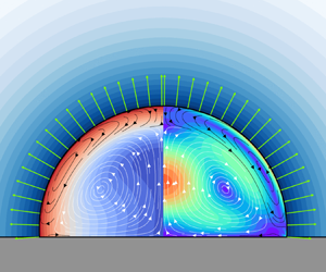
Figure 2. Simulation of a  ${1}\ {\mathrm {\mu }}\textrm {l}$ glycerol–water droplet revealing rich flow patterns during the evaporation process. The water vapour mass fraction is shown in the gas phase, whereas the glycerol mass fraction (left) and the velocity magnitude (right) are shown inside the droplet. (a) Initially, both Rayleigh and Marangoni convection support the flow from the apex to the contact line. (b) Although the contact angle is still above $\theta >{90}^{\circ }$, a Marangoni-induced counter-rotating vortex (black) emerges close to the interface, whereas the bulk flow is driven by natural convection (white). (c) Due to the increased evaporation rate at the contact line for $\theta <{90}^{\circ }$, the Marangoni-driven vortex grows in size until (d) the vortex driven by natural convection disappears. See supplementary movie 1 available at https://doi.org/10.1017/jfm.2020.734 for the entire simulation.
Initially, in figure 2(a), one can see a single vortex in the entire droplet, directed from the apex towards the contact line. This vortex is generated for two reasons, namely Marangoni convection and natural convection (Rayleigh convection). Due to the enhanced evaporation rate of water at the apex at the high contact angle, the water content is predominantly reduced at the top of the droplet, resulting in a lower surface tension compared to the region near the contact line. This drives a Marangoni flow towards the contact line. Since glycerol is more dense than water, the glycerol-rich outer shell of the droplet also sinks down due to natural convection, which also results in a flow from the apex to the contact line due to the spherical geometry. Hence, both mechanisms support recirculating flow in the same direction.
Remarkably, in figure 2(b), the situation changes. The contact angle is still above  ${90}^{\circ }$, i.e. the highest water evaporation rate is still at the top of the droplet. According to the aforementioned discussion, one would still naively expect the same kind of single-vortex flow. However, the simulation clearly shows two vortices, one in the bulk driven by natural convection (white) and another one close to the interface, which is driven by Marangoni flow in the opposite direction (black). The reason why the Marangoni flow is reversed, i.e. why there is more water at the top of the droplet although the evaporation rate of water is still dominant at the apex, is the fact that there is enhanced water replenishment by diffusion at the apex, which compensates for the rather small difference in the evaporation rates at the top and near the contact line. This can be seen by the rather steep concentration gradient in the normal direction at the apex compared to the region near the contact line. The reason for the steep concentration gradient in the normal direction close to the apex is the upward directed convective water replenishment from the bulk, which is governed by the internal vortex driven by natural convection. This means that sufficiently strong natural convection in the bulk can reverse the Marangoni flow at the interface, although one would not anticipate this by just considering the profile of the evaporation rate at this contact angle.
Upon further evaporation, in figure 2(c), the contact angle falls below  ${90}^{\circ }$, resulting in a higher water evaporation rate near the contact line. Hence, less water is present at the contact line as compared to the apex due two facts, namely, the effect of preferential evaporation at the contact line and the lower replenishing diffusive flux of water from the bulk at the contact line. Thereby, the Marangoni flow gets enhanced compared to the situation in figure 2(b) and the relative size of the Marangoni-induced vortex at the interface grows at the expense of the counter-rotating bulk vortex by natural convection.
Finally, in figure 2(d), the contact angle becomes rather small so that the Marangoni flow at the interface is even stronger due to the enhanced non-uniformity of the evaporation rate. Furthermore, the influence of natural convection also diminishes rather quickly, i.e. with cubic power in terms of the length scale according to the Rayleigh number (see later for its definition), due to the reduced volume of the droplet. This results in the depicted situation, i.e. that the flow direction within the entire droplet is completely determined by the Marangoni effect.
In a nutshell, one can infer from the direct numerical simulation results in figure 2 that there can be multiple flow scenarios during the drying of a single binary droplet, driven by an interplay of natural (i.e. Rayleigh) convection and Marangoni convection. One also clearly sees that, for a particle laden droplet, the coffee-stain effect would not occur as there is no noticeable flow towards the contact line (which for pure evaporating droplets transports the suspended particles to the rim of the pinned droplet) as compared to the strongly recirculating flow due to Marangoni flow and gravity.
4. Quasi-stationary approximation of the dynamical equations
After discussing some possible flow scenarios by considering a representative numerical example in the previous section, we will now focus on a simplification of the full model described in § 2. We generalize again from the particular case of a water–glycerol droplet to the general case of a binary droplet, where both liquids  ${A}$ and ${B}$ are allowed to evaporate. The goal is to find the simplest model possible that allows one to predict the expected flow scenario in the droplet by a minimum number of non-dimensional quantities.
4.1. Evaporation numbers
As shown in the example simulation, the liquid recirculates multiple times during the evaporation process due to the fast flow in the droplet. Hence, the typical liquid velocity  $\boldsymbol {u}$ is much larger than the normal interface movement velocity $\boldsymbol {u}_{{I}}$. Moreover, this leads to a rather well-mixed droplet, i.e. with typical compositional deviations of approximately a few per cent in terms of mass fractions, which can be attributed to the considerable Péclet number inside the droplet. These observations allow for several simplifications of the model. First of all, the liquid composition is expanded into two terms, i.e. $y_{{A}}(\boldsymbol {x},t)=y_{{A},0}+y$, namely the spatially averaged composition $y_{{A},0}$, which slowly evolves over the entire drying time, and the small local composition deviations $y(\boldsymbol {x},t)$. Since the composition-dependent liquid properties are usually rather smooth functions of the composition, this separation can be transferred to a first-order Taylor expansion of the liquid properties, i.e.
 \begin{equation} \left.\begin{gathered} \rho=\rho_0+y\partial_{y_{A}}\rho, \quad \sigma=\sigma_0+y\partial_{y_{A}}\sigma,\\ \mu=\mu_0+y\partial_{y_{A}}\mu,\quad D=D_{0}+y\partial_{y_{A}}D, \\ c_{{A}}^{{eq}}=c_{{A},0}^{{eq}}+y\partial_{y_{A}}c_{{A}}^{{eq}} , \quad c_{{B}}^{{eq}}=c_{{B},0}^{{eq}}+y\partial_{y_{A}}c_{{B}}^{{eq}} . \end{gathered}\right\} \end{equation}
Since the averaged composition  $y_{\text {A},0}$ evolves slowly, this expansion can be done at any specific time of interest during the evaporation process. In particular, this means that the coefficients of the Taylor expansions (4.1) can be treated as constants during some time close to the considered instant. This allows us to introduce the following non-dimensionalized scales
 \begin{equation} \boldsymbol{x}=V^{1/3}\tilde{\boldsymbol{x}},\quad t=\frac{V^{2/3}}{D_{0}}\tilde{t},\quad \boldsymbol{u}=\frac{D_{0}}{V^{1/3}}\tilde{\boldsymbol{u}} , \end{equation}
where the spatial scale is chosen in that way such that the non-dimensionalized droplet volume  $\tilde {V}$ becomes unity.
Of course, the introduced scales are only constant for a short instant in time, since the droplet volume  $V$ will decrease over time and the averaged mass fraction $y_{{A,0}}$ will change, resulting in varying Taylor expansions of the liquid properties. However, later in § 4.4, it is argued that the process can be considered to be quasi-stationary at each instant of the drying time. Thereby, the following non-dimensionalization and characteristic numbers are only valid for a specific considered instant of the drying time.
In a next step, the vapour fields are decomposed in a similar manner as (4.1), namely into a normalized contribution  $\tilde {c}_0$ which is one at the interface and zero at infinity and a contribution $\tilde {c}_\varDelta$ accounting for the effect of local composition variations on the vapour concentration via Raoult's law to the first order, i.e.
 \begin{equation} c_{\alpha}=(c_{\alpha,0}^{{eq}}-c_{\alpha}^{\infty})\tilde{c}_0 + c_{\alpha}^{\infty} + (\partial_{y_{A}}c_{\alpha}^{{eq}})\tilde{c}_\varDelta . \end{equation}
The Laplace equation (2.1) splits into two Laplace equations, i.e.  $\tilde {\nabla }^{2} \tilde {c}_0=0$ and $\tilde {\nabla }^{2} \tilde {c}_\varDelta =0$ and the boundary conditions (2.3) are transformed to
 \begin{equation} \tilde{c}_0=1\text{ and }\tilde{c}_\varDelta=y \quad \text{at the liquid--gas interface and} \end{equation}
 \begin{equation}\tilde{c}_0=\tilde{c}_\varDelta=0 \quad \text{far away from the droplet}. \end{equation}
Thereby, the evaporation rates (2.4) separate in the same way, i.e.
 \begin{equation} j_{\alpha}=\frac{D_{\alpha}^{{vap}}}{V^{1/3}}\big[(c_{\alpha,0}^{{eq}}-c_{\alpha}^{\infty})\tilde{j}_0 + (\partial_{y_{A}}c_{\alpha}^{{eq}})\tilde{j}_y\big], \end{equation}
where  $\tilde {j}_0=-\tilde \partial _n\tilde {c}_0$ only depends on the shape of the droplet, i.e. resembles the normalized evaporation profile of a homogeneous droplet, and $\tilde {j}_y=-\tilde {\partial }_n\tilde {c}_\varDelta$ is a nonlocal linear operator applied on $y$, i.e. the Dirichlet-to-Neumann map, accounting for deviations in the evaporation rate due to a varying interfacial composition via the composition-dependent vapour–liquid equilibrium, i.e. Raoult's law.
When dropping terms of quadratic order in  $y$, the convection–diffusion equation (2.5) within the droplet becomes
 \begin{equation} \partial_{\tilde t} y_{{A},0} + \partial_{\tilde t} y + \tilde{\boldsymbol{u}}\boldsymbol{\cdot}\tilde{\boldsymbol{\nabla} }y = \tilde{\nabla}^{2} y, \end{equation}
and the corresponding interface boundary condition (2.7) reads
 \begin{equation} -\!\tilde{\boldsymbol{\nabla}}y\boldsymbol{\cdot} \boldsymbol{n}= {Ev}_y\tilde{j}_0 +{Ev}_{{vap}}\tilde{j}_y - {Ev}_{{tot}} y \tilde{j}_0, \end{equation}
with the non-dimensional evaporation numbers
 \begin{gather} {Ev}_y=\frac{1}{\rho_0D_{0}}[(1-y_{{A},0})D_{{A}}^{{vap}}(c_{{A},0}^{{eq}}-c_{{A}}^{\infty})-y_{{A},0}D_{{B}}^{{vap}}(c_{{B},0}^{{eq}}-c_{{B}}^{\infty})], \end{gather}
 \begin{gather}{Ev}_{{vap}}=\frac{1}{\rho_0D_{0}}[(1-y_{{A},0})D_{{A}}^{{vap}}\partial_{y_{A}}c_{{A}}^{{eq}} -y_{{A},0}D_{{B}}^{{vap}}\partial_{y_{A}}c_{{B}}^{{eq}}], \end{gather}
 \begin{gather}{Ev}_{{tot}}=\frac{1}{\rho_0D_{0}}[D_{{A}}^{{vap}}(c_{{A},0}^{{eq}}-c_{{A}}^{\infty}) +D_{{B}}^{{vap}}(c_{{B},0}^{{eq}}-c_{\text{B}}^{\infty})]. \end{gather}
The number  ${Ev}_y$ quantifies the intensity of the concentration gradient induced in the liquid by preferential evaporation of one of the components, i.e. it compares the differences of the two diffusive vapour transports in the gas phase with the mutual diffusion in the binary liquid. Since the resulting composition gradient along the interface and in the bulk is the driving mechanism for Marangoni flow and natural convection, this number will become important to quantify these processes later on. Note that dependence on the volatilities of the components and their mass fractions in the liquid, ${Ev}_y$ may be positive or negative.
The parameter  ${Ev}_{{vap}}$ is an estimate for the influence of local variations in the liquid concentration on the preferential evaporation, i.e. the linear feedback due to the quasi-stationary diffusion in the gas phase. If the composition is rather uniform in the droplet, which is usually by fast recirculating convection, the term ${Ev}_{{vap}}\tilde {j}_y$ provides only a minor contribution in (4.8), meaning that the profile of the evaporation rates is similar to the one of a pure droplet. Since $\partial _{y_{A}}c_{{A}}^{{eq}}>0$ and $\partial _{y_{A}}c_{{B}}^{{eq}}<0$, i.e. the vapour concentration of $A$ increases and $B$ decreases for an increasing fraction of $A$ in the liquid, ${Ev}_{{vap}}$ is always positive. Large values of ${Ev}_{{vap}}$ can actually arise towards the end of the drying of a glycerol–water droplet, as discussed later in § 6.
Finally,  ${Ev}_{{tot}}$ is a measure for the total evaporation speed, i.e. for the typical interface speed $\tilde {\boldsymbol {u}}_{{I}}$ and the volume evolution. Note that the total evaporation speed and volume evolution are measures of the flow towards a pinned contact line, i.e. the flow leading to the coffee-stain effect. If none of the components condenses, i.e. both either evaporate or are non-volatile, the modulus of ${Ev}_y$ is smaller than ${Ev}_{{tot}}$. Nevertheless, since the deviation from the average composition is small, i.e. $y\ll 1$, and the Marangoni convection and/or natural convection are sufficiently large, the contribution of the latter to the flow can still be dominant compared to ${Ev}_{{tot}} y \tilde {j}_0$ in (4.8).
The evaporation numbers can be considered as Péclet numbers, e.g. the number  ${Ev}_{{tot}}$ actually compares the velocity of the interface motion due to evaporation to the liquid diffusion.
4.2. Non-dimensionalized flow
For the Navier–Stokes equations, we employ the established Boussinesq approximation, which is valid as long as  $y\partial _{y_{A}}\rho$ is small compared to $\rho _0$ (Gray & Giorgini Reference Gray and Giorgini1976). Due to the usually small composition gradients, this assumption is valid here. Therefore, except for the bulk force term $\rho g \boldsymbol {e}_z$, only the zeroth-order terms proportional to $\rho _0$ are kept, whereas $y\partial _{y_{A}}\rho$-terms are disregarded. With the same argument, terms proportional to $y\partial _{y_{A}}\mu$ and $y\partial _{y_{A}}\sigma$ can be disregarded whenever there is a dominant term proportional to $\mu _0$ or $\sigma _0$, respectively. Following this argument, the Navier–Stokes equations can be written as
 \begin{gather} {Sc}^{{-}1}(\partial_{\tilde{t}}\tilde{\boldsymbol{u}}+\tilde{\boldsymbol{u}}\boldsymbol{\cdot} \tilde{\boldsymbol{\nabla}}\tilde{\boldsymbol{u}})={-}\tilde{\boldsymbol{\nabla}} \tilde{p}+ \tilde{\boldsymbol{\nabla}}\boldsymbol{\cdot} (\tilde{\boldsymbol{\nabla}} \tilde{\boldsymbol{u}} + (\tilde{\boldsymbol{\nabla}} \tilde{\boldsymbol{u}})^{t} ) + {Ra}^{*} y \boldsymbol{e}_z, \end{gather}
 \begin{gather}\tilde{\boldsymbol{\nabla}}\boldsymbol{\cdot}\tilde{\boldsymbol{u}}=0. \end{gather}
Here, the shifted non-dimensionalized pressure, the Schmidt number and the starred Rayleigh number read
 \begin{equation} \tilde{p}=\frac{V^{2/3}}{D_{0}\mu_0}\left(p-\rho g z\right) , \quad {Sc}=\frac{\mu_0}{D_{0}\rho_0}, \quad {Ra}^{*}=\frac{V g\partial_{y_{A}}\rho}{D_{0}\mu_0}. \end{equation}
The Schmidt number for liquids is usually  ${Sc}>10^{3}$ which suggests that the left-hand side of (4.12) can be disregarded. However, since the chosen velocity and time scale in (4.2a–c) do not necessarily coincide with the actual present scales, this argument is only valid for small Reynolds numbers. In small droplets with rather low volatilities and regular Marangoni flow, however, this assumption is surely met, e.g. ${Re} < 0.05$ in the case of the simulation in figure 2. The starred Rayleigh number ${Ra}^{*}$ deviates from the conventional definition of the Rayleigh number just by the lack of an estimate for the composition difference, i.e. a term like ${\rm \Delta} y_{}$. The dynamic boundary conditions at the interface, (2.10) and (2.11), read in the Boussinesq approximation
 \begin{gather} -\tilde{p}+\boldsymbol{n}\boldsymbol{\cdot}(\tilde{\boldsymbol{\nabla}} \tilde{\boldsymbol{u}} + (\tilde{\boldsymbol{\nabla}} \tilde{\boldsymbol{u}})^{t} )\boldsymbol{\cdot} \boldsymbol{n} = \frac{1}{{Ca}^{*}}\left(\tilde\kappa+{Bo}\,\tilde{z}\right), \end{gather}
 \begin{gather}\boldsymbol{n}\boldsymbol{\cdot}(\tilde{\boldsymbol{\nabla}} \tilde{\boldsymbol{u}} + (\tilde{\boldsymbol{\nabla}} \tilde{\boldsymbol{u}})^{t} ) \boldsymbol{\cdot} \boldsymbol{t} = {Ma}^{*} \tilde{\boldsymbol{\nabla}}_{t} y \boldsymbol{\cdot} \boldsymbol{t} . \end{gather}
Here, the non-dimensional number  ${Ca}^{*}$, the Bond number and the starred Marangoni number read
 \begin{equation} {Ca}^{*}=\frac{D_{0}\mu_0}{V^{1/3}\sigma_0}, \quad {Bo}=\frac{\rho_0 g V^{2/3}}{\sigma_0}, \quad {Ma}^{*}=\frac{V^{1/3}\partial_{y_{A}}\sigma}{D_{0}\mu_0}. \end{equation}
Note that the definition of the starred capillary number  ${Ca}^{*}$ does not coincide with the conventional definition of the capillary number, i.e. it does not consider the actually present typical velocity scale, i.e. the intensity of the capillary shape relaxations during evaporation cannot be inferred from ${Ca}^{*}$. However, both the real capillary number ${Ca}=\mu _0U/\sigma _0$ and ${Ca}^{*}$ are small in the systems considered here ( ${Ca}<1\times 10^{-6}$ and ${Ca}^{*}<1\times 10^{-7}$ in the simulation depicted in figure 2). Similar to ${Ra}^{*}$, the starred Marangoni number $\textit{Ma}^{*}$ lacks an estimate for the composition difference, i.e. ${\rm \Delta} y$, as compared to the conventional definition. Finally, the kinematic boundary condition (2.6) becomes
 \begin{equation} \left(\tilde{\boldsymbol{u}}-\widetilde{\boldsymbol{u}_{{I}}}\right) \boldsymbol{\cdot}\boldsymbol{n}={Ev}_{{tot}} \tilde{j}_0 + {Ev}_{{tot,vap}} \tilde{j}_y , \end{equation}
where
 \begin{equation} {Ev}_{{tot,vap}}=\frac{1}{\rho_0D_{0}}\left[D_{{A}}^{{vap}}\partial_{y_{A}}c_{{A}}^{{eq}} +D_{{B}}^{{vap}}\partial_{y_{A}}c_{{B}}^{{eq}}\right] \end{equation}
is the analogue of  ${Ev}_{{vap}}$ for the total evaporation rate, i.e. the effect of a change in the saturation pressure due to a locally deviating composition on the total evaporation rate.
4.3. Estimation of the outwards flow
Before focusing on natural convection and Marangoni flow in the droplet, it is beneficial to obtain an estimate for the velocity in the droplet in the absence of these mechanisms, i.e.  ${Ma}^{*}={Ra}^{*}=0$. This case, exemplified e.g. by a pure isothermal droplet, combined with a pinned contact line represents the purely capillary-driven outward flow, which causes the coffee-stain effect.
For small droplets, the capillary number  ${Ca}$ is small, so that the surface tension forces according to (4.15) lead to an intense relaxing traction whenever the droplet deviates from the equilibrium shape. Since the Bond number ${Bo}$ is small also for small droplets, the hydrostatic term in (4.15) can be neglected, leading to a spherical cap with a homogeneous curvature $\tilde {\kappa }$ as the equilibrium shape. Hence, the shape evolution and thereby the interface velocity $\widetilde {\boldsymbol {u}_{{I}}}$ are solely given by the evaporation rate and the contact line kinetics, which is assumed to be pinned here. Since the term ${Ev}_{{tot,vap}} \tilde {j}_y$ in (4.18) is proportional to $y$, it can be disregarded with respect to ${Ev}_{{tot}} \tilde {j}_0$ in accordance with the Boussinesq approximation. As a consequence, one ends up with a linear Stokes flow problem, where the entire bulk velocity is given by the instantaneous shape relaxation, which is proportional to the rate of evaporation, i.e. to ${Ev}_{{tot}}$.
By integrating the evaporation rate  ${Ev}_{{tot}} \tilde {j}_0$ one obtains the volume loss and thereby one can reconstruct the normal velocity of the interface $\tilde {\boldsymbol {u}}_{{I}}\boldsymbol {\cdot }\boldsymbol {n}$. The flow in the bulk $\tilde {\boldsymbol {u}}$ is subsequently given by solving the Stokes flow with the normal boundary condition $\tilde {\boldsymbol {u}}\boldsymbol {\cdot }\boldsymbol {n}=\widetilde {\boldsymbol {u}_{{I}}} \boldsymbol {\cdot }\boldsymbol {n}+{Ev}_{{tot}}\tilde {j}_0$. In figure 3, representative solutions for the bulk flow $\tilde {\boldsymbol {u}}$ with unity evaporation number, i.e. ${Ev}_{{tot}}=1$, are depicted. It is apparent that the typical bulk velocity is of the order of unity, i.e. $\|\tilde {\boldsymbol {u}}\|\sim 1$. Since the flow is proportional to ${Ev}_{{tot}}$, the typical velocity corresponding to an arbitrary evaporation number ${Ev}_{{tot}}$ is hence $\|\tilde {\boldsymbol {u}}\|\sim {Ev}_{{tot}}$. This holds also for the typical interface movement, i.e. $\|\tilde {\boldsymbol {u}}_{{I}}\|\sim {Ev}_{{tot}}$.

Figure 3. Bulk flow for small capillary number  ${Ca}$ and Bond number ${Bo}$ in the absence of Marangoni flow and natural convection for a total evaporation number ${Ev}_{{tot}}=1$ and contact angles of (a) $\theta ={60}^{\circ }$ and (b) $\theta ={120}^{\circ }$. The evaporation rate ${Ev}_{{tot}}\tilde {j}_0$ causes a volume loss, which prescribes the normal interface movement $\tilde {\boldsymbol {u}}_{{I}}\boldsymbol {\cdot }\boldsymbol {n}$ (depicted on the left sides). The bulk flow (right sides) is governed by Stokes flow with the normal boundary condition $\tilde {\boldsymbol {u}}\boldsymbol {\cdot }\boldsymbol {n}= \widetilde {\boldsymbol {u}_{{I}}}\boldsymbol {\cdot }\boldsymbol {n}+{Ev}_{{tot}}\tilde {j}_0$. Apparently, the typical purely capillary-driven velocity is of order ${Ev}_{{tot}}$.
4.4. Quasi-stationary limit
Knowing that the capillary flow due to the volume loss is of the order of  ${Ev}_{{tot}}$, we now focus on the contributions to the flow by Marangoni forces and natural convection. In a first step, one can consider the case where ${Ev}_{{tot}}=0$, i.e. no total mass transfer and hence a constant volume and shape of the droplet. This scenario can be realized by tuning the ambient humidities of $A$ and $B$ so that the evaporative mass loss of component $A$ is balanced by the condensation of component $B$. In this case ${Ev}_{{tot}}=0$ and ${Ev}_y>0$ holds. Again, due to the small capillary number and the small Bond number, one can assume a spherical cap shape with volume $\tilde {V}=1$ and contact angle $\theta$, which are both constant now. Furthermore, there is no interface movement, $\tilde {\boldsymbol {u}}_{{I}}\boldsymbol {\cdot }\boldsymbol {n}=0$, and no total mass transfer, $\tilde {\boldsymbol {u}}\boldsymbol {\cdot }\boldsymbol {n}=0$.
By averaging (4.7) over the droplet volume  $\tilde {V}=1$, defining the integrated evaporation rate
 \begin{equation} \tilde{J}=\int \tilde{j}_0 \,\mathrm{d}\tilde{A} \end{equation}
and considering only the zeroth-order term in the boundary condition (4.8) in accordance with the Boussinesq approximation, one can separate the average composition  $y_{{A},0}$ and the deviation $y$ as follows:
 \begin{gather} \partial_{\tilde{t}} y_{{A},0} ={-}{Ev}_y \tilde{J}_0, \end{gather}
 \begin{gather}\partial_{\tilde{t}} y + \tilde{\boldsymbol{u}}\boldsymbol{\cdot}\tilde{\boldsymbol{\nabla}} y = \tilde{\nabla}^{2} y +{Ev}_y \tilde{J}_0 . \end{gather}
Here, the term  ${Ev}_y \tilde {J}_0$ assures that $y_{{A},0}$ is indeed the average composition and that the average of $y$ remains zero, i.e. the term compensates for the imposed composition gradient at the liquid–gas interface. As already stated in § 4.1, this splitting holds only for a limited time, since a variation in $y_{{A},0}$ leads to a change in the liquid properties which were used for the non-dimensionalization. Usually, however, the coupled dynamics of flow $\tilde {\boldsymbol {u}}$ and compositional differences $y$ due to Marangoni and natural convection is considerably faster than ${Ev}_y \tilde J_0$, This was already apparent from the simulations depicted in figure 2 and it will be validated later in § 6. Furthermore, this observation allows us to focus on stationary solutions. Finally, upon introducing
 \begin{equation} \xi =\frac{y}{{Ev}_y}, \end{equation}
one ends up at the following set of coupled equations:
 \begin{gather} \tilde{\boldsymbol{u}}\boldsymbol{\cdot}\tilde{\boldsymbol{\nabla}} \xi = \tilde{\nabla}^{2} \xi +\tilde{J}_0, \end{gather}
 \begin{gather}-\tilde{\boldsymbol{\nabla}} \tilde{p} + \tilde{\boldsymbol{\nabla}}\boldsymbol{\cdot} (\tilde {\boldsymbol{\nabla}} \tilde{\boldsymbol{u}} + (\tilde{\boldsymbol{\nabla}} \tilde{\boldsymbol{u}})^{t} ) + {Ra}\, \xi \boldsymbol{e}_z=0, \end{gather}
 \begin{gather}\tilde{\boldsymbol{\nabla}}\boldsymbol{\cdot}\tilde{\boldsymbol{u}}=0, \end{gather}
subject to the following boundary conditions:
 \begin{gather} -\tilde{\boldsymbol{\nabla}}\xi\boldsymbol{\cdot} \boldsymbol{n}= \tilde{j}_0, \end{gather}
 \begin{gather}\tilde{\boldsymbol{u}}\boldsymbol{\cdot}\boldsymbol{n}=0, \end{gather}
 \begin{gather}\boldsymbol{n}\boldsymbol{\cdot}(\tilde{\boldsymbol{\nabla}} \tilde{\boldsymbol{u}} + (\tilde{\boldsymbol{\nabla}} \tilde{\boldsymbol{u}})^{t} ) \boldsymbol{\cdot} \boldsymbol{t} = {Ma}\,\tilde{\boldsymbol{\nabla}}_{t} \xi \boldsymbol{\cdot} \boldsymbol{t} \end{gather}
at the liquid–gas interface and
 \begin{gather} \tilde{\boldsymbol{\nabla}}\xi\boldsymbol{\cdot} \boldsymbol{n}= 0, \end{gather}
 \begin{gather}\boldsymbol{u}=0 \end{gather}
at the liquid–substrate interface. Note that the simplified kinematic boundary condition (4.28) is now compatible with the no-slip boundary condition (4.31) at the contact line, i.e. a slip length is not required. Since the mesh is static, the Laplace pressure (2.10) need not to be imposed. Equation (4.28) is enforced via a Lagrange multiplier field at the interface. Hence, any in- or outflow through the interface is prevented by adjusting the local normal traction accordingly.
Besides the contact angle  $\theta$, only two parameters enter the system, namely the Marangoni number and the Rayleigh number, which read
 \begin{equation} {Ma}={Ma}^{*}{Ev}_y=\frac{V^{1/3}\partial_{y_{A}}\sigma}{D_{0}\mu_0}{Ev}_y,\quad {Ra}={Ra}^{*}{Ev}_y=\frac{V g\partial_{y_{A}}\rho}{D_{0}\mu_0}{Ev}_y. \end{equation}
Note that the characteristic numbers for both mechanisms are proportional to the induced composition gradient due to mass transfer, i.e.  ${Ev}_y$. Of course, in particular the tangential gradient along the interface is also strongly dependent on the contact angle $\theta$, since this determines the profile of the evaporation rate $\tilde {j}_0$.
These equations are not only valid for the specific assumed case of  ${Ev}_{{tot}}=0$, but also when the combination of Marangoni and Rayleigh flow $\tilde {\boldsymbol {u}}$ predicted by this model is considerably faster than the capillary flow, i.e. a flow situation with outwards flow leading to the coffee-stain effect. According to the estimations in § 4.3, this is the case if $\tilde {\boldsymbol {u}}\gg {Ev}_{{tot}}$.
5. Phase diagram for combined Marangoni and Rayleigh convection
5.1. Procedure
Unfortunately, the analytical treatment of the model equations (4.24)–(4.26) is hampered by the geometry, which demands rather complicated toroidal coordinates, and by the very strong nonlinear coupling of  $\tilde {\boldsymbol {u}}$ and $\xi$ due to the advection term. Therefore, we investigate the system by numerical means. Our analysis is limited to axisymmetric solutions and we only consider the case ${Ev}_{{vap}}=0$, i.e. neglecting the feedback of the altered gas composition due to the liquid–vapour equilibrium on the local evaporation rate. Finally, we will focus on the case ${Ma} \geqslant 0$, for which evaporation leads to an overall reduction of the surface tension, as in the case of the water–glycerol depicted in figure 2. This results in a regular flow, i.e. no chaotic behaviour can be found, at least not for moderate flow conditions. In the case of negative Marangoni numbers, chaotic flow patterns cannot be excluded due to the Marangoni instability (Machrafi et al. Reference Machrafi, Rednikov, Colinet and Dauby2010; Christy et al. Reference Christy, Hamamoto and Sefiane2011; Bennacer & Sefiane Reference Bennacer and Sefiane2014). Of course, this spatio-temporal evolving type of flow cannot be captured within the assumption of a quasi-stationary process. One can, on the other hand, test the linear stability of the quasi-stationary solutions in the case of negative Marangoni numbers to find the transition to chaotic flow, but since also the axial symmetry is usually broken in the case of negative Marangoni numbers, one also would have to generalize the entire solution procedure from axisymmetric cylindrical coordinates to the full three-dimensional problem, as done by Diddens et al. (Reference Diddens, Tan, Lv, Versluis, Kuerten, Zhang and Lohse2017b). The transition into chaotic flow still remains to be investigated in detail, but the three-dimensional numerical results of Diddens et al. (Reference Diddens, Tan, Lv, Versluis, Kuerten, Zhang and Lohse2017b) indeed show that the route to chaos happens via a breaking of the axial symmetry, similarly to what is seen in the case of intense thermal Marangoni flow in a pure droplet (Sefiane et al. Reference Sefiane, Moffat, Matar and Craster2008).
In order to find solutions of the system, we employed a finite element method on an axisymmetric mesh with triangular elements. We used linear basis functions for  $\xi$ and $\tilde {p}$ and quadratic basis functions for $\tilde {\boldsymbol {u}}$, i.e. typical Taylor–Hood elements. The equations have been implemented in both FEniCS (https://fenicsproject.org/) (Logg et al. Reference Logg, Mardal and Wells2012) and oomph-lib for mutual validation. The condition of zero velocity in the normal direction, i.e. (4.28), has been implemented by Lagrange multipliers. For an enhanced stability in the Newton method during the solution process, it has been found beneficial to replace $\tilde {J}_0$ in (4.24) by a Lagrange multiplier which ensures that the average of $\xi$ is zero. This removes the null space with respect to a constant shift in $\xi$ and a corresponding adjustment of the pressure $\tilde {p}$.
Due to the nonlinear advection term, it is in general possible that multiple solutions exist for a given parameter combination  $(\theta ,{Ma},{Ra})$. For the parameter ranges considered in the following, however, we are confident that we found the generic solutions due to the following strategy: for every considered contact angle $\theta$, we performed adiabatic scans along ${Ra}$ in the increasing and decreasing directions for fixed ${Ma}$ and vice versa. During that, no hysteresis, i.e. bistable regions, have been found. Furthermore, by tracing these parameter paths with continuation, we have not detected any unstable branches. This has been furthermore validated by investigating the eigenvalues with a shift-inverted Arnoldi method (using Spectra https://spectralib.org). Finally, for each parameter combination, we performed temporal integrations of the unsteady model equations starting from a homogeneous state $\xi =0$. Since these runs converged to the same solutions as obtained by the steady parameter scans, we are sure that all solutions discussed in the following are indeed generic and stable. Note, however, that this is in general not true outside the considered parameter ranges.
5.2. Phase diagrams
The phase diagrams for small and large contact angles, i.e. for  $\theta ={60}^{\circ }$ and $\theta ={120}^{\circ }$, are depicted in figures 4 and 5, respectively. Here we have assumed, as in the case of the glycerol–water droplet, that the blue liquid $A$ (e.g. water) is more volatile, less dense but associated with a higher surface tension than the red liquid $B$ (e.g. glycerol). This means by definition that ${Ma}>0$ holds and that a sessile droplet is described by ${Ra}>0$ whereas a pendant droplet is given by ${Ra}<0$. While in the diagrams (figures 4 and 5) a negative Rayleigh number is always indicated by a pendant droplet, it can also be realized by changing the sign of $\partial _y \rho$, i.e. by letting the red component be lighter than the blue component.

Figure 4. Qualitative flow types as functions of the Marangoni number  ${Ma}$ and the Rayleigh number ${Ra}$ for a small contact angle $\theta =60^{\circ }$. For sessile droplets ( ${Ra}>0$) with large Marangoni numbers and small Rayleigh numbers, Marangoni flow dominates in the droplet and results in a circulating flow from the contact line along the free interface towards the apex (Ma dominant, black streamlines). On the contrary, if ${Ma}$ is small and ${Ra}$ is large, gravity-driven flow dominates with a flow direction from the apex along the free interface to the contact line (Ra dominant, white streamlines). While the other mechanism, i.e. natural convection in the regime Ma dominant and Marangoni flow in the regime Ra dominant, can still quantitatively influence the flow, only a single vortex can be found which is driven by the dominant mechanism. In between these regions, however, there is a regime where the bulk flow is driven by natural convection whereas the flow close to the interface is dominated by the Marangoni effect (Ma vs. Ra). Here, two counter-rotating vortices can be seen. For pendant droplets ( ${Ra}<0$), both mechanisms driving the flow in the same direction (Ma and Ra same direction). Hence, one cannot identify the main driving mechanism from the direction of the flow, so that the streamlines are coloured grey. If both mechanisms are sufficiently strong, however, the bulk flow due to natural convection can become so intense that the composition gradient along the interface changes direction and a flow reversal due to the Marangoni effect can arise in the vicinity of the interface (Ra reverses Ma).

Figure 5. Qualitative flow types as functions of the Marangoni number  ${Ma}$ and the Rayleigh number ${Ra}$ for a high contact angle $\theta =120^{\circ }$. Since the direction of the Marangoni flow is reversed in comparison to the case $\theta <90^{\circ }$ (cf. figure 4), the diagram qualitatively flips upside down. Now, for sessile droplets ( ${Ra}>0$) both mechanisms act in the same direction (Ma and Ra same direction) and for sufficiently intense driving, the natural convection in the bulk can reverse the composition gradient at the interface, leading to a Marangoni-driven reversal close to the interface (Ra reverses Ma). For pendant droplets ( ${Ra}<0$), either Marangoni flow or natural convection dominates (Ma dominant/Ra dominant), or the bulk flow is driven by natural convection, whereas the interfacial flow is governed by Marangoni flow (Ma vs. Ra).
Depending on the Marangoni number  ${Ma}$, the Rayleigh number ${Ra}$ and the contact angle $\theta$, different qualitative flow scenarios can be found. For high Marangoni numbers and small Rayleigh numbers, the Marangoni flow dominates (Ma dominant) and vice versa (Ra dominant). In between, however, for sessile droplets with a contact angle below ${90}^{\circ }$ and for pendant droplets with a contact angle above ${90}^{\circ }$, there is a region where the Marangoni effect determines the flow direction at the interface, whereas the bulk flow is driven by natural convection (Ma vs. Ra). In the opposite cases, i.e. for pendant droplets with $\theta <{90}^{\circ }$ and sessile droplet with $\theta >{90}^{\circ }$, both mechanisms drive a flow in the same direction, so that one cannot directly distinguish between the two mechanisms driving the flow (Ma and Ra same direction). In the limit of very strong driving of both mechanisms, however, natural convection can become so intense that the surface tension gradient is reversed, leading to a Marangoni-induced reversal of the flow at the interface (Ra reverses Ma). This effect can be explained by the distortion of the internal composition field due to natural convection. For pendant droplets with $\theta <{90}^{\circ }$, the composition gradient in the bulk in normal direction is much more pronounced near the contact line as opposed to the apex. As a consequence, the diffusive replenishment of the blue liquid at the interface is enhanced near the contact line so that in fact more blue liquid, i.e. the one with higher surface tension, can be found near the contact line instead of at the apex – despite of its higher volatility and the pronounced evaporation rate at the contact line. The resulting Marangoni flow is therefore reversed as anticipated by considering the profile of the evaporation rate alone. The same explanation holds for the case $\theta >{90}^{\circ }$, except that one finds a more pronounced normal composition gradient near the apex as compared to the region close to the contact line, and the situation is reversed.
All transitions between the aforementioned regimes are continuous. The drawn phase boundaries are defined by the emergence or disappearance of a second vortex. There is no bifurcation and/or hysteresis present at the boundaries of the regimes. In supplementary movie 2, a path through the parameter space is traversed and the corresponding stationary solution is shown, which illustrates the behaviour of the flow upon crossing the phase region boundaries, i.e. how the stationary solution gradually changes between single- and two-vortex solutions.
Finally, we also investigate the contact angle dependence of the phase diagrams by showing the corresponding regions for  $\theta ={40}^{\circ }$, ${60}^{\circ }$ and ${80}^{\circ }$ in figure 6(a) and for $\theta ={100}^{\circ }$, ${120}^{\circ }$ and ${140}^{\circ }$ in figure 6(b). Obviously, the phase boundaries are shifted, but qualitative differences in the phase diagrams cannot be found.

Figure 6. Influence of the contact angle  $\theta$ on the boundaries of the phase diagram for (a) $\theta <{90}^{\circ }$ and (b) $\theta >{90}^{\circ }$. (Ra rev. Ma: Ra reverses Ma.)
In the special case of  $\theta ={90}^{\circ }$, the profile of the evaporation rate is uniform along the droplet. Hence, Marangoni flow cannot be induced by preferential evaporation. Since ${Ma}>0$ is considered throughout this article, the Marangoni flow is stable, i.e. in the absence of natural convection ( ${Ra}=0$), only radial diffusion is observed in our simulations. For non-vanishing, but even for small Rayleigh numbers, the bulk flow is governed by natural convection (i.e. absence of the Ma-dominant regime). For sufficiently high Marangoni numbers, this natural convection induces a counter-rotating Marangoni vortex in the vicinity of the interface (Ma-vs-Ra regime).
Note again that we have assumed in the phase diagrams that the more volatile liquid (blue) is less dense in the insets in the phase diagrams. In the other case, the droplets depicted in the insets are required to be mirrored vertically, as the Rayleigh number is then negative for sessile droplets and positive for pendant droplets. Furthermore, it is noteworthy that these diagrams are for pinned droplets (CR-mode) and droplets with a constant contact angle (CA-mode), as only stationary solutions are considered anyway. As long as the dominant velocity contribution is given by recirculating flow due to Marangoni and/or natural convection, any capillary flow due to shape relaxations can be disregarded. Finally, the diagrams can also be used for condensation instead of evaporation, as long as  ${Ma}>0$ holds. For condensation of component $A$,
$A$,  ${Ev}_y<0$ holds, so that ${Ma}>0$ is true if component $A$ has the lower surface tension, i.e. $\partial _{y_{A}}\sigma <0$. We therefore anticipate that the diagrams can predict the flow when ethanol condenses on a pure water droplet, whereas it would fail to predict the flow when water condenses on a pure glycerol droplet ( ${Ma}<0$). In fact, the latter case has been investigated experimentally, showing indeed chaotic cellular flow structures (Shin, Jacobi & Stone Reference Shin, Jacobi and Stone2016).
6. Validation of the quasi-stationary approximation against the full numerical simulation
Since there were a number of assumptions made in the simplification of the problem, it is necessary to validate the predicted flow by comparing it with results of the full numerical simulation, i.e. with the full set of equations as described in § 2. We focus on the representative simulation depicted in figure 2. At each instant in time, we have extracted the spatially averaged water mass fraction  $y_{{A},0}$, the volume $V$ to determine the spatial scale $\sqrt [3]{V}$ and the contact angle $\theta$ from the simulation. Using the composition-dependent properties of binary glycerol–water mixtures, we can obtain $\rho _0=\rho (y_{{A},0})$, $\mu _0=\mu (y_{{A},0})$, $D_0=D(y_{{A},0})$, $c_{{A},0}^{eq}=c_{{A}}^{eq}(y_{{A},0})$, $\sigma _0=\sigma (y_{{A},0})$ and the local slopes $\partial _{y_{A}} \rho$ and $\partial _{y_{A}} \sigma$ by the averaged composition $y_{{A},0}$ at each instant in time. This allows us to calculate the normalized evaporation-induced composition gradient ${Ev}_y$ and the characteristic numbers ${Ra}$ and ${Ma}$. On the basis of these numbers and the contact angle, we solve the simplified quasi-stationary model and re-dimensionalize the resulting velocity and composition field as well as the evaporation rate using the scales (4.2a–c). This procedure allows us to compare the full unsteady evolution of the droplet with the corresponding predictions at each instant by the simplified quasi-stationary model.
The results are depicted for several instants in figure 7, where the full simulation is shown on the left and the corresponding prediction of the quasi-stationary model is depicted on the right. Initially, i.e. in figure 7(a), the full simulation has not attained the quasi-stationary limit. Hence, the quasi-stationary model slightly overpredicts the composition variations, i.e. it shows more glycerol (red) near the interface and more water (blue) in the bulk. Therefore, the flow field also slightly differs, i.e. the transient full simulation shows a single vortex, whereas the quasi-stationary model predicts the presence of a small counter-rotating vortex near the apex. Furthermore, a very gentle deviation in the spherical cap shape due to the gravitational effect in the full simulation can be seen at the apex as well (regime Ra reverses Ma). At later time steps, i.e. in figure 7(b–d), however, the flow and the composition predicted by the quasi-stationary model match the results of the full simulation almost perfectly, be it in terms of the composition field, the flow pattern, the shape or the evaporation rate. This result substantiates the fact that the capillary outwards flow, which has been disregarded in the quasi-stationary model, can indeed be neglected as long as there is a prominent recirculating flow due to Marangoni and/or Rayleigh convection.

Figure 7. Comparison of the full simulation (left) from figure 2 and the corresponding result predicted by the quasi-stationary model (right) at different times. The colour code inside shows the glycerol concentration, whereas the streamlines indicate the velocity field. In the gas phase, the water vapour and the corresponding evaporation rate are depicted. (a) Initially, the full simulation has not yet attained the quasi-stationary limit, so that the intensity of the composition deviation is overpredicted in the quasi-stationary model. In (b–d), the quasi-stationary model predicts the result of the full simulation up to a deviation that can be barely seen by eye. See supplementary movie 3 for the comparison between full simulation and quasi-stationary model over the entire simulation time.
To assess the quality of the quasi-stationary model in more detail, we have extracted some characteristic quantities of both simulations, i.e. from the full simulation of figure 2 and the corresponding quasi-stationary limit at each instant. In figure 8(a), the time evolution of the three key parameters, namely the Rayleigh number  ${Ra}$, the Marangoni number ${Ma}$ and the contact angle $\theta$ is shown. These numbers were used as input for the quasi-stationary model. The root mean square (r.m.s.) of the velocity inside the droplet is depicted in figure 8(b). Again one can see an initial disagreement due to the fact that the full simulation has not yet attained its quasi-stationary limit. After that, i.e. after approximately ${50}\ \textrm {s}$ to ${100}\ \textrm {s}$, the r.m.s. velocity is well predicted until it shows again a disagreement towards the end of the drying time. The reason for the overpredicted velocity in the quasi-stationary model can be found in figure 8(c), where the minimum and maximum glycerol concentration in the droplet according to both simulations are plotted against time. While it shows good agreement in the main part of the drying, the quasi-stationary model shows an enhanced maximum glycerol concentration towards the end of the drying, i.e. when almost only glycerol is left in the droplet. In fact, the glycerol concentration predicted by the quasi-stationary model even exceeds the physically realistic threshold of 100 %. Obviously, this overprediction of the composition differences explains the elevated prediction of the r.m.s. velocity. The reason for the overpredicted composition difference can finally be seen in figure 8(d), where the evaporation numbers are depicted. When the droplet almost entirely consists of glycerol, the evaporation number $Ev_{vap}$, quantifying the reduction of the water vapour pressure for vanishing water at the interface on the evaporation dynamics (cf. (4.10)), becomes very large ( ${Ev}_{{vap}}\to 18$ at $t={1000}\ \textrm {s}$). This effect is not considered in the quasi-stationary model, since it assumes the averaged composition $y_{{A},0}$ to predict the vapour–liquid equilibrium, not the local composition at the interface. Thereby, the amount of water vapour is strongly overestimated which results in a high evaporation rate and thereby in an unrealistically high composition difference. Obviously, the quasi-stationary model loses validity when ${Ev}_{{vap}}$ becomes too large, meaning that the dependence of the vapour–liquid equilibrium on the local interface composition cannot be neglected anymore. For a more detailed model, this effect can easily be incorporated into the quasi-stationary model, but it would introduce a fourth parameter besides ${Ma}$, ${Ra}$ and $\theta$ into the set of equations, which is beyond the scope of this article.

Figure 8. Comparison of characteristic quantities of the full simulation of figure 2 and the corresponding results predicted by the quasi-stationary model. (a) The three input parameters for the quasi-stationary model  ${Ra}$, ${Ma}$ and $\theta$ extracted from the full simulation. (b) Comparison of the root-mean-square velocity. (c) Comparison of the maximum and minimum glycerol content inside the droplet. (d) Evaporation numbers extracted from the full simulation.
7. Conclusion
During the evaporation of a binary droplet, multiple flow scenarios can be found, which is a result of an interplay of differences in the volatilities, mass densities and surface tensions of the two constituents. The difference in the volatilities induces compositional gradients in the bulk and also, due to the in general non-homogeneous evaporation rate, along the interface. Due to the composition-dependent mass density and surface tension, natural convection and Marangoni flow can set in, leading to a recirculating flow in the droplet that is usually much faster than the typical capillary outwards flow towards the contact line, which can be seen in pure droplets and leads to the coffee-stain effect in particle-laden droplets.
Based on justified assumptions, we simplified the full model equations to a quasi-stationary model that only requires three parameters, namely the contact angle, the Rayleigh and the Marangoni number. Both, the Rayleigh and Marangoni number linearly scale with a non-dimensional evaporation number,  ${Ev}_y$, which is a measure for the induced composition gradient by the preferential evaporation of one or the other component. By numerically solving for stationary solutions of the simplified model, we have explored the phase space in terms of these three quantities. The obtained phase diagrams allow for the prediction of the flow types in sessile and pendant binary droplets, with contact angles below and above ${90}^{\circ }$.
We found in total five different flow patterns: if one of the mechanisms, i.e. either natural convection or Marangoni flow, becomes sufficiently strong as compared to the other one, it can dominate and control the flow direction in the entire droplet. This scenario can usually be seen in the case when one corresponding number, namely the Rayleigh or Marangoni number, respectively, is much larger than the other. In these cases, a single vortex can be seen in the droplet. If both mechanisms drive the flow into a different direction and are comparably strong in terms of their non-dimensional numbers, one can find two vortices, one in the bulk driven by natural convection, and a counter-rotating vortex at the interface due to Marangoni flow. The fourth flow type is the case, when both mechanisms act in the same direction, so that one cannot distinguish the particular cause of the driving and only a single vortex is present. Remarkably, however, in particular regimes in the phase space, the Marangoni flow can be reversed due to the natural convection in the bulk, leading to the fifth solution, where again two vortices can be found. In this situation, the bulk flow driven by natural convection deforms the internal composition field so that the diffusion dynamics in the liquid is altered, which eventually reverses the composition gradient at the interface and hence the Marangoni flow.
To use the phase diagrams presented in this article, several requirements have to be fulfilled: first of all, the influence of thermal effects must be negligible compared to the solutal ones. The two liquids must be miscible and the droplet must not be too large, so that the capillary number and the Bond number are small in order to guarantee a spherical cap shape during the evaporation. Furthermore, the Reynolds number must be small and the spatial variations in the composition must be small enough in order to allow for a first-order Taylor expansion of the composition-dependent liquid properties according to (4.1). Also the requirements for the Boussinesq approximation must hold. The Marangoni number, as defined in (4.32a,b), must be positive, i.e. evaporation leads to an overall decrease of the surface tension, so that Marangoni-unstable chaotic flow can be excluded and the recirculating flow must be sufficiently faster than the movement of the interface. Finally, the influence of a change in the local composition on the vapour–liquid equilibrium may not be too strong, as it has been discussed on the basis on the evaporation number  ${Ev}_{{vap}}$ describing the feedback of local composition changes on the evaporation rate in § 6.
If all these requirements are fulfilled and the composition dependence of the required physical properties are known, the phase diagrams of this article allow for a prediction of the qualitative flow pattern in an evaporating binary droplet, probably with the exception of a short initial transient phase.
The method described in this article can be directly transferred to thermally driven Marangoni flow and natural convection in a pure droplet. Instead of a convection–diffusion equation for one component, one would have to consider the convection–diffusion equation for the temperature field. The boundary conditions will be different, e.g. a Dirichlet boundary condition of constant temperature at a highly conducting substrate and non-dimensional evaporative cooling instead of the number  ${Ev}_y$, but the methodological principle can remain the same. Also, a generalization to negative Marangoni numbers could be interesting, but it would require consideration of the problem in three dimensions. This would allow us to predict axial symmetry breaking and also bifurcations into chaotic Marangoni flow regimes by performing a linear stability analysis of the quasi-stationary solutions.
Supplementary movies
Supplementary movies are available at https://doi.org/10.1017/jfm.2020.734.
Acknowledgements
This work is part of an Industrial Partnership Programme (IPP) of the Netherlands Organization for Scientific Research (NWO). This research programme is co-financed by Canon Production Printing Holding B.V., University of Twente and Eindhoven University of Technology. D.L. gratefully acknowledges support by his ERC-Advanced Grant DDD (project number 740479).
Declaration of interests
The authors report no conflict of interest.
Appendix A. Comparison with experiments and relation to the Grashof number
Since even the detailed full model is subject to some assumptions, e.g. diffusion-limited vapour transport and disregard of thermal effects, we also performed experiments on various sessile and pendant binary droplets with different volumes and contact angles. The details of the experimental set-up are described by Li et al. (Reference Li, Diddens, Lv, Wijshoff, Versluis and Lohse2019a). Here, we are more interested in a qualitative agreement, i.e. whether the flow direction is dominated by natural convection or not.
Simultaneously, we address the Grashof number (also known as the Archimedes number) in the following. This number, defined as
 \begin{equation} {Gr}=gh^{3}\rho_0(\rho_{A,pure}-\rho_{B,pure})/\mu^{2}, \end{equation}
with  $h$ being the height of the droplet and $\mu$ the averaged viscosity of the liquids, was used in our previous publication (Li et al. Reference Li, Diddens, Lv, Wijshoff, Versluis and Lohse2019a) as an indicator as to whether the flow in the droplet is dominated by natural convection ( ${Gr}\gg 1$) or not ( ${Gr}\ll 1$). Compared to the non-dimensional numbers presented in this manuscript, i.e. the evaporation number ${Ev}_y$ and the Rayleigh number ${Ra}$, this number is independent of the current droplet composition. Instead, it just takes the pure densities of both fluids and the averaged density and viscosity into account. This means that the Grashof number ${Gr}$ is easily accessible, whereas the non-dimensional numbers used throughout this manuscript require knowledge of the instantaneous average composition and the full composition dependence of all properties, which is not always possible in an experimental set-up.
Therefore, we are interested in substantiating the argument of Li et al. (Reference Li, Diddens, Lv, Wijshoff, Versluis and Lohse2019a) that the much simpler Grashof number  ${Gr}$ can be used as an indicator of whether to expect natural convection ( ${Gr}\gg 1$) or not ( ${Gr}\ll 1$). To investigate the validity, we replace the Rayleigh number by the Grashof number in the following. If one assumes that $\partial _{y_{A}}\rho$ is independent of the composition, i.e. a linear dependence of the mass density on the mass fractions, one can obtain the Grashof number via the relation
 \begin{equation} {Gr}=\frac{3}{\rm \pi}\,\frac{1-\cos \theta}{2+\cos \theta}\, \frac{{Ra}}{{Ev}_y{Sc}}, \end{equation}
where the factor depending on the contact angle  $\theta$ is a consequence of the different characteristic length scales, i.e. $\sqrt [3]{V}$ for ${Ra}$ and $h$ for ${Gr}$. While the Schmidt number ${Sc}=\mu /(\rho D)$ for liquids is typically ${Sc}\sim {O}(10^{4}\text {--}10^{5})$, for moderately volatile liquids e.g. water at typical ambient conditions, ${Ev}_y\sim {O}(10^{-1}\text {--}10^{0})$ holds. In order to obtain diagrams independent of these quantities, we set the factor ${Ev}_y{Sc}=1000$ in (A2) for the determination of the boundaries in the phase diagrams.
The phase diagrams rescaled to the Grashof number in this way are depicted in figure 9. One can infer from these diagrams that even in competition with a strong Marangoni effect, the onset of gravity-driven bulk flow happens approximately at a Grashof number of  ${Gr}\sim {O}(1)$ for a contact angle of $\theta ={70}^{\circ }$ in (a) and $\theta ={100}^{\circ }$ in (b). Furthermore, the experimental results of Li et al. (Reference Li, Diddens, Lv, Wijshoff, Versluis and Lohse2019a) are indicated as dots. The 1,2-propanediol-water droplets with a contact angle of $\theta ={70}^{\circ }$ discussed in Li et al. (Reference Li, Diddens, Lv, Wijshoff, Versluis and Lohse2019a) clearly show the effect of natural convection for an apex height of $h={800}\ {\mathrm {\mu }}\textrm {m}$, whereas it was not visible for $h={410}\ \mathrm {\mu }\textrm {m}$. This clearly coincides with the prediction of the phase diagram in figure 9(a). The experiments on glycerol–water droplets with $\theta ={100}^{\circ }$, as discussed in the supplementary information of Li et al. (Reference Li, Diddens, Lv, Wijshoff, Versluis and Lohse2019a), reveal an absence of observable natural convection for $h={154}\ {\mathrm {\mu }}\textrm {m}$, whereas the presence of natural convection was found at heights $h \geqslant 320\ \mathrm {\mu }\textrm {m}$, with increasing velocity for elevated heights. Also this can be inferred from the ${Ma}$- ${Gr}$-diagram depicted in figure 9(b). Thus we conclude that the Grashof number ${Gr}$ is indeed an indicator of the presence or absence of decisive natural convection in a binary droplet. The ${Ma}$- ${Ra}$-diagrams presented in this manuscript, however, provide a much more detailed prediction of the possible flow scenarios.

Figure 9. Same as figures 4 and 5, but expressed in terms of  ${Gr}$ instead of ${Ra}$. Obviously, the onset of gravity-driven flow, even in the presence of rather strong Marangoni driving, happens close to ${Gr}=1$ (indicated by the grey line). Furthermore, experimental data of Li et al. (Reference Li, Diddens, Lv, Wijshoff, Versluis and Lohse2019a) are also indicated.
Appendix B. Phase diagram for small  $|{Ra}|$ and ${Ma}$


When both  ${Ra}$ and ${Ma}$ are relatively small, the phase diagrams in figures 4, 5 and 6 reveal straight lines as regime boundaries. According to the slope of unity in these log–log plots, a linear relation is expected. This linear dependency can also be found analytically as follows: the velocity $\tilde {\boldsymbol {u}}$ has a linear onset at ${Ra}=0$ and ${Ma}=0$. Hence, the nonlinear advection term in (4.24) can be disregarded with respect to diffusion. This allows us to solve the quasi-stationary composition field $\xi$ decoupled from the flow. Furthermore, the Stokes flow contributions of both types of driving, i.e. natural convection and Marangoni flow, can be superposed. Therefore, the flow is given by
 \begin{equation} \tilde{\boldsymbol{u}}={Ma}\, \tilde{\boldsymbol{u}}_{Ma}+{Ra}\,\tilde{\boldsymbol{u}}_{Ra}, \end{equation}
where the contributions  $\tilde {\boldsymbol {u}}_{Ma}$ and $\tilde {\boldsymbol {u}}_{Ra}$ only depend on the contact angle $\theta$. The regime boundaries only depend on the direction of the flow, i.e. not on the magnitude, which allows us to consider the flow field
 \begin{equation} \tilde{\boldsymbol{u}}_{Ma}+\frac{{Ra}}{{Ma}}\,\tilde{\boldsymbol{u}}_{Ra} \end{equation}
for the determination of the phase boundaries. Hence, if both Marangoni flow and natural convection are small, the flow scenario is only determined by the contact angle  $\theta$ and the parameter
 \begin{equation} \frac{{Ra}}{{Ma}}=V^{2/3} g \frac{\partial_{y_{A}} \rho}{\partial_{y_{A}} \sigma}=V^{2/3} g \frac{\partial \rho}{\partial \sigma}, \end{equation}
which can be interpreted as a Bond number involving the compositional changes of mass density and surface tension. The phase boundaries expressed in  $|{Ra}|/{Ma}$ and the contact angle $\theta$ are shown in figure 10, where we consider ${Ra}>0$ for $\theta <{90}^{\circ }$ and ${Ra}<0$ for $\theta >{90}^{\circ }$ only, since in the opposite cases only the regime Ma and Ra same direction can be found. As explained before, the regime Ra reverses Ma emerges as a consequence of a strong deformation of the composition field due to advection and is hence inherently nonlinear, so that it does not appear in this linear analysis.

Figure 10. Prediction of the linear analysis for small Rayleigh and Marangoni numbers as a function of the contact angle  $\theta$ and the ratio $|{Ra}|/{Ma}$. For $\theta <{90}^{\circ }$ and $\theta >{90}^{\circ }$, only ${Ra}>0$ and ${Ra}<0$ are considered, respectively. In the opposite case, only the regime Ma and Ra same direction is predicted by the linear analysis. The phase boundaries in this diagram coincide with the ones in figures 4, 5 and 6 for small $|{Ra}|$ and ${Ma}$.
The diagram in figure 10 has the benefit that just the volume, contact angle and the compositional dependence of the surface tension and mass density are required, whereas the entire evaporation dynamics does not enter. The disadvantage of this diagram is, however, that it is derived on the basis of a slow convective flow in the droplet, whereas the assumption of having a quasi-stationary process requires the opposite, i.e. a considerable recirculating convection. Therefore, predictions of the flow regime in real droplets based on figure 10 have to be made with caution.


 Open access