


1. Introduction
In the first chapter of the monograph Perspectives in Fluid Dynamics, Batchelor, Moffatt & Worster (Reference Batchelor, Moffatt and Worster2000) selected the research of ‘liquid film flows’ as one of the ten interesting research fields. Liquid film flows have important applications in industrial systems, such as lubrication, protecting a flat surface (Oron, Davis & Bankoff Reference Oron, Davis and Bankoff1997) or a cylindrical surface (Quéré Reference Quéré1999). A liquid film coating a cylindrical surface is of particular interest, which is widely encountered in nature and industrial applications, e.g. liquid beads on spider silk, water collection, desalination and manufacture of nanofibres (Ju et al. Reference Ju, Zheng, Zhao, Fang and Jiang2012; Sadeghpour et al. Reference Sadeghpour, Zeng, Ji, Dehdari Ebrahimi, Bertozzi and Ju2019; Tu et al. Reference Tu, Liu, Chu, He, Chang and Chen2019). This gravity-driven flow exhibits rich interesting dynamical phenomena due to the well-known Plateau–Rayleigh mechanism, for instance, absolute and convective instability (Duprat et al. Reference Duprat, Ruyer-Quil, Kalliadasis and Giorgiutti-Dauphiné2007). Recently, the coating flows on cylindrical fibres in more complicated situations, e.g. with an electric field (Wray, Papageorgiou & Matar Reference Wray, Papageorgiou and Matar2013) or heated fibres (Ding et al. Reference Ding, Liu, Liu and Yang2019), have been examined to understand droplet formation under the modified Plateau–Rayleigh mechanism.
The coating flow on a vertical fibre is particularly connected with drawing a fibre out of a liquid bath, and the experimental study was pioneered by Quéré (Reference Quéré1999). He observed that thick films on the fibre will break up into large droplets quickly, while the formation of liquid beads can be arrested by the mean flow when the film is thin. For thin liquid film flows, simple models based on the long-wave assumption were used to investigate the linear and nonlinear dynamics, which demonstrated that the flow is unstable due to the azimuthal curvature (Frenkel Reference Frenkel1992; Kalliadasis & Chang Reference Kalliadasis and Chang1994; Chang & Demekhin Reference Chang and Demekhin1999; Yu & Hinch Reference Yu and Hinch2013). In recent years, more interest has been concentrated on thick film flow. Kliakhandler, Davis & Bankoff (Reference Kliakhandler, Davis and Bankoff2001) reported that there are three distinct flow regimes, labelled as ‘a’, ‘b’ and ‘c’, which are all axisymmetric when the coated fibre is placed vertically (see the sketch in figure 1). The droplets in flow regime ‘a’ are separated by a long thin film, which propagate at a constant speed. Flow regime ‘b’ is a necklace-like flow, in which the droplets are closely spaced. Flow regime ‘c’ occurs at very low flow rate, and a large droplet is observed to coexist with several tiny beads. Recent experimental studies demonstrated that these flow regimes can be significantly changed by the nozzle shape or tilting of the fibre (Sadeghpour, Zeng & Ju Reference Sadeghpour, Zeng and Ju2017; Schwartz & Cender Reference Schwartz and Cender2016). For instance, the nozzle size can change the droplet spacing as well as the absolute-convective instability; and tilting the fibre can immediately make the flow non-axisymmetric.

Figure 1. Sketch of the three different flow regimes ‘a’, ‘b’ and ‘c’ in experiments. Solid lines are the fibres. The droplets in flow regime ‘a’ are propagating at a constant speed. Droplets in flow regime ‘b’ are closely spaced and resemble a necklace structure. Flow regime ‘c’ is unsteady due to the coalescence and breakup interactions between the large droplet and small beads.
To investigate the dynamics of the three flow regimes, previous works employed a reduced-order model based on the long-wave assumption. When considering a very weak flow, i.e. inertia is negligible, a simple one-equation model governing the film thickness or the film radius was used to investigate the bead-like flows (Kliakhandler et al. Reference Kliakhandler, Davis and Bankoff2001; Craster & Matar Reference Craster and Matar2006; Ding & Willis Reference Ding and Willis2019). To explore the mechanism underlying the effect of the nozzle on the flow regimes, Ji et al. (Reference Ji, Falcon, Sadeghpour, Zeng, Ju and Bertozzi2019) proposed a more complicated single-equation model by including the wall-slip effect and van der Waals attractions. By treating the van der Waals attractions as a stabilizing term in their model, the predicted dynamics showed good agreements with experiments. However, still unclear is the stabilizing mechanism of the van der Waals attractions, which, typically, play a destabilizing role and can cause the finite-time rupture of the liquid film (Ding et al. Reference Ding, Liu, Liu and Yang2019). Without this stabilizing term, it was claimed by Craster & Matar (Reference Craster and Matar2006) and Ruyer-Quil et al. (Reference Ruyer-Quil, Treveleyan, Giorgiutti-Dauphiné, Dupat and Kalliadasis2008) that the nonlinear dynamics of flow regime ‘a’ can be well predicted by long-wave models. Nevertheless, the ‘excellent’ agreement is questionable because it is not verified if the flow rates of the computed steady travelling wave solutions match the experiments. All these models (Kliakhandler et al. Reference Kliakhandler, Davis and Bankoff2001; Craster & Matar Reference Craster and Matar2006; Ding & Willis Reference Ding and Willis2019), however, failed to capture the dynamics of flow regime ‘b’ which is essentially a short-wave regime. And the gap between experimental measurement and theoretical prediction by travelling wave solutions of these reduced-order models for the wave speed of flow regime ‘c’ is large (a discrepancy of  ${\sim }30\,\%$). Although using a relative periodic solution for flow regime ‘c’ can correctly predict the dynamic behaviour (droplet coalescence and breakup process), the improvement in the predicted wave speed is not significant. A plausible reason for the inaccurate prediction of the wave speed of flow regime ‘c’ by the single-equation model is the neglected inertial term, which can be important because of the large size of the droplet. Ruyer-Quil et al. (Reference Ruyer-Quil, Treveleyan, Giorgiutti-Dauphiné, Dupat and Kalliadasis2008) and Novbari & Oron (Reference Novbari and Oron2009) took inertia into consideration and proposed a weighted residual model – a two-equation model – that aims at improving the prediction of the nonlinear dynamics when the Reynolds number is moderate. However, the two-equation model also failed to predict the correct dynamics of flow regimes ‘b’ and ‘c’. But the two-equation model was more successful for thin liquid films on an inclined plane in that it compares well with the full Navier–Stokes equations and experiments (Denner et al. Reference Denner, Charogiannis, Pradas, Markides, van Wachem and Kalliadasis2018; Tomlin, Cimpeanu & Papageorgiou Reference Tomlin, Cimpeanu and Papageorgiou2020). This perhaps is because the wavelengths in these problems are typically long. It should be stressed that the single-equation model or the two-equation model becomes immediately ‘wrong’ because the long-wave assumption breaks down when the film is thick, e.g. flow regime ‘b’. In addition, in some industrial applications, fluid inertia cannot be neglected and the droplet spacing is short, e.g. desalination (Sadeghpour et al. Reference Sadeghpour, Zeng, Ji, Dehdari Ebrahimi, Bertozzi and Ju2019); the reduced models cannot be applied and an accurate prediction of the flow dynamics is in demand.
To investigate the nonlinear dynamics when the reduced models are not valid, the Navier–Stokes equations need to be solved using a proper numerical method, which can also help to validate the working regimes of the reduced models. However, solving the Navier–Stokes equations with a moving interface is challenging. In recent years, popular numerical methods, such as the volume of fluid method, level set method and phase field method, have been widely used to handle the moving boundary problem. These methods solve a multi-phase flow problem by modelling the surface tension as a body force within a very narrow layer that separates the liquid phase and air phase. The dynamics of the air phase is coupled with the liquid phase, which cannot be neglected. For example, the volume of fluid method has been applied to simulate a liquid film flowing on a flat plane (Denner et al. Reference Denner, Charogiannis, Pradas, Markides, van Wachem and Kalliadasis2018; Tomlin et al. Reference Tomlin, Cimpeanu and Papageorgiou2020) and a liquid film coating a vertical fibre (Sadeghpour et al. Reference Sadeghpour, Zeng and Ju2017, Reference Sadeghpour, Zeng, Ji, Dehdari Ebrahimi, Bertozzi and Ju2019), when the fluid inertia cannot be neglected. An advantage of the volume of fluid method, or phase field method, is that it can deal with the case when the fluid interface cannot be described by a function, e.g. dripping of liquid films down an inclined plane due to the Rayleigh–Taylor instability (Tomlin et al. Reference Tomlin, Cimpeanu and Papageorgiou2020). However, the reduced models were derived from a single-phase flow problem, which neglects the dynamics of the air phase, and it is straightforward to compare the reduced model with its prototype such that we can assess the validity of the long-wave assumption and influence of the neglected streamwise diffusion. But if the dynamics of the air phase is important (e.g. a turbulent air flow), we have to compare the model equations with the full Navier–Stokes equations of a two-phase flow system. In our present study, we focus on the Navier–Stokes equations of a single liquid phase flow and neglect the dynamics of the air phase, such that the popular numerical methods of two-phase flows are not employed. Investigating the nonlinear dynamics of a single liquid phase flow with a moving interface requires a special numerical method. Over the past decades, the finite element method (FEM) and domain mapping technique have been widely used. Bach & Villadsen (Reference Bach and Villadsen1984) investigated a two-dimensional liquid film falling down a vertical wall and solved the problem using the FEM in terms of the Lagrangian velocities. Using the FEM, Salamon, Armstrong & Brown (Reference Salamon, Armstrong and Brown1994) performed a comprehensive study of the travelling waves in vertical thin films, which was compared against an asymptotic long-wave model and a boundary layer model. Ramaswamy, Chippada & Joo (Reference Ramaswamy, Chippada and Joo1996) used the FEM with an arbitrary Lagrangian–Eulerian formulation to study the complex wave interactions in a vertically falling film. Their numerical results showed that the tendency of the film to break up can be arrested by wave merging and splitting processes. However, the grid has to be updated at every time step using the FEM, which slows down the simulation. Very recently, Richter & Bestehorn (Reference Richter and Bestehorn2019) used a domain mapping method to simulate the dynamics of a vibrating liquid film on a horizontal plane. The domain mapping method is to map the time-varying domain into a time-independent rectangular domain, which has been recently extended to a liquid film flowing down a rotating cylinder by Liu & Ding (Reference Liu and Ding2020). The main advantage of the domain mapping method is that there is no need to update the grid at every time step.
In the present paper, we revisit the problem of coating flows down a vertical fibre by solving the Navier–Stokes equations without the assumption of long-wave dynamics. The rest of the paper is organized as follows. Mathematical formulation and numerical method are presented in § 2, which is followed by results and discussion in § 3. The travelling wave solutions are explored using a dynamical systems theory approach, which are compared with experimental studies of flow regimes ‘a’ and ‘b’. Flow regime ‘c’ is a time-periodic travelling wave (or defined as relative periodic orbit by Ding & Willis (Reference Ding and Willis2019)) which cannot be represented by a steady travelling wave. However, it is very challenging to find an exact relative periodic orbit of the Navier–Stokes equations to compare with flow regime ‘c’. Instead, we perform numerical simulation by designing an initial condition, which shows that the system evolves into a time-periodic state and is in excellent agreement with the experimental study. Conclusions are presented in § 4.
2. Mathematical formulation and numerical method
We consider a Newtonian fluid, of constant viscosity  $\mu$ and density $\rho$, flowing down a vertical fibre of radius $r=a$ under gravity $g$. The air phase is assumed inviscid in the present study and its dynamics is neglected. The surface tension is $\sigma$, which is constant in the present study. We directly start from the dimensionless governing equations by choosing the mean radius $R$ and the capillary length $L=\sigma /\rho g R$ as the radial and axial length scales, $V=\rho g R^2/\mu$ as the velocity scale and $L/V$ and $\rho gL$ as the time scale and pressure scale.
In the present study, we restrict ourselves to axisymmetric flow and a two-dimensional problem is considered. Then, choosing cylindrical coordinates, the dimensionless governing equations are
 \begin{gather} \partial_r u+\frac{u}{r}+\partial_z w=0, \end{gather}
 \begin{gather} \epsilon^4 La(\partial_t u+{u}\partial_r u+{w}\partial_z u)=-\partial_r p+ \epsilon^2\left[\partial_{rr}u+\frac{\partial_r u}{r}-\frac{u}{r^2}+\epsilon^2{\partial_{zz} u}\right], \end{gather}
 \begin{gather} \epsilon^2 La(\partial_t w+{u}\partial_r w+{w}\partial_z w)=1- \partial_z p+ \partial_{rr}w+\frac{\partial_r w}{r}+\epsilon^2\partial_{zz}w, \end{gather}
where  $La=\sigma \rho R/\mu ^2$ is the Laplace number, $\epsilon =R/L=\rho g R^2/\sigma$ is the Bond number and $\boldsymbol {u}=u\boldsymbol {e}_r+w\boldsymbol {e}_z$ is the velocity.
At the surface  $r=S(z,t)$, the stress is balanced by the surface tension:
 \begin{gather} 2\epsilon^2\partial_z S(\partial_r u-\partial_z w)+[1-\epsilon^2 (\partial_z S)^2](\partial_r w+\epsilon^2 \partial_z u)=0, \end{gather}
 \begin{gather} -p-\frac{2\epsilon^2[(\partial_r w+\epsilon^2 \partial_z u)\partial_zS-\partial_ru-\epsilon^2\partial_z w (\partial_z S)^2]}{1+\epsilon^2 (\partial_zS)^2} =-\frac{1}{S[1+\epsilon^2 (\partial_zS)^2]^{1/2}}\nonumber\\ +\frac{\epsilon^2\partial_{zz}S}{[1+\epsilon^2 (\partial_zS)^2]^{3/2}}. \end{gather}
The moving surface satisfies the following kinematic condition:
 \begin{equation} \partial_t S^2+2\partial_z \int_\alpha^S wr\,\text{d}r=0, \end{equation}
where  $\alpha \equiv a/R$ is the dimensionless radius of the fibre. There is no slip and penetration at the fibre wall.
To solve the Navier–Stokes equations (2.1)–(2.3) subject to a moving boundary at  $r=S(z,t)$, we employ a domain mapping technique adapted from Richter & Bestehorn (Reference Richter and Bestehorn2019) (see Liu & Ding Reference Liu and Ding2020):
 \begin{equation} t=\tilde{t},\quad z=\tilde{z},\quad r=h(\tilde{z},\tilde{t})\tilde{r}+\alpha, \end{equation}
where  $h=S-\alpha$ is the thickness of the film. Hence, the domain of fluid is mapped into a rectangular region $\tilde {r}\times \tilde {z}=[0,1]\times [0,l]$, where $l$ is the axial length of the domain, which is also the wavelength of a typical travelling wave in the present study. The Chebyshev–Fourier spectral method was used to solve the problem. Ten Chebyshev modes and $100$ Fourier modes were utilized to ensure numerical accuracy in the present study. Details of the numerical method can be found in the appendix of Liu & Ding (Reference Liu and Ding2020). It should be mentioned that the present study considers a periodic domain such that the nozzle effect and irregular bead coalescence dynamics in the convective instability regime will not be characterized. To investigate these complex situations, one has to consider a non-periodic long domain in the simulation (see Sadeghpour et al. Reference Sadeghpour, Zeng and Ju2017, Reference Sadeghpour, Zeng, Ji, Dehdari Ebrahimi, Bertozzi and Ju2019).
The exact travelling wave solutions can be explored by tracking the recurrent solutions in the system (Cvitanović et al. Reference Cvitanović, Artuso, Mainieri, Tanner and Vattay2018):
 \begin{equation} \boldsymbol{X}_T(T,\tilde{r},s+\tilde{z})=\boldsymbol{X}_0(0,\tilde{r},\tilde{z}), \end{equation}
where  $\boldsymbol {X}$ encodes the variables $(u,w,S)$. For travelling wave solutions, $T$ is fixed at $T=1$ in the present study. The spatial shift $s$ defines how far the wave runs in the axial direction. Hence, the wave speed $c$ of the travelling wave is defined as $c=s/T$. This dynamical systems theory approach has been widely used to find equilibria and periodic orbits in turbulent flows (Viswanath Reference Viswanath2007; Chandler & Kerswell Reference Chandler and Kerswell2013; Budanur et al. Reference Budanur, Short, Farazmand and Willis2017) and in liquid film flows (Ding & Willis Reference Ding and Willis2019).
To improve the guess of  $(\boldsymbol {X}_0(\tilde {t},\tilde {r},\tilde {z}),s)$, one has to solve the following equations (Ding & Willis Reference Ding and Willis2019):
 \begin{equation} \frac{\partial \boldsymbol{X}_T}{\partial \boldsymbol{X}_0}\delta\boldsymbol{X}_0+\frac{\partial \boldsymbol{X}_T}{\partial s}\delta s-\delta\boldsymbol{X}_0=-\left(\boldsymbol{X}_T-\boldsymbol{X}_0\right). \end{equation}
To fix the shift distance  $s$, we require $\delta \boldsymbol {X}_0$ to have no component that shifts $\boldsymbol {X}_0$ in the axial direction:
 \begin{equation} \delta\boldsymbol{X}_0\frac{\partial \boldsymbol{X}_0}{\partial \tilde{z}}=0. \end{equation}
We used a Jacobian free method to approximate  $({\partial \boldsymbol {X}_T}/{\partial \boldsymbol {X}_0})\delta \boldsymbol {X}_0$ as
 \begin{equation} \frac{\partial \boldsymbol{X}_T}{\partial \boldsymbol{X}_0}\delta\boldsymbol{X}_0\approx\frac{\boldsymbol{X}_T(\tilde{t}+T,\tilde{r},s+\tilde{z};\boldsymbol{X}_0+\varDelta\delta\boldsymbol{X}_0)-\boldsymbol{X}_T(\tilde{t}+T,\tilde{r},s+\tilde{z};\boldsymbol{X}_0)}{\varDelta}, \end{equation}
where  $\varDelta =10^{-6}\|\boldsymbol {X}_0\|/\|\delta \boldsymbol {X}_0\|$ is a small empirical parameter. Equations (2.9) and (2.10) constitute a linear algebraic system $\mathscr {A}\boldsymbol {x}=\boldsymbol {b}$ wherein $\boldsymbol {x}=(\delta \boldsymbol {X}_0,\delta s)^{\text {T}}$ and $\boldsymbol {b}=-(\boldsymbol {X}_T-\boldsymbol {X}_0,0)^{\text {T}}$. The linear system can be solved using a GMRES method, which approximates the solution in the Krylov subspace $\mathcal {K}_n=\{\boldsymbol {b},\mathscr {A}\boldsymbol {b},\mathscr {A}^2\boldsymbol {b},\ldots ,\mathscr {A}^{n-1}\boldsymbol {b}\}$. Typically, $20$ GMRES iterations will yield a converged solution, i.e. the relative error $\|\mathscr {A}\boldsymbol {x}-\boldsymbol {b}\|/\|\boldsymbol {b}\|<10^{-3}$. The Newton step is terminated when $\|\boldsymbol {X}_T-\boldsymbol {X}_0\|/\|\boldsymbol {X}_0\|<10^{-6}$. Our numerical method has been validated against the long-wave model and tested near the cut-off wavenumber predicted by linear stability, which showed that the predicted wave speed is in excellent agreement with the linear stability analysis.
3. Results and discussion
Note that the radial length scale  $R$ in previous studies (Kliakhandler et al. Reference Kliakhandler, Davis and Bankoff2001; Craster & Matar Reference Craster and Matar2006) was determined using the mean flow rate:
 \begin{equation} Q=\frac{1}{2{\rm \pi} l}\int^l_0\int^{2{\rm \pi}}_0\int_{a}^R \bar{w}r\,\textrm{d}r\,\textrm{d}\theta\,\textrm{d}z,\quad \bar{w}=\frac{\rho g}{4\mu}[2R^2\ln(r/a)-r^2+a^2]. \end{equation}
The mean flow rate was measured by feeding back liquids into the upstream reservoir such that the liquid depth in the reservoir was maintained (Kliakhandler et al. Reference Kliakhandler, Davis and Bankoff2001). This radial length  $R$ was considered as the initial mean radius of the liquid film in previous studies (Kliakhandler et al. Reference Kliakhandler, Davis and Bankoff2001; Craster & Matar Reference Craster and Matar2006). Here, we found that $R$ does not really correspond to the initial mean radius of the liquid film, and the initial radius of the film has a significant influence on the prediction of the wave speed and wave height. Previous numerical studies have considered many other factors, such as the flow rate, the inlet conditions and the shape of the nozzle (Duprat, Ruyer-Quil & Giorgiutti-Dauphiné Reference Duprat, Ruyer-Quil and Giorgiutti-Dauphiné2009; Sadeghpour et al. Reference Sadeghpour, Zeng and Ju2017), that affect the predictive capacity of reduced models. However, these studies failed to accurately predict the dynamics in different flow regimes, e.g. the wave speeds of droplets in flow regimes ‘b’ and ‘c’. Actually, in the numerical simulations, the flow rate $Q$ is varying with time once the interface becomes unstable because of the varying velocity profile and interface. This means that the flow rate $Q$ at the laminar state will be different from the average flow rate of a saturated travelling wave state. Hence, there should be a special initial mean radius ( $\neq R$) corresponding to the mean flow rate measured in experiments. Actually, the initial mean radius of the film is an unknown parameter in experiments (only the flow rate is given). Hence, to make a reasonable comparison between the travelling wave solution and experimental measurements, the flow rate of the travelling wave solution, rather than the initial laminar state, should be consistent with experimental study. However, before examining the effect of initial mean radius on the solution, we start from the situation that $\bar {S}(z,0)=1$, i.e. the initial radius of the film is equivalent to the radial length scale $R$, and compare our results of the Navier–Stokes equations with the previous long-wave models.
The travelling wave solutions are tracked using a branch continuation method (pseudo-arclength continuation method or parametric continuation method) starting from the Hopf bifurcation of the base state  $\boldsymbol {X}=(0,(2\ln (r/\alpha )-r^2+\alpha ^2)/4,1)^{\text {T}}$. Figure 2 shows that the wave speed $c$ and maximal wave amplitude increase with the wavelength $l$. This is in agreement with the long-wave models that larger droplets are running faster. Craster & Matar (Reference Craster and Matar2006) showed that there was a small capillary wave in front of the large droplet in the travelling wave solutions of flow regimes ‘a’ and ‘c’, which can be reduced by including the inertial effect using a weighted-residual model (Ruyer-Quil et al. Reference Ruyer-Quil, Treveleyan, Giorgiutti-Dauphiné, Dupat and Kalliadasis2008). In the present study, we found that these small capillary waves are absent in front of the large drops (see figure 2a,c), which is also because we included the inertial effect in the present study. However, when $La$,
$La$,  $a$ or $\epsilon$ is large, the small capillary wave will appear in the travelling wave solution.

Figure 2. (a) Wave speed  $c$, (b) maximal wave height and (c) mean flow rate $Q$ of the travelling wave solutions versus the wavelength $l$. The dependent parameters are: (i) $\epsilon =0.2915$, $\alpha =0.2551$, $La=0.1633$; (ii) $\epsilon =0.233$, $\alpha =0.2856$, $La=0.1458$; and (iii) $\epsilon =0.178$, $\alpha =0.3262$, $La=0.1276$. (d) Typical flow fields corresponding to the three cases (i), (ii) and (iii) are plotted in the moving travelling wave frame, in which (ii) is periodically extended. The new coordinate is $\zeta =z/\epsilon$.
We also noticed that there are some other important issues remaining unclarified in flow regimes ‘a’ and ‘c’. For regime ‘a’, most previous theoretical works seemingly agree well with experiment. However, we found that the wavelength of regime ‘a’ in some theoretical works (e.g. Ruyer-Quil et al. Reference Ruyer-Quil, Treveleyan, Giorgiutti-Dauphiné, Dupat and Kalliadasis2008; Novbari & Oron Reference Novbari and Oron2009) is not the same as the experimental value. In the experimental work by Kliakhandler et al. (Reference Kliakhandler, Davis and Bankoff2001), it was reported that the distance between the two large beads was 30 mm, which was used by Ruyer-Quil et al. (Reference Ruyer-Quil, Treveleyan, Giorgiutti-Dauphiné, Dupat and Kalliadasis2008) and Novbari & Oron (Reference Novbari and Oron2009). But as shown in images of regime ‘a’, it is apparent that the wavelength is approximately 22.5 mm, which is adopted in the present study. The travelling wave solutions showed that the wave speeds predicted by the Navier–Stokes equations for flow regimes ‘a’ and ‘c’ are faster than the wave speeds predicted by Craster & Matar (Reference Craster and Matar2006), which is due to the inclusion of inertia (Novbari & Oron Reference Novbari and Oron2009) (see table 1). The predicted wave speed  $c$ of regime ‘c’ by the Navier–Stokes equations is slightly lower than that of Novbari & Oron (Reference Novbari and Oron2009), because the streamwise diffusion terms are retained in the present study, which can slow down the motion of droplets (Ruyer-Quil et al. Reference Ruyer-Quil, Treveleyan, Giorgiutti-Dauphiné, Dupat and Kalliadasis2008; Ding & Willis Reference Ding and Willis2019). The predicted wave speed of regime ‘b’ is better than that for all the previous reduced-order models, which is because the long-wave assumption is not valid in this case. However, the predicted wave speeds of flow regimes ‘b’ and ‘c’ are still much higher than the experimental values, which will be examined later.
Table 1. Comparison between experimental measurements and different models. Here  $\bar {S}$ is the initial mean thickness and $Q_{exp}$ is the flow rate in experiments.

When the Bond number  $\epsilon$ is not small and the Laplace number is large, neither the single-equation model nor the two-equation model is valid. To explore the dynamics in the regimes where these models do not apply, we solve the Navier–Stokes equations. Figure 3 indicates that the droplet size increases as $La$ increases, and thereby a slightly faster running speed $c$, which agrees well with the prediction of the long-wave model of Craster & Matar (Reference Craster and Matar2006) and Ding & Willis (Reference Ding and Willis2019). However, when the fibre radius is small, e.g. $a=0.25$, we observe a different phenomenon in that the wave speed can be slightly reduced for a larger droplet when $La\gtrsim 12$, which, perhaps, is due to the circulation flow in the large droplet (Liu & Ding Reference Liu and Ding2020). Furthermore, we examined the dependence of the travelling wave solution on the Bond number $\epsilon$ by fixing the Laplace number at $La=10$. Clearly, for $\epsilon >0.3$, both the streamwise diffusion effect and inertial effect are important. The destabilizing surface tension effect becomes weaker for larger $\epsilon$. Both the wave height and the wave speed become lower as $\epsilon$ increases (see figure 4), which suggests that the strong streamwise diffusion effect and the weakened surface tension effect dominate the inertial effect in the present case.

Figure 3. (a) The wave speed  $c$ versus the Laplace number $La$ and (b) the maximal radius of the single-drop solution versus the Laplace number $La$. The other dependent parameters are $\epsilon =0.25$ and the wavelength $l=6$.

Figure 4. (a) The wave speed  $c$ versus the Bond number $\epsilon$ and (b) the maximal radius of the single-drop solution versus the Bond number $\epsilon$. The other dependent parameters are $La=10$ and the wavelength $l=6$.
To examine why the Navier–Stokes equations predict ‘worse’ dynamics of flow regimes ‘a’ and ‘c’ than the asymptotic model of Craster & Matar (Reference Craster and Matar2006), we calculated the mean flow rate of the travelling wave solutions. Figure 2 shows that the flow rate  $Q$ clearly varies with the wavelength $l$, demonstrating that the laminar flow rate is very different from the mean flow rate of travelling wave solutions. We calculated the flow rates of the travelling wave solutions corresponding to the three different flow regimes and obtained $Q_{(\textrm {a})}=0.1997$, $Q_{(\textrm {b})}=0.1858$ and $Q_{(\textrm {c})}=0.1661$. It is clear that if we set the initial mean radius at $\bar {S}=1$, the mean flow rates of the travelling wave solutions are higher than the experimental flow rates in which $Q_{(\textrm {a})}=0.1700$, $Q_{(\textrm {b})}=0.1458$ and $Q_{(\textrm {c})}=0.1185$. This clearly indicates the true initial mean value of $S$ is less than $\bar {S}=1$ and the true initial flow rate of the unperturbed flow rate is different from the flow rate of a saturated flow. Hence, to make a reasonable comparison between theoretical study and experimental measurement, we have to adjust the initial value of $\bar {S}$ such that the mean flow rate of the travelling wave solution can be consistent with the experimental flow rate. In figure 5, we present the mean flow rate versus the the initial value of $\bar {S}$ for flow regimes ‘a’ and ‘b’ (the result for flow regime ‘c’ is not presented because it is not a steady travelling wave solution). Obviously, a small change in the initial mean radius $\bar {S}$ will have a significant impact on the flow rate of a steady travelling wave, which should be an important reason for the poor predictions of the droplet speeds in flow regimes ‘a’, ‘b’ and ‘c’.

Figure 5. The mean flow rate  $Q$ versus the initial mean radius of the film $\bar {S}$. The dependent parameters are (a) $\epsilon =0.2915$, $\alpha =0.2551$, $La=0.1633$ and (b) $\epsilon =0.233$, $\alpha =0.2856$, $La=0.1458$. Dashed lines correspond to the experimental values.
By doing a bisectional search of initial value of  $\bar {S}$, we are able to match the mean flow rate of the travelling wave solutions and the experimental flow rates. The flow fields are compared with the experimental photos in figure 6(a,b). Furthermore, as shown in table 1, both the predicted wave speed and the wave height are improved over the above study of initial condition $\bar {S}=1$. The predicted wave speed of flow regime ‘a’ is reduced, which is closer to the experimental value than that of Craster & Matar (Reference Craster and Matar2006). And the predicted wave speed of the travelling wave solution for flow regime ‘b’ is improved to $c=0.4437$. The predicted wave speed of flow regime ‘b’ is still approximately $30\,\%$ higher than the experimental value. A possible reason for this $30\,\%$ discrepancy is that flow regime ‘b’ is not stable (Craster & Matar Reference Craster and Matar2006), and hence a transient wave speed was measured in experiments. Another possible reason is that the liquid was contaminated during the experiments, and the influence of interfacial contaminants on dynamics should be investigated in further work. A third possible reason is that the dynamics of the air phase might be important in this regime, which cannot be neglected and the ‘full’ Navier–Stokes equations of the air phase and the liquid phase should be solved.

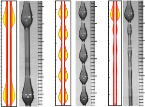
Figure 6. Comparison between the Navier–Stokes equations and experimental observations (adapted from Kliakhandler et al. Reference Kliakhandler, Davis and Bankoff2001). The dependent parameters are (a)  $\epsilon =0.2915$, $\alpha =0.2551$, $La=0.1633$; (b) $\epsilon =0.233$, $\alpha =0.2856$, $La=0.1458$; (c) $\epsilon =0.178$, $\alpha =0.3262$, $La=0.1276$. (a,b) Steady exact travelling wave solutions; (c) obtained by an elaborated direct numerical simulation.
Flow regime ‘c’ is a time-periodic state, which was suggested to be compared with a relative periodic orbit rather than a travelling wave solution (Ding & Willis Reference Ding and Willis2019). Although Ding & Willis (Reference Ding and Willis2019) predicted the cyclic coalescence and breakup dynamical process in flow regime ‘c’, the mean flow rate of their solution does not match the experimental result and the mean wave speed of their relative periodic orbit is approximately  $30\,\%$ higher than experiment. Unfortunately, we failed to obtain a converged exact relative periodic solution of the Navier–Stokes equations. To obtain the time-periodic state that can be compared with the experiment, we should start the simulation with a specific initial condition. In fact, the solutions of the Navier–Stokes equations are not unique. For the given parameters of flow regime ‘c’, other types of solutions do exist, such as multi-hump steady travelling waves and relative periodic solutions with different numbers of small beads (Ding & Willis Reference Ding and Willis2019). Hence, in order to compare with experiment, we designed a numerical experiment using the relative periodic solution of Ding & Willis (Reference Ding and Willis2019) as initial condition (the flow rate is also averaged in a time period of the solution: $\bar {Q}=({1}/{T})\int ^T_0Q\,\textrm {d}t$). A time stepping study showed that the saturated solution is time-periodic (see figure 7), and a typical profile of the interface shows a structure remarkably similar to the experimental photo (see figure 6c). The cyclic process shows that the large droplet catches up with and consumes its front small beads, and small droplets are regenerated to the rear of the large droplet due to the Rayleigh–Plateau instability. In addition, since the time-marching method converges to the periodic state, it implies that the time-periodic solution is stable. Moreover, we computed the average wave speed $c$ of the time-periodic state and recorded the maximal wave height and found that the relative error with the experimental data is approximately $3\,\%$, showing that the result of the long-wave model has been significantly improved. Therefore, the present study suggests that, to predict the nonlinear dynamics in different flow regimes, one can keep the flow rate unchanged in the numerical simulation (this can be done by introducing a free time-dependent parameter in the momentum equation, such that the flow rate at each time step can be adjusted), and the flow rate should be fixed and controlled by a pump rather than maintaining the fluid depth in the reservoir in experiments. When the flow rate in the numerical study (either the Navier–Stokes equations or the reduced models) matches the flow rate in the experiment, the dynamics can be predicted correctly.

Figure 7. Spatial–temporal diagram of the interfacial thickness  $S$, which indicates that the flow state is time-periodic. The dependent parameters are $\epsilon =0.178$, $\alpha =0.3262$, $La=0.1276$, i.e. the same as flow regime ‘c’.
4. Conclusions
This paper has revisited the dynamics of a thick film coating a vertical fibre. The Navier–Stokes equations are solved using a domain mapping technique. A dynamical systems theory approach has been employed to find the exact travelling wave solutions, which were compared with experimental studies. We have shown that larger droplets move faster and the small capillary wave in front of the large droplet, appearing in the solution of long-wave models, can be eliminated in our solution of the Navier–Stokes equations. Our numerical results also demonstrated that the wave speed and height can be enhanced by the inertial effect but reduced by the streamwise diffusion effect.
A crucial observation by us was that the mean radius computed from the flow rate of a saturated state, which was chosen as the initial mean radius of the liquid film in previous studies, does not correspond to the true mean radius of the film at the initial state. We found that even a small change in the initial radius of the film can have a significant impact on the flow rates of the steady travelling wave solutions, which accounts for the poor predictions of the wave speeds in experiments. By doing a bisectional search of the initial thickness of the film, we obtained travelling wave solutions of the same flow rates as those in the experimental studies of Kliakhandler et al. (Reference Kliakhandler, Davis and Bankoff2001). Comparing with the experimental data obtained by Kliakhandler et al. (Reference Kliakhandler, Davis and Bankoff2001), the travelling wave solutions showed excellent agreements with experimental flow regimes ‘a’ and ‘b’. This suggests that, when predicting the dynamics of a flow regime using a reduced model, it is important to match the flow rate rather than the fluid volume between the predicted solution and experiment.
The time-periodic state, flow regime ‘c’, is compared with a snapshot from a series of time-stepping simulations, which also showed an excellent agreement with the experimental study. The discrepancy of the mean wave speed and maximal height between the numerical solution and the experimental data has been improved to  $3\,\%$. Interestingly, our numerical simulation also showed that the coalescence and breakup process between a large droplet and small beads is a cyclic and stable process.
Acknowledgements
This paper is dedicated to the 100th anniversary of G.K. Batchelor. Z.D. was inspired by the monograph Perspectives in Fluid Dynamics by Batchelor et al. and started his research on liquid film flows 10 years ago. R.L. is supported by the National Natural Science Foundation of China (grant no. 51766002) and the Guangxi Natural Science Foundation (no. 2018GXNSFAA281331). Z.D. was supported by an EPSRC grant optimization in fluid mechanics (EP/P000959/1) and Heilongjiang Touyan Innovative Program Team. Z.D. also acknowledges the enlightening discussions with Professor E.J. Hinch and the invitation for this study from Professor P. Linden. We acknowledge the many constructive comments of the three referees.
Declaration of interests
The authors report no conflict of interest.


 Open access