


1 Introduction
It is well known that the interior of the Earth (Dziewonski & Anderson Reference Dziewonski and Anderson1981) and its moon (Weber et al. Reference Weber, Lin, Garnero, Williams and Lognonné2011) consist, in large part, of a liquid layer consisting of a molten iron alloy. This scenario is also likely for other terrestrial planets. Movements in this electrically conducting fluid are assumed to be the source of planetary magnetic fields (Stevenson Reference Stevenson2003). However, the energy source of the flow is not entirely certain. While models considering thermal and chemical convection had many successes in explaining key features of Earth’s field, such as the frequent reversals and dominantly bipolar structures (Christensen & Wicht Reference Christensen, Wicht and Gerald2015), several studies from different fields of the geosciences have shed doubt on the assumption (Dwyer, Stevenson & Nimmo Reference Dwyer, Stevenson and Nimmo2011; Olson Reference Olson2013; Andrault et al. Reference Andrault, Monteux, Le Bars and Samuel2016; Fuller Reference Fuller2017). Mechanical driving mechanisms have been proposed as a viable alternative, especially the precession of the rotation axis, which has been explored in numerous studies.
A fluid in an uniformly rotating container would settle to move with the boundaries as a constant vorticity flow when no other forcings are present. Precession describes the slower rotation of the diurnal rotation axis around another axis orthogonal to the ecliptic. When precession acts on the fluid, it tries to keep its original motion due to inertia, but the forcing constantly changes its direction. Viscous and topographic torques exerted by the boundaries work to align the flow with the time-dependent rotation of the boundaries. The base precessional bulk flow with the velocity  $u$ in a sphere at position $r$ and time $t$ therefore consists of a fluid motion that is similar to the rotation of a rigid body with a fluid rotation axis $\unicode[STIX]{x1D74E}_{f}\boldsymbol{ : }\boldsymbol{u}(\boldsymbol{r},t)=\unicode[STIX]{x1D74E}_{f}(t)\times \boldsymbol{r}$. The best known theoretical determination of $\unicode[STIX]{x1D74E}_{f}$ was made by Busse (Reference Busse1968), who considered the advection of a viscous boundary layer into the non-viscous interior to derive an implicit equation for the fluid rotation. This result was reobtained by Noir et al. (Reference Noir, Cardin, Jault and Masson2003) with a torque balance approach, which was later generalized by Noir & Cébron (Reference Noir and Cébron2013) to derive a differential equation describing the behaviour of $\unicode[STIX]{x1D74E}_{f}$. As a general trend, the fluid rotation lags behind the rotation of the container, a behaviour that has been observed in both laboratory experiments and numerical studies, e.g. Vanyo & Dunn (Reference Vanyo and Dunn2000), Tilgner & Busse (Reference Tilgner and Busse2001), Ernst-Hullermann, Harder & Hansen (Reference Ernst-Hullermann, Harder and Hansen2013) and Noir et al. (Reference Noir, Cardin, Jault and Masson2003). Secondary flow structures and various viscous and inertial instabilities can develop in addition to this laminar flow, such as inertial modes, shear layers, parametric or triadic resonances and the development of turbulence. We refer to Le Bars (Reference Le Bars2016) for a recent review on the subject. Several studies have shown, with the help of direct numerical simulations, that a planetary dynamo driven by precession is possible (Tilgner Reference Tilgner2005; Ernst-Hullermann et al. Reference Ernst-Hullermann, Harder and Hansen2013; Lin et al. Reference Lin, Marti, Noir and Jackson2016; Cébron et al. Reference Cébron, Laguerre, Noir and Schaeffer2019).
As mentioned in the first paragraph, many studies consider buoyancy as the main agent behind core flows. A buoyancy driven flow in a rotating shell, near the onset of convection, is characterized by two-dimensional structures that are aligned with the axis of rotation. In addition to these small scale convective columns, larger scale zonal flows develop (Dormy et al. Reference Dormy, Soward, Jones, Jault and Cardin2004; Aurnou Reference Aurnou2007). It has been hypothesized by Cheng et al. (Reference Cheng, Stellmach, Ribeiro, Grannan, King and Aurnou2015) that these structures are not stable at parameters relevant for planetary cores. Of special interest for the study of thermal convection is the amount of heat that can be transported in addition to the basic conductive profile. Scaling laws connect the heat flux to the thermal forcing and other parameters, where different scalings characterize different flow regimes (Aurnou Reference Aurnou2007; King et al. Reference King, Soderlund, Christensen, Wicht and Aurnou2010). A great advantage of such scalings is that they can be extrapolated to regimes that are (currently) unreachable by either laboratory or numerical experiments. We refer to the recent review by Plumley & Julien (Reference Plumley and Julien2019) for an overview on this subject with a focus on plane layer convection.
In this work, we combine a buoyancy forcing with a precessing rotation of the boundaries. A similar model was employed by Wei & Tilgner (Reference Wei and Tilgner2013), who considered a fixed, uniform background stratification in a spherical shell with a small stress-free inner core. They found that a stable stratification suppresses possible precessional instabilities, whereas an unstable stratification can lead to both stabilization and destabilization, depending on the parameters. This approach was later extended to the hydromagnetic case in Wei (Reference Wei2016), where it was shown that dynamos with a combined forcing are possible even when one forcing by itself leads to a failed dynamo. Here, we consider a non-uniform temperature stratification that is imposed by the temperature boundary conditions and we neglect the magnetic field. Our simulations have a larger inner core with no-slip boundaries. Most importantly, we look at flows in spheroidal shells, were theoretical models (Busse Reference Busse1968; Noir & Cébron Reference Noir and Cébron2013; Cébron Reference Cébron2015) have shown that the assumption of a linear, rigid-rotation-like bulk flow leads to multiple stable solutions at certain parameters, particularly low Ekman numbers or strong deformation of the boundary. This behaviour has been recreated in laboratory (Malkus Reference Malkus1968) and numerical experiments (Lorenzani & Tilgner Reference Lorenzani and Tilgner2003; Goepfert & Tilgner Reference Goepfert and Tilgner2016; Vormann & Hansen Reference Vormann and Hansen2018). We conduct a range of numerical simulations at a moderate Ekman number  $Ek=10^{-4}$ and show that this bistable behaviour persists when a temperature field is present. A jump to the second stable solution can not only be realized through a hysteresis, as for the purely mechanical forcing (Vormann & Hansen Reference Vormann and Hansen2018), but also by the influence of thermal convection. Further, we show which of the two flow types described above dominates dependent on the parameters and point out how they can be distinguished by decomposing the flow field into symmetric and asymmetric components.
We start by introducing the mathematical model of a precessing, fluid-filled spheroid in § 2, where some space is dedicated to concisely discussing the direction of gravity in a spheroidal shell. In § 3, we summarize the torque balance model by Noir & Cébron (Reference Noir and Cébron2013) that will be used for comparison to our numerical experiments. The results section is in two parts, where we first discuss the case of a varying precessional forcing at a constant Rayleigh number (§ 5.1) and then a smaller set of simulations where the Rayleigh number was increased at a constant precession rate (§ 5.2). The final § 6 summarizes and contextualizes the results.
2 Mathematical model of a fluid filled spheroid
Our model consists of a spherical or oblate spheroidal shell with outer radius  $r_{o}$ and inner radius $r_{i}$ in the horizontal plane. In Cartesian coordinates, the boundaries are defined by
 $$\begin{eqnarray}x^{2}+y^{2}+\frac{z^{2}}{(c/a)^{2}}=r_{o}\quad \text{and}\quad x^{2}+y^{2}+\frac{z^{2}}{(c/a)^{2}}=r_{i},\end{eqnarray}$$
 where  $a$ and $c$ are the horizontal major and vertical minor axes ( $c/a\leqslant 1$). The shell rotates with the frequency $\unicode[STIX]{x1D6FA}_{d}$ around the unit vector $\hat{\boldsymbol{z}}$ parallel to the minor axis and precesses with $\unicode[STIX]{x1D6FA}_{p}$ around another axis $\hat{\boldsymbol{k}}_{p}$ that forms an angle $\unicode[STIX]{x1D6FC}$ with $\hat{\boldsymbol{z}}$. We search for the velocity $\boldsymbol{u}=(u,v,w)$, pressure $p$ and temperature $T$ of a fluid that is described by the Boussinesq approximation, where density variations are only retained for the buoyancy term and depend linearly on the temperature difference. In a rotating reference frame where the boundaries are at rest (mantle frame), the relevant equations are the Navier–Stokes equation
 $$\begin{eqnarray}\frac{\unicode[STIX]{x2202}\boldsymbol{u}}{\unicode[STIX]{x2202}t}+\boldsymbol{u}\boldsymbol{\cdot }\unicode[STIX]{x1D735}\boldsymbol{u}=-\unicode[STIX]{x1D735}p+Ek\unicode[STIX]{x1D6FB}^{2}\boldsymbol{u}-2(\hat{\boldsymbol{z}}+\unicode[STIX]{x1D734}_{p})\times \boldsymbol{u}-(\unicode[STIX]{x1D734}_{p}\times \hat{\boldsymbol{z}})\times \boldsymbol{r}+RaT\boldsymbol{g},\end{eqnarray}$$
the incompressibility condition
 $$\begin{eqnarray}\unicode[STIX]{x1D735}\boldsymbol{\cdot }\boldsymbol{u}=0,\end{eqnarray}$$
and the heat equation
 $$\begin{eqnarray}\frac{\unicode[STIX]{x2202}T}{\unicode[STIX]{x2202}t}+\boldsymbol{u}\boldsymbol{\cdot }\unicode[STIX]{x1D735}T=\frac{Ek}{Pr}\unicode[STIX]{x1D6FB}^{2}T.\end{eqnarray}$$
In (2.2), the fourth term on the right-hand side, the Poincaré acceleration, includes the time-dependent precession axis
 $$\begin{eqnarray}\unicode[STIX]{x1D734}_{p}=Po\hat{\boldsymbol{k}}_{p}=Po\left(\begin{array}{@{}cc@{}}\phantom{+} & \sin \unicode[STIX]{x1D6FC}\cos t\\ - & \sin \unicode[STIX]{x1D6FC}\sin t\\ & \cos \unicode[STIX]{x1D6FC}\end{array}\right).\end{eqnarray}$$
 The equations have been non-dimensionalized with the diurnal rotation period  $\unicode[STIX]{x1D6FA}_{d}^{-1}$, the distance between the outer and inner core boundary $d=r_{o}-r_{i}$ and the temperature difference between inner and outer boundary $\unicode[STIX]{x0394}T=T_{i}-T_{o}$. With this scaling, the problem is governed by the Ekman number $Ek=\unicode[STIX]{x1D708}/(d^{2}\unicode[STIX]{x1D6FA}_{d})$, giving the ratio of viscous to rotational forces, the Poincaré number $Po=\unicode[STIX]{x1D6FA}_{p}/\unicode[STIX]{x1D6FA}_{d}$, which controls the relative strength of precession, the non-diffusive rotational Rayleigh number $Ra=\unicode[STIX]{x1D6FE}g_{0}\unicode[STIX]{x0394}T/(\unicode[STIX]{x1D6FA}_{d}^{2}r_{o})$ (with the expansivity $\unicode[STIX]{x1D6FE}$ and gravitation $g_{0}$ at $r_{o}$), controlling the strength of buoyancy and the Prandtl number $Pr=\unicode[STIX]{x1D708}/\unicode[STIX]{x1D705}$, which gives the ratio of viscosity $\unicode[STIX]{x1D708}$ to thermal diffusivity $\unicode[STIX]{x1D705}$. A negative $Po<0$ denotes retrograde precession, which is the case relevant for planets. The Rayleigh number can also be interpreted as the squared free-fall convective Rossby number, calculated from the ratio of a rotational to a free-fall time scale (Julien et al. Reference Julien, Legg, McWilliams and Werne1996). We use no-slip boundary conditions ( $\boldsymbol{u}=0$) for the velocity field and set the temperature to $T_{i}=1$ at the inner and $T_{o}=0$ at the outer boundary of the shell. Internal heat sources are not considered.
For the case of a spherical shell, the non-dimensional gravity vector in (2.2) is proportional to the radius:  $\boldsymbol{g}=\boldsymbol{r}$. Due to the broken symmetry, the formulation is more involved in a spheroidal shell. For simplicity, we assume that the inner part of the shell has the same density as the fluid filled volume. We then use the derivation by Hvoždara & Kohút (Reference Hvoždara and Kohút2012), where the gravity field on the inside of an oblate spheroidal body is calculated using fundamental solutions of the Laplace and Poisson equations in oblate spheroidal coordinates. These coordinates $(\unicode[STIX]{x1D702},\unicode[STIX]{x1D703},\unicode[STIX]{x1D719})$ are connected to Cartesian coordinates $(x,y,z)$ via
 $$\begin{eqnarray}\displaystyle & \displaystyle x=f\cosh \unicode[STIX]{x1D702}\sin \unicode[STIX]{x1D703}\cos \unicode[STIX]{x1D719}, & \displaystyle\end{eqnarray}$$
 $$\begin{eqnarray}\displaystyle & \displaystyle y=f\cosh \unicode[STIX]{x1D702}\sin \unicode[STIX]{x1D703}\sin \unicode[STIX]{x1D719}, & \displaystyle\end{eqnarray}$$
 $$\begin{eqnarray}\displaystyle & \displaystyle z=f\cosh \unicode[STIX]{x1D702}\cos \unicode[STIX]{x1D703}, & \displaystyle\end{eqnarray}$$
 with the geometry parameter  $f=\sqrt{a^{2}-c^{2}}$. The solution also requires Lame’s coefficient $h_{\unicode[STIX]{x1D702}}=h_{\unicode[STIX]{x1D703}}=f\sqrt{\cosh ^{2}\unicode[STIX]{x1D702}-\sin ^{2}\unicode[STIX]{x1D703}}$, the functions
 $$\begin{eqnarray}\displaystyle & \displaystyle q_{2}(t)=\frac{1}{2}\left((3t^{2}+1)\arctan \left(\frac{1}{t}\right)-3t\right) & \displaystyle\end{eqnarray}$$
 $$\begin{eqnarray}\displaystyle & \displaystyle \frac{\text{d}q_{2}}{\text{d}t}=q_{2}^{\prime }(t)=3t\arctan \left(\frac{1}{t}\right)+\frac{-3t^{2}-1}{2t^{2}+2}-\frac{3}{2} & \displaystyle\end{eqnarray}$$
 $$\begin{eqnarray}\displaystyle & \displaystyle P_{2}(t)={\textstyle \frac{1}{2}}(3t^{2}-1) & \displaystyle\end{eqnarray}$$
and the multiplication constant
 $$\begin{eqnarray}E_{2}=-\cosh ^{2}\unicode[STIX]{x1D702}_{0}(\cosh ^{2}\unicode[STIX]{x1D702}_{0}q_{2}^{\prime }(\sinh \unicode[STIX]{x1D702}_{0})-2\sinh \unicode[STIX]{x1D702}_{0}q_{2}(\sinh \unicode[STIX]{x1D702}_{0})),\end{eqnarray}$$
 where  $\unicode[STIX]{x1D702}_{0}$ is the constant value of $\unicode[STIX]{x1D702}$ on the outer boundary. With the gravitational constant $G$ and density $\unicode[STIX]{x1D70C}_{0}$, the dimensional solution for the inside of the shell in spheroidal coordinates in a two-dimensional (2-D) plane ( $g_{\unicode[STIX]{x1D719}}=0$) is then
 $$\begin{eqnarray}\displaystyle & \displaystyle g_{\unicode[STIX]{x1D702}}=-\frac{2\unicode[STIX]{x03C0}G\unicode[STIX]{x1D70C}_{0}\,f^{2}}{h_{\unicode[STIX]{x1D702}}}\cosh \unicode[STIX]{x1D702}\sinh \unicode[STIX]{x1D702}(\sin ^{2}\unicode[STIX]{x1D703}+E_{2}P_{2}(\cos \unicode[STIX]{x1D703})), & \displaystyle\end{eqnarray}$$
 $$\begin{eqnarray}\displaystyle & \displaystyle g_{\unicode[STIX]{x1D703}}=-\frac{2\unicode[STIX]{x03C0}G\unicode[STIX]{x1D70C}_{0}\,f^{2}}{h_{\unicode[STIX]{x1D703}}}\cos \unicode[STIX]{x1D703}\sin \unicode[STIX]{x1D703}\left(\cosh ^{2}\unicode[STIX]{x1D702}+\frac{1}{2}E_{2}(3\sinh ^{2}\unicode[STIX]{x1D702}+1)\right), & \displaystyle\end{eqnarray}$$
 which can be transferred to Cartesian coordinates in the  $xz$ plane via
 $$\begin{eqnarray}\displaystyle & \displaystyle g_{x}=(g_{\unicode[STIX]{x1D702}}\sinh \unicode[STIX]{x1D702}\sin \unicode[STIX]{x1D703}+g_{\unicode[STIX]{x1D703}}\cosh \unicode[STIX]{x1D702}\cos \unicode[STIX]{x1D703})(\cosh ^{2}\unicode[STIX]{x1D702}-\sin ^{2}\unicode[STIX]{x1D703})^{-1/2}, & \displaystyle\end{eqnarray}$$
 $$\begin{eqnarray}\displaystyle & \displaystyle g_{z}=(g_{\unicode[STIX]{x1D702}}\cosh \unicode[STIX]{x1D702}\cos \unicode[STIX]{x1D703}-g_{\unicode[STIX]{x1D703}}\sinh \unicode[STIX]{x1D702}\sin \unicode[STIX]{x1D703})(\cosh ^{2}\unicode[STIX]{x1D702}-\sin ^{2}\unicode[STIX]{x1D703})^{-1/2}\operatorname{sgn}(z). & \displaystyle\end{eqnarray}$$
 For positions outside the 2-D plane ( $g_{y}\neq 0$), the solution can be obtained by vector rotation around $\hat{\boldsymbol{z}}$, since the gravity field is symmetrical. For easier comparison to the spherical case, we normalize (and non-dimensionalize) the spheroidal gravity field so that both cases have the same value at the outer boundary in the horizontal plane ( $\sqrt{x^{2}+y^{2}}=r_{o}$, $z=0$). Since the base gravity enters into $Ra$, we should remember that the values are not directly comparable. Figure 1 shows an example of the resulting field in a 2-D plane for a strong flattening of $c/a=0.6$. The streamlines show that gravity is not directed directly at the centre of the mass distribution (at $(x,y,z)=(0,0,0)$). Instead, the tangential streamlines exhibit a slightly curved path. When looking at the magnitude of the non-dimensional gravity field, we observe that the field is strongest at the north and south poles of the spheroid, were the distance to the centre of mass is smaller than at the boundary in the horizontal plane. Additionally, contour lines of gravity are not parallel to the inner or outer boundary of the volume. These differences from the spherical case become less significant as $c/a$ moves closer to 1.
Of course, in a real planet, the shape is influenced by pressure, rotation and gravity, which is a complex problem (Tricarico Reference Tricarico2014). Our simplified model can be interpreted as a planetary body which shape was frozen in during an initial period of fast rotation and now has a rigid inner core and mantle. Studies of the early Earth suggest rotation rates up to ten times as high as those of today (Agnor, Canup & Levison Reference Agnor, Canup and Levison1999; Ćuk & Stewart Reference Ćuk and Stewart2012). For the case of strong rotation (low  $Ek$) one may also consider the inclusion of centrifugal effects, which we do not attempt here. We mainly consider a strong deformation of $c/a=0.8$ to reach a parameter region with possible bistability at acceptable computational cost – at smaller deformations, a much lower $Ek$ would be required.

Figure 1. Field lines (a) and contour lines (b) of the gravity field in a spheroidal shell with  $c/a=0.6$, in the $xz$ plane. Grey lines indicate the inner and outer boundary.
3 Dynamical model of the fluid rotation axis
In a purely precession driven flow ( $Ra=0$ in (2.2)), the main component of the flow outside of viscous boundary layers is often described as a linear rigid rotation around a fluid rotation axis $\unicode[STIX]{x1D74E}_{f}=(\unicode[STIX]{x1D714}_{x},\unicode[STIX]{x1D714}_{y},\unicode[STIX]{x1D714}_{z})$: $\boldsymbol{u}(\boldsymbol{r},t)=\unicode[STIX]{x1D74E}_{f}(t)\times \boldsymbol{r}$. Busse (Reference Busse1968) derived an implicit equation for the components of $\unicode[STIX]{x1D74E}_{f}$ based on the asymptotic advection of a viscous boundary layer flow to the non-viscous interior. Later, Noir et al. (Reference Noir, Cardin, Jault and Masson2003) derived the same result starting from a torque balance formulation of the Navier–Stokes equation. Both approaches assumed a time-independent, linearized equation ( $\unicode[STIX]{x2202}\boldsymbol{u}/\unicode[STIX]{x2202}t+\boldsymbol{u}\boldsymbol{\cdot }\unicode[STIX]{x1D735}\boldsymbol{u}=0$) and only considered the equatorial component of the viscous torque acting in the boundary layer, leading to a spin over mode. In their appendix A, Noir & Cébron (Reference Noir and Cébron2013) present an extended model that does not restrict the time dependency of the flow and allows for a spin up or spin down of the fluid from axial differential rotation. We use this model as a point of comparison for our numerical simulations and therefore concisely repeat the result. In a precessing frame of reference, where the precession axis $\unicode[STIX]{x1D734}_{p}=(\unicode[STIX]{x1D6FA}_{x},0,\unicode[STIX]{x1D6FA}_{z})=Po(\sin \unicode[STIX]{x1D6FC},0,\cos \unicode[STIX]{x1D6FC})$ is at rest, their dynamical model reads
 $$\begin{eqnarray}\frac{\unicode[STIX]{x2202}\unicode[STIX]{x1D74E}_{f}}{\unicode[STIX]{x2202}t}=\left(\begin{array}{@{}c@{}}\unicode[STIX]{x1D714}_{y}\unicode[STIX]{x1D6FA}_{z}\\ \unicode[STIX]{x1D714}_{z}\unicode[STIX]{x1D6FA}_{x}-\unicode[STIX]{x1D714}_{z}\unicode[STIX]{x1D6FA}_{z}\\ -\unicode[STIX]{x1D714}_{y}\unicode[STIX]{x1D6FA}_{x}\end{array}\right)+\frac{\displaystyle \left(\frac{c}{a}\right)^{2}-1}{\displaystyle \left(\frac{c}{a}\right)^{2}+1}\left(\begin{array}{@{}c@{}}-\unicode[STIX]{x1D714}_{y}\unicode[STIX]{x1D6FA}_{z}-\unicode[STIX]{x1D714}_{z}\unicode[STIX]{x1D714}_{y}\\ \phantom{-}\unicode[STIX]{x1D714}_{x}\unicode[STIX]{x1D6FA}_{z}+\unicode[STIX]{x1D714}_{x}\unicode[STIX]{x1D714}_{z}\\ -\unicode[STIX]{x1D714}_{y}\unicode[STIX]{x1D6FA}_{x}\end{array}\right)+{\mathcal{L}}\unicode[STIX]{x1D6E4}_{\unicode[STIX]{x1D708}}.\end{eqnarray}$$
The generalized viscous torque is
 $$\begin{eqnarray}{\mathcal{L}}\unicode[STIX]{x1D6E4}_{\unicode[STIX]{x1D708}}=\sqrt{Ek|\unicode[STIX]{x1D74E}_{f}|}\left[\frac{\unicode[STIX]{x1D706}_{so}^{r}}{\unicode[STIX]{x1D74E}_{f}^{2}}\left(\begin{array}{@{}c@{}}\unicode[STIX]{x1D714}_{x}\unicode[STIX]{x1D714}_{z}\\ \unicode[STIX]{x1D714}_{y}\unicode[STIX]{x1D714}_{z}\\ \unicode[STIX]{x1D714}_{z}^{2}-\unicode[STIX]{x1D74E}_{f}^{2}\end{array}\right)+\frac{\unicode[STIX]{x1D706}_{so}^{i}}{|\unicode[STIX]{x1D74E}|}\left(\begin{array}{@{}c@{}}\unicode[STIX]{x1D714}_{y}\\ -\unicode[STIX]{x1D714}_{x}\\ 0\end{array}\right)+\unicode[STIX]{x1D706}_{sup}\frac{\unicode[STIX]{x1D74E}_{f}^{2}-\unicode[STIX]{x1D714}_{z}}{\unicode[STIX]{x1D74E}_{f}^{2}}\left(\begin{array}{@{}c@{}}\unicode[STIX]{x1D714}_{x}\\ \unicode[STIX]{x1D714}_{y}\\ \unicode[STIX]{x1D714}_{z}\end{array}\right)\right],\end{eqnarray}$$
with the spin up decay factor (derived from the calculation of Greenspan & Howard (Reference Greenspan and Howard1963) for an axisymmetric container)
 $$\begin{eqnarray}\unicode[STIX]{x1D706}_{sup}=\frac{\sqrt{\unicode[STIX]{x03C0}^{3}/2}}{c\unicode[STIX]{x1D6E4}(0.75)^{2}}F(-0.25,0.5;0.75;1-c^{2}).\end{eqnarray}$$
 Here,  $\unicode[STIX]{x1D6E4}(z)$ is the Eulerian gamma function and $F(a,b;c;z)$ the hypergeometric series (Abramowitz & Stegun Reference Abramowitz and Stegun1972). For the spin over decay factors $\unicode[STIX]{x1D706}_{so}^{r}$ and $\unicode[STIX]{x1D706}_{so}^{i}$, we use the result from Zhang, Liao & Earnshaw (Reference Zhang, Liao and Earnshaw2004) and correct it for the presence of an inner core by multiplying with $h_{ic}(r_{i}/r_{o})=(1+(r_{i}/r_{o})^{4})(1-(r_{i}/r_{o}))/(1-(r_{i}/r_{o})^{5})$ (Hollerbach & Kerswell Reference Hollerbach and Kerswell1995) leading to
 $$\begin{eqnarray}\displaystyle & \displaystyle \unicode[STIX]{x1D706}_{so}^{r}=h_{ic}\left(\frac{r_{i}}{r_{o}}\right)\left(-2.62047-0.42634\left(1-\frac{c^{2}}{a^{2}}\right)\right), & \displaystyle\end{eqnarray}$$
 $$\begin{eqnarray}\displaystyle & \displaystyle \unicode[STIX]{x1D706}_{so}^{i}=h_{ic}\left(\frac{r_{i}}{r_{o}}\right)\left(\phantom{-}0.25846+0.76633\left(1-\frac{c^{2}}{a^{2}}\right)\right). & \displaystyle\end{eqnarray}$$
 The classical model by Busse (Reference Busse1968) as well as the dynamical model (3.1) by Noir & Cébron (Reference Noir and Cébron2013) allow multiple solutions for some parameter combinations, especially at low  $Ek$ or smaller $c/a$. This behaviour was further examined by Cébron (Reference Cébron2015), who gave approximate formulations for the range of parameters with several stable solutions. For the purpose of our study, we look for solutions to (3.1) by numerically searching for fixed points: starting with a fluid resting in the mantle frame of reference ( $\unicode[STIX]{x1D74E}_{f}=(0,0,1)$ in the precessing frame) at $Po=0$, we integrate the equations forward in time with a Runge–Kutta fourth-order time stepping scheme until a constant solution is reached. This solution is then used as a starting condition for the next larger value of $|Po|$, up to a maximum value. In order to find parameter combinations with multiple solutions, $|Po|$ is then again gradually decreased while taking the final $\unicode[STIX]{x1D74E}_{f}$ as the starting condition for the next smaller $|Po|$. For comparison to the results from the full numerical simulations, we do not consider the three components of $\unicode[STIX]{x1D74E}_{f}$ separately but instead look at the angular kinetic energy density in the mantle frame resulting from the rotation of the fluid about $\unicode[STIX]{x1D74E}_{f}$:
 $$\begin{eqnarray}E_{kin}^{N}={\textstyle \frac{1}{2}}(\unicode[STIX]{x1D74E}_{f}-\hat{\boldsymbol{z}})^{2}.\end{eqnarray}$$
 The substraction of  $\hat{\boldsymbol{z}}$ corrects for the rotation of the boundaries in the precessing frame of reference. This formulation ignores contributions from viscous boundary layers of an approximate thickness $1.4\sqrt{Ek}$ (Lorenzani & Tilgner Reference Lorenzani and Tilgner2001). In our numerical simulations, the total kinetic energy in the boundary layers is only approximately $1\,\%$ of the energy in the fluid bulk for all studied cases, leading us to neglect this inaccuracy.
4 Numerical method
We perform the direct numerical simulations with the spectral element code Nek5000 developed at Argonne National Laboratory (nek5000.mcs.anl.gov), in which the variables are represented in a weak formulation by high-order Lagrange polynomials defined on the Gauss–Lobatto–Legendre points in each element of a grid. The method combines high accuracy with geometric flexibility and very good parallel scaling capabilities and has been used for fluid mechanics problems both with mechanical forcings (Favier et al. Reference Favier, Grannan, Bars and Aurnou2015; Lemasquerier et al. Reference Lemasquerier, Grannan, Vidal, Cébron, Favier, Le Bars and Aurnou2017; Reddy, Favier & Bars Reference Reddy, Favier and Bars2018; Vormann & Hansen Reference Vormann and Hansen2018) and convection (Scheel & Schumacher Reference Scheel and Schumacher2014, Reference Scheel and Schumacher2016). The equations are integrated forward in time with a third-order accurate backward differentiation formula. A splitting method is used, where the viscous and pressure steps are handled as sub-problems with a Jacobi preconditioned conjugate gradient solver and an additive overlapping Schwarz method. We refer to Fischer (Reference Fischer1997), Deville, Fischer & Mund (Reference Deville, Fischer and Mund2002), Fischer & Lottes (Reference Fischer, Lottes and Barth2005) and Karniadakis & Sherwin (Reference Karniadakis and Sherwin2013) for details on the method.
The equations are solved on a cubed spheroidal grid as in Vormann & Hansen (Reference Vormann and Hansen2018). We project a Cartesian grid with points  $(\tilde{x}_{i},{\tilde{y}}_{i},\tilde{z}_{i})$ from each surface of a cube in the radial direction $\hat{\boldsymbol{r}}$ onto a spherical shell. The corner points of the spectral elements are placed at $(x_{ij},y_{ij},z_{ij})=r_{j}\hat{\boldsymbol{r}}_{i}$, where $r_{j}$ is a list of positions between $r_{i}$ and $r_{o}$ placed according to the Gauss–Legendre–Lobatto distribution, refining the grid in the radial direction at the outer and inner boundaries to better resolve viscous boundary layers. The resulting grid is then compressed in the $z$-direction by a factor $c/a$ to create a spheroid. The simulations reported here use a grid with $6144$ elements and polynomial orders $6$–
$6$– $12$.
$12$.
5 Results from direct numerical simulations
As mentioned in the introduction, this section on the results of our numerical experiments is split into two parts. All simulations have  $Ek=10^{-4}$, a relative inner core size of $0.35$ and a precession angle $\unicode[STIX]{x1D6FC}=23.5^{\circ }$. We first discuss simulations in different geometries ( $c/a=1$, $0.96$ and $0.8$) at fixed Rayleigh numbers $Ra=0.1$ and $Ra=1$ (§ 5.1). For $c/a=0.96$, we also used a computationally more demanding $Ra=10$. In a spherical shell, $Ra=0.1$ is approximately nine times overcritical, which is probably similar for a spheroidal shell. We started with the non-precessing case ( $Po=0$) of rotating convection and then gradually increased $|Po|$ at constant $Ra$. In the second set of experiments (§ 5.2), we considered a spheroidal shell with $c/a=0.8$ at a constant $Po=-0.075$ and, starting from a purely precessing flow ( $Ra=0$), increased the thermal forcing stepwise up to $Ra=5$. For all simulations, we examined retrograde precession with $Po<0$.
The important diagnostic parameters we will present are the kinetic energy density
 $$\begin{eqnarray}E_{kin}=\frac{1}{2V}\iiint _{V}\boldsymbol{u}^{2}\,\text{d}V\end{eqnarray}$$
and the Nusselt number
 $$\begin{eqnarray}Nu=\frac{\displaystyle \iint _{S_{o}}\boldsymbol{n}\boldsymbol{\cdot }\unicode[STIX]{x1D735}T\,\text{d}S_{o}}{\displaystyle \left.\iint _{S_{o}}\boldsymbol{n}\boldsymbol{\cdot }\unicode[STIX]{x1D735}T\,\text{d}S_{o}\right|_{Ra=0}^{Po=0}},\end{eqnarray}$$
 with the surface normal  $\boldsymbol{n}$ for the outer surface $S_{o}$. The value for the integral in the denominator of (5.2) for each geometry was obtained numerically in a simulation with $Ra=0$ and $Po=0$, since analytical solutions for spheroidal geometries are not available.
Studies of precession driven flows often decompose the velocity field into symmetric and antisymmetric components, since the basic precessional flow  $\boldsymbol{u}=\unicode[STIX]{x1D74E}_{f}\times \boldsymbol{r}$ is symmetric with respect to reflection at the origin of a Cartesian coordinate system $\boldsymbol{u}(\boldsymbol{r})=-\boldsymbol{u}(-\boldsymbol{r})$. The velocity field $\boldsymbol{u}$ is therefore separated into a symmetric component $\boldsymbol{u}_{s}=1/2(\boldsymbol{u}(\boldsymbol{r})-\boldsymbol{u}(-\boldsymbol{r}))$ and an antisymmetric component $\boldsymbol{u}_{a}=1/2(\boldsymbol{u}(\boldsymbol{r})+\boldsymbol{u}(-\boldsymbol{r}))$ from which corresponding symmetric and antisymmetric kinetic energies are derived
 $$\begin{eqnarray}E_{s}=\frac{1}{2V}\iiint _{V}\boldsymbol{u}_{s}^{2}\,\text{d}V\quad E_{a}=\frac{1}{2V}\iiint _{V}\boldsymbol{u}_{a}^{2}\,\text{d}V.\end{eqnarray}$$
An important diagnostic parameter is then the relative antisymmetric energy
 $$\begin{eqnarray}E_{rel}=\frac{E_{a}}{E_{a}+E_{s}}.\end{eqnarray}$$
 An increase in  $E_{rel}$ is often considered as a sign of instability of the base precessional flow. We ought to remember that the concept of antisymmetric energy is not as meaningful for a convection driven flow, where symmetry is not expected from the basic equations due to the buoyancy term. Still, we will see that the decomposition is useful to analyse our results.
For future reference, we have compiled most of the relevant data plotted in the figures in the results section in tables 1–7 and table 8, presented in the Appendix.

Figure 2. Value of  $E_{kin}$ in a spherical shell ( $c/a=1$) as a function of $Po<0$, compared to the solution of (3.1). Horizontal lines show the value of $E_{kin}$ for $Po=0$.

Figure 3. Value of  $E_{kin}$ in a spheroidal shell ( $c/a=0.96$) as a function of $Po<0$, compared to the solution of (3.1). Horizontal lines show the value of $E_{kin}$ for $Po=0$.

Figure 4. Value of  $E_{kin}$ in a spheroidal shell ( $c/a=0.8$) as a function of $Po<0$, compared to the solution of (3.1). Horizontal lines show the value of $E_{kin}$ for $Po=0$; ‘inc.’ and ‘dec.’ indicate whether $|Po|$ was increased or decreased from the starting field. Arrows indicate the use of starting conditions.

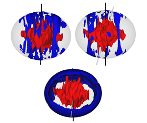
Figure 5. Exemplary visualizations of the velocity magnitude  $|\boldsymbol{u}|$ (blue) and temperature field $T$ for $c/a=0.8$, $Ra=0.1$ and three different Poincaré numbers $Po=0$ (a), $Po=-10^{-4}$ (b) and $Po=-0.1$ (c). The black line shows the axis of rotation, the white line the axis of precession.

Figure 6. Exemplary visualizations of the velocity magnitude  $|\boldsymbol{u}|$ (blue) and temperature field $T$ for $c/a=0.8$, $Ra=0.1$ for simulations with parameters in bistable regions. (a) $Ra=0.1$ and $Po=-0.1$ (decreased from $Po=-0.15$); (b) $Ra=1$ and $Po=-0.075$ (decreased from $Po=-0.1$). The black line shows the axis of rotation, the white line the axis of precession.

Figure 7. Time series of the kinetic energy density for  $Ra=0.1$ and $1$ at $c/a=0.8$ in the bistable region around $Po=-0.1$ to $-0.15$. Time has been reduced so that the plot starts at $t=0$.
5.1 Increasing the precessional forcing
The kinetic energy density (equation (5.1)) of the flow for  $Ek=10^{-4}$ remains relatively constant at the base value obtained for $Po=0$ over several orders of magnitude of $Po$(
$Po$( $O(10^{-7})$ to $O(10^{-3})$), as can be seen for the different geometries in figures 2–4. The plots show both the full range of $Po$ studied (figures on the left) and close ups for larger $Po$ (on the right). The base values for the non-precessing flow ( $Po=0$) are shown as horizontal lines in the figures, while black lines show solutions to (3.1). We do not show the full range of values for solutions of (3.1) to keep the figures compact. The kinetic energy density $E_{kin}$ is not the same for different geometries but decreases with $c/a$, i.e. the spherical case shows the largest absolute and relative kinetic energies (but remember that the definition of $Ra$ depends on $g_{0}$). Approximately at the value for $Po$ were the base kinetic energy becomes smaller than the rotational energy (3.6) predicted by (3.1) (which does not take buoyancy into account), at around $Po=-10^{-3}$ to $-10^{-2}$, the kinetic energy of the flow increases. Since this transition occurs at smaller precessional forcing for lower $Ra$, the kinetic energy increase happens for smaller $|Po|$ here. When we raise $|Po|$ further, we find the energy to be in good accordance with (3.6) for all values of $Ra$ and $c/a$, with a tendency to be slightly larger for a stronger thermal forcing. In figure 5, we see three exemplary visualizations of the velocity and temperature fields. For $Po=0$ and small $Po$, the flows are similar to typical patterns of rotating convection, with long structures in the velocity field parallel to the rotation axis. At an increased precessional forcing, a switch to a cylindrical, rigid-rotation-like flow structure occurs. For larger $Ra$, the situation is very similar, but smaller structures are formed.
The purely precession driven flow admits two stable solutions around  $Po=-0.1$ for $c/a=0.8$, depending on the starting field, as is predicted in (3.1), which does not include buoyancy effects. Our numerical experiments with a temperature field show a similar behaviour, as is evident in figure 4, where arrows illustrate the use of starting conditions. For the case of a low Rayleigh number $Ra=0.1$, a hysteresis occurs: the precessional forcing is first increased beyond the bistable region to $Po=-0.15$ and a new solution is realized when decreasing it again to $Po=-0.1$. When further decreasing the forcing, solutions on the lower branch are realized until we return to the solution with $E_{kin}$ similar to $Po=0$ beyond the transition point around $Po=-0.01$. For a larger $Ra=1$, the realization of multiple solutions happens without a hysteresis, as can be seen in the time series of the kinetic energy in figure 7. For the case of a larger thermal forcing, the flow directly switches to the branch of increased kinetic energy that is reached for lower $Ra$ only when coming from a larger precessional forcing, i.e. the bistability is not realized by the starting condition but by the additional buoyancy term. When further decreasing the precessional forcing, the behaviour is analogous to $Ra=0.1$, only the transition occurs earlier. Figure 6 shows two exemplary visualizations of flows in the bistable region, which are very similar in appearance to the figures discussed above.

Figure 8. Values of  $E_{rel}$ (a) and $E_{a}$ and $E_{s}$ (b) for $c/a=1$ as a function of $Po<0$.

Figure 9. Values of  $E_{rel}$ (a) and $E_{a}$ and $E_{s}$ (b) for $c/a=0.96$ as a function of $Po<0$.

Figure 10. Value of  $E_{rel}$ (a) and $E_{a}$ and $E_{s}$ (b) for $c/a=0.8$ as a function of $Po<0$; ‘inc.’ and ‘dec.’ indicate whether $|Po|$ was increased or decreased from the starting field.
The relative antisymmetric energy (equation (5.4)) is shown as a function of the Poincaré number  $Po$ in figures 8–10 (left figures). As for the full kinetic energy, the value of $E_{rel}$ remains nearly constant at approximately $0.5$ over a wide range of $Po$ up to the transition between the base thermal and rigid rotation solutions for the kinetic energy, as we would expect for a flow with no inherent symmetry. When reaching the Poincaré number beyond which $E_{kin}$ is predicted by the solution to the dynamic system (3.1), we observe a sharp drop in $E_{rel}$ by approximately two to three orders of magnitude. For lower $Ra$, the decrease in $E_{rel}$ is more pronounced: we can roughly estimate from the limited data that the decrease is inversely proportional to $Ra$. For example, in the spheroidal shell with $c/a=0.96$, $E_{rel}$ reduces to approximately $2\times 10^{-1}$ at $Ra=10$, to $3\times 10^{-2}$ at $Ra=1$ and goes down to $E_{rel}=3\times 10^{-3}$ at $Ra=0.1$. The plots to the right in figures 8–10 further explore the behaviour of the two flow components: there, $E_{a}$ and $E_{s}$ are shown separately as functions of $Po$. The antisymmetric energy is larger for larger $Ra$ and remains approximately independent of $Po$, only a slight increase for larger precessional forcing is observed. The exception here is $E_{a}$ for the hysteresis loop at $Ra=0.1$, were it increases by approximately one order of magnitude and becomes nearly as large as for $Ra=1$. The symmetric part $E_{s}$ of the energy increases by several orders of magnitude for all values of $Ra$ when reaching the value of $Po$ for which the overall kinetic energy $E_{kin}$ also increases. For large precessional forcings, $E_{s}$ becomes nearly independent of the Rayleigh number, while the differences in $E_{a}$ remain. An increase in $Ra$ by one order of magnitude seems to produce the same increase in $E_{a}$, explaining the differences in $E_{rel}$.
Generally, the heat transfer represented by  $Nu$ is very similar between different geometries, as can be seen in figure 11. We observe that the heat flux is slightly lowered by the introduction of precession for $Ra=0.1$ and $1$, with a greater decrease for a larger $Ra=10$. A clear increase of $Nu$ above the base value is only observed for larger $|Po|$ at $c/a=0.8$ and $Ra=0.1$. There, $Nu$ stays at the higher value when the forcing is decreased again to investigate the hysteresis behaviour and then returns to its original value.

Figure 11. Value of  $Nu$ at the outer boundary as a function of $Po<0$ for different Rayleigh numbers $Ra$ and geometries: $c/a=1$ (a), $c/a=0.96$ (b) and $c/a=0.8$ (c). Horizontal lines show the value of $Nu$ for $Po=0$.
For further verification, one simulation ( $c/a=0.8$, $Ra=1$ and $Po=-0.025$) was integrated in time for $12\,000$ time units to exclude long-term effects that are not visible in the other simulations; $12\,000$ rotational time units are equal to $1.2$ time units based on thermal diffusion. In figure 12, we see time series of $E_{kin}$ and the Nusselt number $Nu$ (equation (5.2)) for this case. While we observe oscillations of approximately $\pm 10\,\%$ around the mean value, no long-term positive or negative trend is visible and no notable outliers occur. Note that in cases with a stronger precessional forcing, as in figure 7, the oscillations are much smaller after the initial transient.

Figure 12. Time series of  $Nu$ (a) and $E_{kin}$ (b), both normalized with their mean value, for $Ek=10^{-4}$, $Ra=1$ and $Po=-0.025$, running for approximately 12 000 time units.
5.2 Varying thermal forcing
In this section, we look at a set of numerical simulations were the Poincaré number was held constant at  $Po=-0.075$ ( $c/a=0.8$ and $Ek=10^{-4}$) and the Rayleigh number was gradually increased starting from a pure precessional flow at $Ra=0$ up to $Ra=5$. The value $Po=-0.075$ lies inside a bistable region, as was shown in the previous section. We started with a solution on the lower branch of $E_{kin}$, i.e. $|Po|$ was increased to reach the starting field. Note that, where possible, the figures also include data from simulations with $Po=0$ and the respective $Ra$ for comparison. We performed one additional experiment at $Ra=5$ and $Po=0$ as a comparison for the highest thermal forcing. Simulations with increasing $Ra$ at $Po=0$, where we searched for $Nu>1$, indicate a critical Rayleigh number of $Ra_{c}\approx 4.75\times 10^{-3}$. Compared to the non-precessing flow, our values for $Ra$ are therefore 5 to 1000 times overcritical. For comparison, the critical $Ra$ for $c/a=0.96$ and $c/a=1$ is approximately $5\times 10^{-3}$.
Figure 13 shows results for the kinetic energy density  $E_{kin}$ (5.1) and Nusselt number $Nu$ (5.2). The kinetic energy shows that the base value for $Ra=0$ is slightly below the value of $E_{kin}\approx 0.024$ for a solution of the dynamical model (3.1). When increasing $Ra$, the energy increases but stays close to this value. A fit to the data is relatively difficult due to the small range of values for $E_{kin}$. Up to the transitional Rayleigh number $Ra_{t}=Ek^{-7/4}Ek^{2}Pr^{-1}(1-r_{i}/r_{o})^{-1}\approx 0.15$ (King et al. Reference King, Soderlund, Christensen, Wicht and Aurnou2010), a quadratic function $E_{kin}=0.0381Ra^{2}+0.0187$ describes the data well, while a linear function $E_{kin}=0.0068Ra+0.0193$ fits for larger $Ra>Ra_{t}$. The energies for the same value of $Ra$ at $Po=0$ (see figure 4) are smaller by orders of magnitude for small $Ra$, approximately $6.5\times 10^{-3}$ ( $Ra=1$) and $2.5\times 10^{-4}$ ( $Ra=0.1$). For $Ra=5$, the kinetic energy for the precessing flow is approximately $28\,\%$ larger than for the non-precessing experiment. The Nusselt number also increases from a base value of $Nu=1.014$, starting with a steep increase that decreases as $Ra$ becomes larger. We have $Nu>1$ at $Ra=0$ since the precessing flow by itself transports a small amount of heat. Here, the fit is clearer than for $E_{kin}$. In the considered range of $Ra$,
$Ra$,  $Nu$ can be fitted by functions $Nu=58Ra^{6/5}-1.06$ for $Ra<Ra_{t}$ and $Nu=14.8Ra^{2/7}+1.1$ for $Ra>Ra_{t}$. We tried different exponents from the literature on (non-)rotating convection (Ahlers, Grossmann & Lohse Reference Ahlers, Grossmann and Lohse2009; Cheng et al. Reference Cheng, Stellmach, Ribeiro, Grannan, King and Aurnou2015; King et al. Reference King, Soderlund, Christensen, Wicht and Aurnou2010) and found that these two exponents and the transitional $Ra_{t}$ provide the best explanation of the data. Here, the data for $Po=0$ are very similar, as was already seen in figure 11, where we found $Nu$ to be nearly independent of $Po$.
$Po$.

Figure 13. Values of  $E_{kin}$ (a) and $Nu$ (b) of a flow at fixed $Po=-0.075$, $Ek=10^{-4}$ and $c/a=0.8$ with increasing $Ra$. The dotted horizontal lines show $E_{kin}=0.024$ from the dynamical model (3.1) and the base value $Nu=1.014$ for $Ra=0$, while the vertical line marks the transitional Rayleigh number $Ra_{t}\approx 0.15$. The figures also show fitted functions $E_{kin}=0.0381Ra^{2}+0.0187$, $E_{kin}=0.0068Ra+0.0193$, $Nu=58Ra^{6/5}-1.06$ and $Nu=14.8Ra^{2/7}+1.1$ (dashed and solid lines). $\times$ marks values for $Po=0$. For small $Ra$, the values for $E_{kin}$ are: $6.5\times 10^{-3}$ ( $Ra=1$) and $2.5\times 10^{-4}$ ( $Ra=0.1$). The exact best fit values for the fit of the exponents in (b) are $0.283\pm 0.004$ and $1.19\pm 0.01$.

Figure 14. Values of  $E_{rel}$ (a) and $E_{a}$ and $E_{s}$ (b) at fixed $Po=-0.075$, $Ek=10^{-4}$ and $c/a=0.8$ with increasing $Ra$;
$Ra$;  $\times$ and $+$ mark values for $Po=0$.

Figure 15. Components of the fluid rotation vector  $\unicode[STIX]{x1D74E}_{f}$ $=$ (
$=$ ( $\unicode[STIX]{x1D714}_{x}$ (a), $\unicode[STIX]{x1D714}_{y}$ (b), $\unicode[STIX]{x1D714}_{z}$ (c)) as a function of $Ra$. Dashed horizontal line: solution for $Ra=0$, dotted horizontal line: solution of (3.1).
Figure 14 shows how the symmetric and antisymmetric components of the flow behave as  $Ra$ is increased. The relative energy $E_{rel}$ changes by several orders of magnitude as $Ra$ rises, from $O(10^{-8})$ up to $O(10^{-1})$, with the largest increase when going from $Ra=0$ to $Ra=0.025$. The separate plots of $E_{a}$ and $E_{s}$ show that this change is mainly due to an increase in $E_{a}$. The value of $E_{s}$ shows a linear increase with $Ra$ that is very similar to the overall behaviour of $E_{kin}$ (figure 13), while the antisymmetric component $E_{a}$ increases exponentially fast, although it stays below $E_{s}$ in the considered range. A fit of a linear function to the $E_{s}$ data gives $E_{s}=0.0042Ra+0.020$, showing that the symmetric energy increases slower with $Ra$ than the overall energy. The comparison with non-precessing experiments show that, there, both components are smaller but approximately equal, reflecting the results for small precessional forcing shown in figures 8–10. We observe that the fluid rotation vector $\unicode[STIX]{x1D74E}_{f}$, estimated from the mean bulk vorticity $\unicode[STIX]{x1D74E}_{f}\approx 1/(2V)\iiint \unicode[STIX]{x1D735}\times \boldsymbol{u}\,\text{d}V$ outside of viscous boundary layers, remains approximately constant at $\unicode[STIX]{x1D74E}_{f}\approx (-0.13,-0.039,0.98)$, where the solution from the dynamical system (3.1) is $\unicode[STIX]{x1D74E}_{f}=(-0.21,-0.033,0.96)$. The value of $\unicode[STIX]{x1D74E}_{f}$ is shown as a function of $Ra$ in figure 15, where we see that it remains largely unchanged as $Ra$ increases. A minor trend is observable, where the magnitude of the vector components slightly increases at first and then decreases for the largest $Ra$. We further explore the behaviour of $\unicode[STIX]{x1D74E}_{f}$ with the four visualizations in figure 16. Just as in figure 5, they depict characteristic isosurfaces of the velocity magnitude and temperature. For $Ra=0$, the precession flow is dominant and only leads to a small deformation of the conductive temperature profile. As the Rayleigh number increases, smaller structures emerge, but the linear rotation clearly dominates for $Ra=0.1$ and $1$. At the largest $Ra=5$, the large roll structure is hardly visible on the small scales, though the measurements of $\unicode[STIX]{x1D74E}_{f}$ still indicate its presence.

Figure 16. Visualizations of flows with constant  $Po=-0.075$ and increasing $Ra=0$ (a), 0.1 (b), 1 (c) and 5 (d), with isosurfaces of the temperature $T$ (red) and velocity magnitude $|\boldsymbol{u}|$ for representative values. The straight lines are the axes of diurnal (black) and precessional (white) rotation.
6 Discussion
This study presented numerical experiments on convection in precessing spherical and spheroidal shells. We found that, at a constant Rayleigh number  $Ra$, the flow remains largely independent of the precession over a wide range of values for $Po$ and can be classified as rotating convection. A change occurs when the kinetic energy predicted by the dynamical system (3.1) by Noir & Cébron (Reference Noir and Cébron2013) becomes larger than the base energy for $Po=0$. After that, the flow can be described as precession dominated and is well described by the model (3.1), although a small influence of $Ra$ remains. The transition is accompanied by a strong increase in the symmetric component of the velocity field, which becomes independent of $Ra$, while the antisymmetric component remains approximately constant. As was shown in Lorenzani & Tilgner (Reference Lorenzani and Tilgner2001), the precessional forcing only drives the symmetric component of the flow, while buoyancy has no preference for either component. A convection dominated flow therefore results in $E_{rel}\approx 0.5$, while a precession dominated flow results in much smaller values. The bistability predicted by Noir & Cébron (Reference Noir and Cébron2013) is reproduced in our simulations, again for a strong deformation of $c/a=0.8$. Here, the resulting solution depended on the starting condition for a small thermal forcing $Ra=0.1$. This behaviour is very similar to the purely precession driven flows reported in Vormann & Hansen (Reference Vormann and Hansen2018). For an increased thermal forcing of $Ra=1$, the simulation switches to a different branch by itself, showing that an external influence can change a precessing flow in the bistable parameter range. We note that the values of $E_{rel}$ for the purely mechanically driven flow ( $Ra=0$) reported in Vormann & Hansen (Reference Vormann and Hansen2018) are several orders of magnitude smaller, even when the total kinetic energy is very similar. Here, and in the experiments discussed in the next paragraph, we only observe a minor influence of precession on the heat flux.
In the second numerical experiment with an increasing  $Ra$, it was found that both $E_{kin}$ and $Nu$ increase with $Ra$, with an approximately quadratic and linear dependence for $E_{kin}$ and a proportionality to $Ra^{6/5}$ and $Ra^{2/7}$ for $Nu$. Malkus (Reference Malkus1954) first proposed an exponent of $1/3$ for the non-rotating Rayleigh–Bénard system, while Shraiman & Siggia (Reference Shraiman and Siggia1990) gave an exponent of $2/7$ based on a study of the nesting of the thermal inside the viscous boundary layer. King et al. (Reference King, Soderlund, Christensen, Wicht and Aurnou2010) studied the heat transfer for dynamos in rotating shells with the help of direct numerical simulations and found scaling exponents of $6/5$ (rapidly rotating regime) and $2/7$ (weakly rotating regime), which validity regions are separated by a transitional Rayleigh number $Ra_{t}=Ek^{-7/4}Ek^{2}\Pr ^{-1}(1-r_{i}/r_{o})^{-1}$ (in our notation). A similar result was found for convection in a plane layer in King et al. (Reference King, Stellmach, Noir, Hansen and Aurnou2009). They argue that the transition between the two regimes occurs when the size of the thermal and viscous boundary layers are equal. We note that the scaling in the rapidly rotating system also depends on the critical Rayleigh number, which in turn depends on the Ekman number. Since we only studied $Ek=10^{-4}$, we cannot make any further comments on this. King, Stellmach & Aurnou (Reference King, Stellmach and Aurnou2012) argued that the scaling may not hold at more extreme $Ra$ and $Ek$. For both rotating and non-rotating convection in cylindrical containers (laboratory) and periodic Cartesian boxes (direct numerical simulations), Cheng et al. (Reference Cheng, Stellmach, Ribeiro, Grannan, King and Aurnou2015) found similar relations of $Nu\propto Ra^{0.322}$ and $Nu\propto Ra^{1.29}$. However, they studied a much wider range of $Ek$,
$Ek$,  $Ra$ and $Nu$ than our simulations and found other relations of the form $Nu\propto Ra^{\unicode[STIX]{x1D6FD}}$ between the Rayleigh number and the heat flux, for example a steep scaling regime of $Nu\propto Ra^{3.6}$. At $Ek=10^{-4}$, they also found a larger exponent of $1.7$, while the exponent $1.29$, which is closest to our findings, appears at $Ek=10^{-3}$. For large enough $Ra$, the scaling converges towards the non-rotating case with exponent $0.322$. We need to point out that a clear distinction between the exponents $2/7$ and $1/3$ for $Ra>Ra_{t}$ is not possible with our limited data, since the resulting fit is of similar quality for both cases. Still, it is encouraging to see that precessing convection seems to share basic features with rotating convection. Cheng et al. (Reference Cheng, Stellmach, Ribeiro, Grannan, King and Aurnou2015) hypothesize a relation of the change in heat transfer regimes to the breakdown of coherent columnar structures. We have seen in our experiments that strong precessional forcing can also lead to the breakdown of such structures. At the parameter combinations shared between both sets of experiments, $Po=-0.075$ and $Ra=1$ or $Ra=0.1$, the diagnostic parameters differ by less than $1\,\%$, which is well within the range of the fluctuations of the numerical solution. It is left to future studies to find out if a further increase in thermal forcing can trigger a switch to the branch of increased $E_{kin}$ for a precessional flow, as happened for $Po=-0.1$ and $Ra=1$ when increasing the precessional frequency, although it seems unlikely since the bistability is predicted by a model that ignores buoyancy. Since the transitional $Ra_{t}$ as given above is dependent on $Ek$, studies with varying $Ek$ and a measurement of the layer thickness are necessary to elucidate the heat transfer behaviour. Studies of rapidly rotating Rayleigh–Bénard convection at smaller $Ek$ have shown a dependence of the heat transfer exponent on $Ek$. For a stronger rotation, an increased heat transfer occurs (Julien et al. Reference Julien, Aurnou, Calkins, Knobloch, Marti, Stellmach and Vasil2016; Plumley et al. Reference Plumley, Julien, Marti and Stellmach2016; Cheng et al. Reference Cheng, Aurnou, Julien and Kunnen2018). Since our results are similar at a moderate $Ek$, we might expect respective results for a precessing spheroid when approaching planetary relevant values.

Figure 17. Value of  $E_{kin}$ for solutions of the model by Busse (Reference Busse1968) for the terrestrial planets and Earth’s moon as a function of the retrograde precessional forcing $Po<0$. The parameters are $c/a=299/300$ and $\unicode[STIX]{x1D708}=5\times 10^{-7}~\text{m}^{2}~\text{s}^{-1}$ (Jones Reference Jones and Schubert2015), while $Ek$,
$Ek$,  $\unicode[STIX]{x1D6FC}$ and $c/a$ vary as follows: Earth ( $\unicode[STIX]{x1D6FC}=23.44^{\circ }$, $Ek=8.4\times 10^{-15}$), Moon ( $\unicode[STIX]{x1D6FC}=6.7^{\circ }$, $Ek=3.3\times 10^{-11}$), Mercury ( $\unicode[STIX]{x1D6FC}=0.03^{\circ }$, $Ek=7.8\times 10^{-13}$), Venus ( $\unicode[STIX]{x1D6FC}=177.4^{\circ }$, $Ek=10^{-12}$) and Mars ( $\unicode[STIX]{x1D6FC}=25.19^{\circ }$, $Ek=1.4\times 10^{-14}$). The relative inner core sizes are $r_{i}/r_{0}=0.35$ for the Earth and $r_{i}/r_{0}=0.46$ for the Moon. We set $r_{i}/r_{0}=0$ for the other planets due to missing seismic data on the existence of an inner core. The shaded region shows an estimate of the kinetic energy density for flows in the Earth’s core based on estimated velocities for the core flow (Stefan, Dobrica & Demetrescu Reference Stefan, Dobrica and Demetrescu2017). Vertical lines show the values of $Po$ for the four planets and the Moon and circles mark the intersection with the associated model. The data on the planetary structures and rotation are compiled from Weber et al. (Reference Weber, Lin, Garnero, Williams and Lognonné2011), Rivoldini et al. (Reference Rivoldini, Van Hoolst, Verhoeven, Mocquet and Dehant2011), Aitta (Reference Aitta2012), Smith et al. (Reference Smith, Zuber, Phillips, Solomon, Hauck, Lemoine, Mazarico, Neumann, Peale and Margot2012) and Van Hoolst (Reference Van Hoolst and Gerald2015).
Cébron, Maubert & Le Bars (Reference Cébron, Maubert and Le Bars2010) also combined thermal and mechanical forcings in a numerical study of the tidal instability in an ellipsoidal shell. They focussed on the growth of the tidal instability and also measured the resulting heat flux. The results indicate a transitional Rayleigh number proportional to  $Ek^{-8/5}$, based on a competition between the heat transfer by the tidal instability and natural convection. Similar arguments might be made for the precessional flow, though this requires information on the heat flow generated by precessional instabilities.
The results of our simulations indicate that the modelled flow can be described as a competition between precession and convection, were established features of both flow types are present, such as the bistability of the precessing flow and the heat transport scaling of thermal convection. The dominance of either type of flow can be shown by studying the relative strengths of symmetric and antisymmetric components in the velocity field, were the symmetric component is well described by the model of precessing flow constructed by Noir & Cébron (Reference Noir and Cébron2013). When this component is dominant, the precession roll component of the flow overlays the convective columns.
7 Implications for planetary flows
For a real planet, we can assume that the precessional forcing slowly declines due to tidal friction. If  $|Po|$ decreases below a certain value, the kinetic energy of the precessional flow becomes smaller than the value for $E_{kin}$ of a purely thermal flow at the core’s $Ra$. At this point, we might expect the core flow to switch from a precessing to a convecting state and remain there as $|Po|$ decreases further. If bistable solutions are possible, this change might occur very suddenly as the flow ‘drops’ to a convective state at the boundary of the bistable region. Of course, if the kinetic energy of the precessional flow is always larger than the convective flow (i.e. if $Ra$ is too small), convective processes might not be very important at all. If, on the other hand, $Ra$ is large enough, the convective flow can completely overlay the precessional solution. However, smaller contributions of the opposing flow forcings are of course possible. Figure 17 shows the kinetic energy density derived from the model by Busse (Reference Busse1968) for representative planetary parameters from the literature and $c/a=299/300$ for varying retrograde precessional forcing (see the figure caption for details). We note that solutions for the dynamical system (3.1) at small $Ek\approx 10^{-15}$ for the full range of $Po$ are computationally expensive and have therefore been omitted. Tests for some selected values show that the results are similar enough for this approximate comparison (although we have observed that qualitative differences may occur at larger forcing). Horizontal lines show an approximate range for the kinetic energy density of the flow in Earth’s outer core. For this estimate, we use approximate velocities for the core flow of $17$ to $40~\text{km}~\text{a}^{-1}$, based on the values given for magnetic flux patches in Stefan et al. (Reference Stefan, Dobrica and Demetrescu2017). The kinetic energy predicted for the purely precessional flow for the Earth at $Po\approx -10^{-7}$ is clearly below the estimates for the core flow, which might indicate that the core is not in a state dominated by precession. But, as mentioned in the introduction, other studies point in the opposite direction, so that our simple ad hoc model can certainly not give a definitive answer. Lower estimates for the core’s Rossby number of $10^{-7}{-}10^{-6}$, as given in Aurnou (Reference Aurnou2007) and Christensen & Wicht (Reference Christensen, Wicht and Gerald2015), would actually place the prediction for the precessing flow above the flow energy for the core. We see that the Earth at $Po=-10^{-7}$ is not in a region of possible bistability, as are the other planets. Still, the possibility of multiple solutions cannot be easily refuted. The large relative precession rates at which the bistability occurs might be more likely to be realized in smaller satellites that are under the influence of a more massive planet, as for example $|Po|$ for the Moon is slightly above the bistability range, while it is clearly below for the planets.
8 Outlook
Further work on this topic could include the examination of other geometries (ellipsoids, different inner core shapes, differential rotation) and an expansion to more realistic parameters (lower  $Ek$ and $Pr$). Apart from the bistability of the precessing flow, the spheroidal shape is also of interest for the study of convection. To our knowledge, only Evonuk (Reference Evonuk2015) considered the effect of an ellipsoidal deformation on the patterns of convection in a 2-D equatorial plane. While we did not focus on this topic, our model of a 3-D spheroid can act as a starting point for further research. Also note that we did not determine the critical Rayleigh number for the onset of convection as a function of the geometry and precession rate, but always took clearly overcritical $Ra$.
$Ra$.
Acknowledgements
This work is supported by the ‘Deutsche Forschungsgemeinschaft’ DFG in the framework of the priority programme SPP 1488 ‘Planetary Magnetism’. The authors gratefully acknowledge the Gauss Centre for Supercomputing (GCS) for providing computing time through the John von Neumann Institute for Computing (NIC) on the GCS share of the supercomputer JUQUEEN at Jülich Supercomputing Centre (JSC). GCS is the alliance of the three national supercomputing centres HLRS (Universität Stuttgart), JSC (Forschungszentrum Jülich) and LRZ (Bayerische Akademie der Wissenschaften), funded by the German Federal Ministry of Education and Research (BMBF) and the German State Ministries for Research of Baden-Württemberg (MWK), Bayern (StMWFK) and Nordrhein-Westfalen (MIWF).
Declaration of interests
The authors report no conflict of interest.
Appendix
Table 1. Results from direct numerical simulations at  $Ek=10^{-4}$, $c/a=1$, $Ra=0.1$ and varying $Po$.
$Po$.

Table 2. Results from direct numerical simulations at  $Ek=10^{-4}$, $c/a=1$, $Ra=1$ and varying $Po$.
$Po$.

Table 3. Results from direct numerical simulations at  $Ek=10^{-4}$, $c/a=0.96$, $Ra=0.1$ and varying $Po$.
$Po$.

Table 4. Results from direct numerical simulations at  $Ek=10^{-4}$, $c/a=0.96$, $Ra=1$ and varying $Po$.
$Po$.

Table 5. Results from direct numerical simulations at  $Ek=10^{-4}$, $c/a=0.96$, $Ra=10$ and varying $Po$.
$Po$.

Table 6. Results from direct numerical simulations at  $Ek=10^{-4}$, $c/a=0.8$, $Ra=0.1$ and varying $Po$. Data below the empty line come from experiments where the precessional forcing was decreased.

Table 7. Results from direct numerical simulations at  $Ek=10^{-4}$, $c/a=0.8$, $Ra=1$ and varying $Po$. Data below the empty line come from experiments where the precessional forcing was decreased.

Table 8. Results from direct numerical simulations at  $Ek=10^{-4}$, $c/a=0.8$, $Po=-0.075$ and increasing $Ra$.
$Ra$.


 Open access