


1. Introduction
High-energy and repeated wave impacts on coastal cliffs cause hydraulic fractures and ultimately release large sections of rock to create clifftop boulders (Herterich, Cox & Dias Reference Herterich, Cox and Dias2018). By virtue of their creation, these clifftop boulders are then exposed to high-energy seas and may be transported by the action of the waves (Cox et al. Reference Cox, Zentner, Kirchner and Cook2012). Kennedy, Cox & Dias (Reference Kennedy, Cox and Dias2021) showed that many assumed tsunami-induced boulder movements are, more probably, storm-wave induced. Additionally, Cox et al. (Reference Cox, Jahn, Watkins and Cox2018) gave evidence for the movement of clifftop boulders as large as 620 t by storm waves on the Irish west coast during the winter of 2013–2014. Consequent laboratory studies at  $1\,{:}\,100$ scale used an irregular sea to observe multiple transport and imbrication modes of clifftop boulder groups, many of them displaced by breaking waves (Cox, O'Boyle & Cytrynbaum Reference Cox, O'Boyle and Cytrynbaum2019).
Breaking waves are characterised by an overturning crest, primarily initiated by reducing depth (shoaling) (Peregrine Reference Peregrine1983), superposition of dispersive wave spectrum components and the exchange of wave energy between frequency components (nonlinear focusing) (Banner & Peregrine Reference Banner and Peregrine1993). The wave-breaking process begins when fluid velocities at the free surface exceed  ${\approx }0.85c_p$, where $c_p$ is the crest velocity (Barthelemy et al. Reference Barthelemy, Banner, Peirson, Fedele, Allis and Dias2018). Throughout the breaking process, the wave crest drastically changes shape and entrains air (Deike, Melville & Popinet Reference Deike, Melville and Popinet2016; Melville & Rapp Reference Melville and Rapp1985). The fast velocities, changing crest shape, fluid mixing and rapid development of breaking waves over a fraction of a wavelength means that, throughout breaking, the measured pressures at an impacted structure vary significantly even across globally similar waves (van Meerkerk et al. Reference van Meerkerk, Poelma, Hofland and Westerweel2020). Additionally, third-order wave–wave interactions at a fluid–structure interface can increase wave run-up height by twice that expected by linear wave theory (Zhao et al. Reference Zhao, Wolgamot, Taylor and Eatock Taylor2017) and the run-up of long waves can be amplified up to $12$ times through nonlinear dispersion, reflection, interference and abrupt changes in bathymetry (Herterich & Dias Reference Herterich and Dias2019; Viotti, Carbone & Dias Reference Viotti, Carbone and Dias2014). Abrupt changes in bathymetry that can be expected close to the coast can also trigger the formation of extreme waves through the interaction between first-order waves and their second-order bound harmonics (Li et al. Reference Li, Draycott, Zheng, Lin, Adcock and van den Bremer2021).
Wave impacts are traditionally categorised as either unbroken, otherwise known as sloshing and displaying no overturning crest; broken, where the wave has overturned and become fully aerated; or breaking, where the crest is in the process of overturning and entraining air between the crest and trough. Within these categories, characteristic pressure time series elements known as elementary loading processes exist (Lafeber, Bogaert & Brosset Reference Lafeber, Bogaert and Brosset2012). The three elementary loading processes (ELP) comprise ELP1, a sharp, high-amplitude pressure peak due to direct impact of water on a solid; ELP2, also a high-frequency event but due to the run-up of water on a solid, first described in Wagner (Reference Wagner1932); and ELP3, characterised by low-frequency pressure oscillations due to air enclosure and first described in Bagnold (Reference Bagnold1939). Multiple ELP are often found to be combined in the pressure time series of wave-slamming events on vertical walls (Dias & Ghidaglia Reference Dias and Ghidaglia2018). The maximum pressure recorded during high-amplitude ELP can vary greatly across nominally similar tests. However, the integral of pressure over the impact duration (pressure impulse) is far more repeatable and therefore used widely to parameterise impact pressure time series (Cooker & Peregrine Reference Cooker and Peregrine1995). Within ELP2, the special case of wave flip-through exists in which the trough run-up and crest touch-down occur at effectively the same position on the structure and the minimum (non-zero) amount of air is entrained by the crest (Cooker & Peregrine Reference Cooker and Peregrine1991). Flip-through impacts exert the highest pressures but act over a vanishingly small time scale (Lugni, Brocchini & Faltinsen Reference Lugni, Brocchini and Faltinsen2006) and area (Chan & Melville Reference Chan and Melville1988) when compared with other types of impact. Pressure oscillations are a common feature of bubble formation during impact and increase in frequency as entrapped air decreases (Hattori, Arami & Yui Reference Hattori, Arami and Yui1994). The bubble's natural frequency has been related to its equilibrium radius by Minnaert (Reference Minnaert1933); Plesset & Prosperetti (Reference Plesset and Prosperetti1977) and used in previous experiments on plunging breaking waves to estimate bubble size from pressure oscillations (Wang et al. Reference Wang, Ikeda-Gilbert, Duncan, Lathrop, Cooker and Fullerton2018). When wave run-up is higher than the impacted structure, overtopping, including green-water (non-aerated) overtopping, will occur. Green-water overtopping can result in horizontal velocities across the platform of  $1.5$ times the wave phase speed (Ryu, Chang & Mercier Reference Ryu, Chang and Mercier2007).
While laboratory and field experiments of wave impacts on immovable vertical structures have been widely carried out, detailed experiments of wave impacts on a single mobile object have been less well investigated. Using embedded instrumentation in order to obtain the object's accelerations and external pressures adds geometric constraints to the object, and therefore experiment. Goseberg et al. (Reference Goseberg, Nistor, Mikami, Shibayama and Stolle2016) used an embedded inertial reference system to track a scale model ISO shipping container during tsunami inundation laboratory experiments. While the aerated, bore-like waves used by Goseberg et al. (Reference Goseberg, Nistor, Mikami, Shibayama and Stolle2016) are fundamentally different to the storm-generated wave groups we focus on, their object tracking techniques have informed the methodology of this work.
The laboratory work reported here took a detailed, isolated impact, approach to wave–boulder collisions by recording the displacement, linear accelerations and the pressure felt by an individual boulder during a single breaking-wave impact. High-frequency instruments were embedded in a  $1\,{:}\,30$ scaled boulder to measure the impact of a single focused breaking-wave crest. Breaking-wave crest shape was altered across tests by moving the wave focusing position. In § 2, we describe the experimental set-up of the laboratory including the internal instrumentation of the clifftop boulder, the experimental methodology and the data analysis techniques. Section 3 describes preliminary results from the tests, including boulder displacements, and pressure and acceleration time series. In § 4, conclusions are drawn and future experiments and data analysis are detailed.
2. Methodology
2.1. Experimental
2.1.1. Hydrodynamics
Multiple tests, each consisting of a single breaking crest, provide the most appropriate method of detailed investigation of impact type and crest shape. To achieve a single breaking crest, wave groups were focused into a single breaking wave through dispersive focusing that relies on the frequency components within a broad-banded wave spectrum travelling at different speeds and initial phase offsets such that their crests arrive at the focus position simultaneously, superimposing to create one large breaking crest. The focus position can be altered to change the stage of breaking at impact while largely conserving the other wave characteristics across tests. The Ricker spectrum was used to create highly repeatable breaking waves (Kimmoun, Ratouis & Brosset Reference Kimmoun, Ratouis and Brosset2010). Figure 1 shows the free-surface elevation at two gauges during a typical test and is presented here as an example of the chirped Ricker spectrum waveform. Wave height (measured from the preceding trough to the breaking crest) was 0.34 m and the peak period was 2.8 s. At full scale, this amounts to a 10 m wave with a 15 s peak period using Froude scaling for our  $1\,{:}\,30$ scaled experiment.

Figure 1. Experimental flume set-up (a) showing the black boulder sitting atop the platform,  $11.665 \ \textrm {m}$ from the wavemaker. Free-surface elevation, $\eta$, data collected during test 11e shows the unfocused chirped wave group at the first gauge and the quasi-focused wave group recorded at the sixth. Internal boulder instrumentation is shown (b) with variable names of the measured quantities. The central time $t_0$ is given by (2.1).
2.1.2. Laboratory set-up
The physical set-up of the flume, platform and boulder is presented in figure 1. The flume has a total length of 16.77 m and a width of 0.65 m. A water depth  $h = 0.75 \ \textrm {m}$ was used in all tests. At $11.665 \ \textrm {m}$ from the wavemaker, a vertical plate made from polymethyl methacrylate (PMMA) of total height from the bed of $1 \ \textrm {m}$ was secured to vertical struts on the flume wall using silicone and plastic bracing. A horizontal PMMA plate was placed atop the vertical plate and secured with silicone. The boulder was placed on the horizontal platform, centred by the flume width, with the boulder front face (containing the pressure transducer) facing the wavemaker.
2.1.3. Instrumentation
The model boulder design is based on the  $210 \ \textrm {t}$ prototype scale limestone boulder number 261 in Cox et al. (Reference Cox, Jahn, Watkins and Cox2018) ( $7.8 \ \textrm {kg}$ at $1\,{:}\,30$ scale) that was moved $27 \ \textrm {m}$ inland by storm waves. The density of limestone varies between $2100 \ \textrm {kg}\ \textrm {m}^{-3}$ and $2700 \ \textrm {kg}\ \textrm {m}^{-3}$ depending on mineral composition, porosity and compaction (Athy Reference Athy1930). Samples of limestone taken on the west coast of Ireland were measured by Jahn (Reference Jahn2014) to have an average density of $2640 \ \textrm {kg}\ \textrm {m}^{-3}$. The model boulder is made of a nylon outer box lined internally by six stainless steel plates to give it a weight of $7.9 \ \textrm {kg}$. With its cuboid geometry and dimensions of $0.105 \ \textrm {m} \times 0.190 \ \textrm {m} \times 0.148 \ \textrm {m}$, it has a density of $2700 \ \textrm {kg}\ \textrm {m}^{-3}$. The dry static coefficient of friction between the model boulder and a PMMA plate was measured in the laboratory at between $0.57$ and $0.58$ across $10$ inclined-plane tests. The static friction coefficient of Solenhofen limestone with a ground surface has been measured at $0.46$ on a fresh surface (Ohnaka Reference Ohnaka1975). In reality, the interface between real boulders and cliffs can be irregular, biofouled and wet to different extents, making the true friction forces both uncertain and variable. Therefore, this study uses a simple and consistent interface to focus on the relative differences in boulder displacement across wave-focus locations and minimise extraneous stochastic influences.
The right-hand side of figure 1 shows the internal instrumentation of the boulder. The data acquisition (DAQ) has four analogue input connections and transmits data via a  $2.4 \ \textrm {GHz}$ wireless connection to the laboratory desktop computer. A single nylon boulder face is removed to access a USB charging port. The antenna protrudes through the internal steel plates while remaining within the nylon outer casing. Three linear quartz accelerometers (model PCB353B17) and a pressure transducer (model PCB112A21) were connected to the DAQ. The accelerometers have a ${\pm }5\,\%$ frequency response range of $1\ \textrm {Hz}$ to $10\ \textrm {kHz}$ and acceleration range of ${\pm }500\ \textrm {g}$. The pressure transducer has a maximum amplitude of $690 \ \textrm {kPa}$, a resonant frequency of ${>}250\ \textrm {kHz}$ and a circular active area with a diameter of $5.54 \ \textrm {mm}$.
High-speed movie was used in all tests to record the breaking-wave impact on the boulder and upper vertical platform. A Photonics Phantom V641 camera recorded at a frequency of  $1000\ \textrm {Hz}$ and a resolution of $2560 \times 1600$ pixels. For the vast majority of tests, the camera was placed such that there were $0.34 \ \textrm {mm} \ \textrm {px}^{-1}$ at the closest boulder face. The high-speed movie was used to broadly categorise the wave impacts and gain qualitative insights into the cause of pressure and acceleration time series features. Captured frames were used to measure the boulder position before and after impact.
2.1.4. Laboratory procedure
Following preliminary tests in which instrumentation was tested and the appropriate laboratory set-up was finalised,  $35$ tests were carried out, the results of which will be presented herein. Each test began by placing the boulder at the front edge of the horizontal platform. The internal DAQ and wave gauges were then triggered manually and the wavemaker was started. The high-speed camera was triggered a moment prior to the wave crest entering the field of view. Following the impact, all instrument sampling was halted and the flume was allowed to settle for a minimum of $30\ \textrm {min}$ before the next test was started. During the settling time, the horizontal plate and boulder were removed of water using a rubber squeegee and paper towels. While the procedure does not perfectly dry the surfaces, it was maintained consistently across all tests.
2.2. Time series analysis
For each time series measurement, an impact time range was defined and parameterised using maximum and integrated values within the impact range. The impact time range was defined by the pressure zero-crossing times,  $t_a$ and $t_b$, either side of the maximum pressure time stamp, $t_{{max}}$. The parameters extracted from the impact region were the maxima, $P_{{max}}$ and $\ddot {\boldsymbol {x}}_{{max}}$; the first integrals of pressure, $P_J$, and acceleration, $\dot {\boldsymbol {x}}$, with respect to time across the impact time range; the central time, $t_0$; and temporal variances, $\sigma _P^2$ and $\sigma _{\ddot {x}}^2$. The maximum value was read directly from each time series. The integrals were estimated using the trapezoidal method. The central time $t_0$ (first standardised pressure moment) was calculated by integrating the normalised pressure time series $\tilde {P} = P(t)/P_J$:
 \begin{equation} t_0 = \int_{t_a}^{t_b} (t - t_{{max}}) \tilde{P}(t) \,\textrm{d}t. \end{equation}
The temporal variance of the pressure and acceleration was then calculated:
 \begin{equation} \sigma^2 = \int_{t_a}^{t_b} (t - t_0)^2 \tilde{f}(t) \, \textrm{d}t, \end{equation}
where  $f(t)$ is used to represent both the pressure and $x$-axis acceleration time series, and tilde denotes normalisation of the time series by its integral. In § 3, the pressure temporal deviation $\sigma _P$ is termed the characteristic impact duration.
3. Results and discussion
The results presented in this section are derived from  $35$ fully complete tests carried out during a single experimental campaign. A full list of tests and their boulder displacement values is given in table 1 and shown graphically in figure 2.
Table 1. All tests with the boulder displacement,  $\Delta x$, ordered by nominal wave focus position, $x_f$.


Boundaries in  $x_f$ were established to separate the three main impact types that are demarcated using the pressure time series parameters, specifically the pressure impulse and characteristic impact duration, and inspection of the high-speed movie recordings. Within the tested range of $x_f$ values, the three main impact types, broken/aerated ( $x_f \leqslant -0.6 \ \textrm {m}$), breaking ( $-0.6 \ \textrm {m} < x_f < 0.15 \ \textrm {m}$) and unbroken/sloshing (
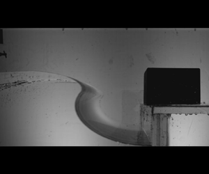
 $x_f \geqslant 0.15 \ \textrm {m}$), were each observed at least twice. Figure 3 presents five frames from a typical test within each impact type.

Figure 3. Images captured from the high-speed movie recording increasing monotonically in time ( $\Delta t = 30 \ \textrm {ms}$) from left to right, for three tests representing the most distinct impact types: broken/aerated (test 2), breaking (test 9a) and sloshing (test 24). (a) Test 2, $x_f = -0.60\ \textrm {m}$, $\Delta x = 12\ \textrm {mm}$. (b) Test 9a, $x_f = -0.05\ \textrm {m}$, $\Delta x = 38\ \textrm {mm}$. (c) Test 24, $x_f = 0.22\ \textrm {m}$, $\Delta x = 11\ \textrm {mm}$.
3.1. Broken (aerated),  $x_f \leqslant -0.6 \ \textrm {m}$

Tests in the broken focus range show the boulder being impacted by a wave whose crest has overturned and impacted the preceding trough prior to the platform (see test 2 of figure 3). Impacts within the broken range are characterised by the slow rise- and decay-time and low amplitude of the pressure time series, as seen in figure 4 for test 2. Figure 5(d) shows the maximum pressure to be low but following an upward trend as  $x_f$ increases into the breaking $x_f$ region. The integrated pressure parameters presented in figure 5(e,f) are variable within the broken region. Without distinct zero up- and down-crossings in the pressure time series, the impact time range is ambiguous and likely the cause of the high variability in the integrated pressure parameters. The $x$-acceleration time series of the boulder is shown for test 2 in figure 4 and is consistently low enough to be indistinguishable from the zero-line. The maximum and integrated parameters of the $x$-acceleration presented in figure 5(a–c) also show low values. However, these are non-zero and boulder displacements of $12.6\ \textrm {mm}$ ( $0.4\ \textrm {m}$ at full scale) and $5.9\ \textrm {mm}$ ( $0.2\ \textrm {m}$ at full scale) were recorded.

Figure 4. Selected pressure (grey line accented with black dots with units of kPa) and  $x$-acceleration (black line with units of $\textrm {m}\ \textrm {s}^{-2}$) time series represented generically in the $y$-axis label by $f(t)$. Time series have been scaled by $C = 2500$ and then translated vertically by the wave focus position, $x_f$. A scale key is given to the left of the $y$-axis. Each test is centred horizontally about its expected time $t_0$ (see § 2.2 for calculation). Coloured areas denote the pressure impact time range of the tests defined in § 2.2. Error bars stretch across twice the impact duration (see § 2.2 for calculation method).

Figure 5. All data points are coloured by boulder displacement (see figure 2). Open circles delineate tests presented in figure 4. The grey circle (clearly visible in some plots) indicates an unknown boulder displacement. (a–c) The  $x$-acceleration maxima and moments. (d–f) Pressure maxima and moments.
3.2. Breaking, $-0.6\ \textrm {m} < x_f < 0.15\ \textrm {m}$

In the breaking  $x_f$ range, the boulder is impacted by breaking waves that consistently exhibit a distinct overturning crest preceded by a smooth trough. A movie of test 14 ( $x_f = 0.05\ \textrm {m}$) can be found in the supplementary material available at https://doi.org/10.1017/jfm.2021.841. Within this range, the tests carried out at $x_f = 0\ \textrm {m}$ were repeated seven times. Additionally, within this $x_f$ range, flip-through events on the boulder were observed.
The pressure time history of test 4 in figure 4 shows a short impact duration of  $2.9\ \textrm {ms}$ and a low single maximum of $29.0\ \textrm {kPa}$ ( $870\ \textrm {kPa}$ at full scale assuming Froude scaling). As $x_f$ is increased, the impact duration increases to a maximum at around test 6 ( $x_f = -0.2 \ \textrm {m}$). From the pressure time histories, the increase in impact duration occurs due to a second pressure peak: it is first seen clearly in test 6. Significant negative pressure values (i.e. below atmospheric pressure) occur following the second pressure peak in the range $-0.2 \ \textrm {m} \leqslant x_f \leqslant 0.1\ \textrm {m}$. From test 7 to test 14 the impact duration decreases significantly from $4.4\ \textrm {ms}$ to $0.4\ \textrm {ms}$. During this contraction of impact duration, the second pressure maximum becomes dominant and the two maxima move closer in time. The concentration of pressure impulse in time is indicative of crest–trough focusing to the same point, i.e. a flip-through impact. Across all tests, the highest pressure maximum of $183\ \textrm {kPa}$ ( $5.5\ \textrm {MPa}$ at full scale) is recorded in test 16 ( $x_f = 0.07\ \textrm {m}$) when the impact duration is also one of the shortest $\sigma _P = 0.29\ \textrm {ms}$ (the shortest being $\sigma _P = 0.26\ \textrm {ms}$ in test 19b, $x_f = 0.09\ \textrm {m}$). Throughout the breaking $x_f$ range, pressure oscillations following the second pressure maximum can be seen in figure 4. These oscillations become more pronounced from test 6 to test 20 and increase in frequency from $200\ \textrm {Hz}$ to $600\ \textrm {Hz}$ giving bubble radii of between $5.6\ \textrm {mm}$ and $15.5 \ \textrm {mm}$ as calculated from (4.5) in Wang et al. (Reference Wang, Ikeda-Gilbert, Duncan, Lathrop, Cooker and Fullerton2018). The three-dimensionality of these experiments allows air to escape along the sides of the boulder following bubble formation, possibly leading to faster oscillation decay than in vertical wall impact experiments (Bogaert et al. Reference Bogaert, Léonard, Brosset and Kaminsk2010; Hattori et al. Reference Hattori, Arami and Yui1994). Cessation of the pressure oscillations at the upper $x_f$ boundary is accompanied by a rapid decrease in the amount of boulder displacement.
The acceleration of the boulder reaches a maximum of  $165\ \textrm {m}\ \textrm {s}^{-2}$ during test 13 where $x_f = 0.04\ \textrm {m}$, and a flip-through impact occurs. However, the boulder displacement in test 13 of $\Delta x = 17.9\ \textrm {mm}$ ( $0.5 \ \textrm {m}$ at full scale) is relatively low. The largest boulder displacements of $38$ and 42 mm in tests 9a and 8a (black data points), respectively, are measured when the pressure impulse is highest ( $0.17 \ \textrm {kPa}\ \textrm {s}$ and $0.18 \ \textrm {kPa}\ \textrm {s}$) being a combination of a high maximum pressure and a long impact duration. Although tests 8a and 9a stand out as having the largest displacements and pressure impulse values, figure 5(e) shows large variability in boulder displacement along the downward trend in pressure impulse. At $x_f = 0\ \textrm {m}$, seven nominally identical tests were carried out where the boulder was displaced by a mean of $22\ \textrm {mm}$ with a standard deviation of $3.5\ \textrm {mm}$. Results are shown in the supplementary material.
3.3. Unbroken (sloshing), $x_f \geqslant 0.15\ \textrm {m}$

Tests in the unbroken  $x_f$ range feature overturning crests that are much less distinct, the wave being unbroken or only marginally breaking at the platform. The images of test 24 in figure 3 show a sloshing impact with little, if any, air entrainment at the boulder face.
The sloshing  $x_f$ range is characterised by long time scale, low-amplitude pressure time series, similar to the aerated regime. While very large pressure peaks in tests 22 and 23 at the boundary of the sloshing region (see test 22 in figure 4) exist, they are not followed by a distinct zero down-crossing, distinguishing the impact from the previous (breaking) $x_f$ region.
Figure 2 shows that the four tests within this  $x_f$ region (tests 22, 23, 24 and 25) follow a largely downward trend to the smallest measured boulder displacement of $4.8\ \textrm {mm}$ ( $0.1\ \textrm {m}$ at full scale). While peak pressure values are high in tests 22 and 23, their short duration does not accelerate the boulder significantly. The lack of pressure oscillations in these tests artificially extends the impact time range, creating variability in the integrated values of figure 5(e,f).
3.4. Error and uncertainty
3.4.1. Anomalous boulder displacement
In figure 2, the two black markers, test 8a and test 9a, have the highest measured boulder displacements of  $42.2\ \textrm {mm}$ ( $1.3\ \textrm {m}$ at full scale) and $38.0 \ \textrm {mm}$ ( $1.1\ \textrm {m}$ at full scale), respectively. In comparison, their repeated counterparts, test 8b and test 9b, have measured boulder displacements $20.5$ and $18.2\ \textrm {mm}$ lower. The standard deviation of boulder displacement across the seven repeated tests at $x_f = 0\ \textrm {m}$ was $3.5\ \textrm {mm}$.
The pressure and acceleration time series parameters presented in figure 5 give no obvious indication as to the cause of the boulder displacement deviance of test 8a and test 9a. In addition to the  $x$-axis acceleration and pressure times series, the $y$- and $z$-axis acceleration time series were inspected, neither showing significant or unusual accelerations. Additionally, the initial positions of the boulder were rechecked using the first frames from each test's high-speed movie. In test 8a, the boulder was found to sit an estimated $2.3 \ \textrm {mm}$ fore of the boulder in test 8b. The standard deviation across initial boulder positions was $0.5\ \textrm {mm}$, implying that boulder position may have been a contributing factor to the anomalous results. From tests 8a and 9a, the boulder displacement's sensitivity to its initial condition could be very high but a stand-alone study is required to conclude this.
3.4.2. Pressure measurement limitations
Previous experiments on flip-through-type impacts have shown how maximum pressure values can be concentrated in very small areas (Lugni et al. Reference Lugni, Brocchini and Faltinsen2006; Wang et al. Reference Wang, Ikeda-Gilbert, Duncan, Lathrop, Cooker and Fullerton2018; Chan & Melville Reference Chan and Melville1988; Cooker Reference Cooker2002). Throughout this experimental campaign, pressure on the boulder was measured at the boulder's front face via a single transducer with a  $5.54 \ \textrm {mm}$ active area diameter. In § 3.2, the minimum bubble radius (associated with the flip-through climax) was estimated at $5.6 \ \textrm {mm}$. High-speed recordings of tests appear to show bubble formation at the transducer location (see the supplementary material for a recording of test 14). However, it is possible for flip-through to focus away from the transducer location, resulting in the measurement of lower maximum pressures. Additionally, in sloshing or fully aerated impacts, pressure rise may appear delayed due to the time taken for fluid to rise up the boulder front face. Such a phenomenon may be the cause of the $x$-axis acceleration increasing approximately $2\ \textrm {ms}$ before the pressure in test 4 (seen in the time series of figure 4).
4. Conclusion
The presented data, obtained by altering the breaking position of a wave impacting a vertical cliff, have demonstrated the influence of wave-impact mode (aerated, breaking or sloshing) on the displacement of clifftop boulders. The largest boulder displacement of  $42\ \textrm {mm}$ ( $1.3\ \textrm {m}$ at full scale) was measured in the breaking $x_f$ range and was associated with two strong pressure peaks spaced at $\approx 4\ \textrm {ms}$ and strong pressure oscillations following the second peak. The smallest boulder displacements were recorded in the broken and unbroken $x_f$ ranges. Across seven nominally identical tests at $x_f = 0$ (in which the pressure parameters were very similar) the boulder was displaced by a mean of $22\ \textrm {mm}$ with a standard deviation of $3.5\ \textrm {mm}$.
This experimental campaign has shown the range of wave focusing positions most conducive to boulder movement and the range of displacement values we may expect in laboratory experiments. The absence of multiple repeated tests and the inability to fully quantify scaling effects mean that future work will firstly seek to reliably extrapolate these laboratory boulder displacement measurements to the real-world scale by quantifying pressure scaling errors using large scale tests, carrying out a larger number of repeated tests, and obtaining frictional similarity between prototype and laboratory scales. Additionally, a comparison between the importance of the wave-breaking position with the significant wave height and peak wave period should be carried out.
Supplementary material
Supplementary material is available at https://doi.org/10.1017/jfm.2021.841.
Acknowledgements
The authors thank A. Disant and E. Bertrand for helping with the laboratory set-up and P. Pergler for help with carrying out the experiments.
Funding
This work was funded by the European Research Council through the HIGHWAVE project (grant no. 833125).
Declaration of interests
The authors report no conflict of interest.


 Open access