


1. Introduction
The migration of a droplet placed on a non-uniformly heated solid surface can be driven by the temperature-induced surface tension gradient. This phenomenon is called thermocapillary migration, which appears in a variety of microfluidic applications (Karbalaei, Kumar & Cho Reference Karbalaei, Kumar and Cho2016). For example, thermocapillary migration has been used in a microfluidic device for droplet and liquid stream actuation on a chemically patterned substrate by Darhuber et al. (Reference Darhuber, Davis, Troian and Reisner2003). They have also proposed a device for droplet production with controlled size (Darhuber, Valentino & Troian Reference Darhuber, Valentino and Troian2010). In addition, several thermocapillary-based microfluidic platforms have been proposed for droplet displacing, switching and trapping (Selva et al. Reference Selva, Miralles, Cantat and Jullien2010), sensing droplet position, size and composition (Chen et al. Reference Chen, Darhuber, Troian and Wagner2004), detection and analysis (Valentino, Troian & Wagner Reference Valentino, Troian and Wagner2005), etc.
Thus, abundant works including theoretical, numerical and experimental studies (Shankar Subramanian & Balasubramaniam Reference Shankar Subramanian and Balasubramaniam2005; Pratap, Moumen & Subramanian Reference Pratap, Moumen and Subramanian2008; Liu & Zhang Reference Liu and Zhang2015; Wu Reference Wu2018) have been carried out on thermocapillary migration due to its practical importance. Dai et al. (Reference Dai, Huang, Wang and Khonsari2021) have reviewed recent advances in the fundamentals, evaluations and manipulation strategies in this field.
Several authors have presented theoretical models of thermocapillary migration. Brochard (Reference Brochard1989) has investigated the motions of droplets on solid surfaces induced by chemical or thermal gradients, and obtained an analytical expression for the migration velocity. Smith (Reference Smith1995) has studied the thermocapillary migration of a two-dimensional liquid droplet on a non-uniformly heated horizontal plate, where the droplet is thin enough so that lubrication theory can be applied to develop an evolution equation for the shape of the free surface. Ford & Nadim (Reference Ford and Nadim1994) have established a model for the thermocapillary migration of a thin two-dimensional droplet having an arbitrary height profile on a solid surface. The thermocapillary motion of spherical-cap drops on horizontal glass surfaces coated with poly(dimethylsiloxane) (PDMS) has been reported by Pratap et al. (Reference Pratap, Moumen and Subramanian2008), and a theoretical description has also been presented. Dai et al. (Reference Dai, Khonsari, Shen, Huang and Wang2016) have carried out experimental and theoretical studies to investigate the migration behaviour of a lubricant droplet induced by a unidirectional thermal gradient. Later, this work was extended to migration induced by an omnidirectional thermal gradient (Dai et al. Reference Dai, Huang, Wang and Khonsari2018) and on radially microgrooved surfaces (Dai et al. Reference Dai, Ji, Huang and Wang2019).
In thermocapillary migration, convection is induced within the droplet. Once the temperature gradient on the free surface exceeds a threshold, the convection will become unstable. Owing to its crucial importance in many applications, especially in crystal growth (Duffar Reference Duffar2010), the thermocapillary instability has received much attention in the past four decades. The related works have been reviewed by Davis (Reference Davis1987), Schatz & Neitzel (Reference Schatz and Neitzel2001) and Lappa (Reference Lappa2009).
Smith & Davis (Reference Smith and Davis1983a) have examined the linear stability of a thermocapillary liquid layer, where an infinite liquid layer on a rigid adiabatic plane is set in motion by imposing a constant temperature gradient on the gas–liquid interface. They found two kinds of instabilities: convective instability (CI) and surface wave instability (SWI). When the free surface is assumed to be non-deformable, CI is dominant, which is driven by mechanisms within the bulk of the layer. In experiments (Riley & Neitzel Reference Riley and Neitzel1998) and numerical simulations (Li et al. Reference Li, Imaishi, Azami and Hibiya2004), hydrothermal waves of CI have been observed. The mechanism of CI is purely hydrodynamic at small Prandtl numbers (Pr), but hydrothermal at large Pr (Wanschura et al. Reference Wanschura, Shevtsova, Kuhlmann and Rath1995; Yan, Hu & Chen Reference Yan, Hu and Chen2018). Chan & Chen (Reference Chan and Chen2010) have performed a linear stability analysis of thermocapillary–buoyancy convection in a horizontal fluid layer. The critical parameters they obtained agree with the experimental results reported by Riley & Neitzel (Reference Riley and Neitzel1998).
On the other hand, when surface deformation is considered, SWI can occur. Smith & Davis (Reference Smith and Davis1983b) have investigated the two-dimensional mode that couples the interfacial deflection to the base flow. It has been found that SWI is most prominent at low Pr and is hydrodynamic in nature (Davis Reference Davis1987). Later, Patne, Agnon & Oron (Reference Patne, Agnon and Oron2020, Reference Patne, Agnon and Oron2021a) have generalized this work to three-dimensional disturbances for a liquid layer subjected to an oblique temperature gradient and the case of a viscoelastic fluid (Reference Patne, Agnon and Oron2021b).
There are also some experiments on SWI. Duan, Kang & Hu (Reference Duan, Kang and Hu2006) have performed an experimental study on the surface deformation in thermocapillary convection, which proves that SWI exists on the free surface. Zhu et al. (Reference Zhu, Zhou, Duan and Kang2011) have reported the surface oscillation of thermocapillary convection in a rectangular pool of silicone oil. Bach & Schwabe (Reference Bach and Schwabe2015) have reviewed and complemented the experimental results on SWI in thermocapillary annular gaps, which show that surface waves exhibit a considerably larger frequency, phase speed and surface deformation amplitude compared to hydrothermal waves.
The controllability of a droplet is highly dependent on the stability of the flow during migration. Determining the critical parameters of the transition and instability mechanism will enrich our understanding of droplet dynamics, and guide future development of microfluidics. However, to our best knowledge, few works have been carried out in this field. The only one we know is our previous study on the CI of thermocapillary–buoyancy convection in droplet migration (Hu, Yan & Chen Reference Hu, Yan and Chen2019), where hydrothermal waves are detected at critical Marangoni numbers.
In the present work, we would like to pay attention to the SWI of thermocapillary migration. Although SWI in thermocapillary convection is an existing problem, previous works have been confined to a few cases of liquid layers, and experiments reporting SWI are limited. Therefore, the understanding of SWI is very in adequate. The surface deflection cannot tell us directly whether the instability belongs to SWI, as some experiments show that faint surface oscillations can be found in CI and sometimes SWI can coexist with CI (Bach & Schwabe Reference Bach and Schwabe2015). The properties of and the instability mechanism for SWI need to be clarified. The present work suggests that the kind of instability depends on several parameters besides the capillary number Ca, which measures the surface deflection. In addition, we find new modes and mechanisms that can enrich the understanding of SWI in thermocapillary convection. In many applications of droplet migration, the fluids are polymeric liquids. Thus, both a Newtonian fluid and a viscoelastic fluid are considered in our investigation.
The paper is arranged as follows. In § 2, the problem statement and dimensionless governing equations are introduced. The base-state solution and perturbation equations are derived. After that, critical parameters, perturbation fields and energy mechanisms are presented in § 3. Later, we discuss the instability mechanism and make comparisons with available experiments in § 4. Finally, major conclusions are summarized in § 5.
2. Problem formulation
Referring to figure 1, we consider a thin droplet on a horizontal plane with a temperature gradient in the x direction (Dai et al. Reference Dai, Khonsari, Shen, Huang and Wang2016); y and z are the spanwise and wall-normal directions, respectively. As a simplification, we assume that the droplet is an infinitely long strip in the y direction with width L and thickness d (Ford & Nadim Reference Ford and Nadim1994). The liquid is in contact with an inviscid atmosphere. Suppose the surface tension varies linearly with the temperature T:
 \begin{equation}\sigma ^{\prime} = {\sigma ^{\prime}_0} - \gamma (T - {T_0}),\end{equation}
where γ is the surface tension coefficient. Thus, the droplet can be set in motion by the thermocapillary effect.

Figure 1. Side view of thermocapillary migration for a thin droplet on a solid plane. The droplet can be susceptible to SWI when its surface is deformable.
In the vicinity of the three-phase contact line,  ${\varphi _a}$ and ${\varphi _r}$ are the advancing and receding contact angles, respectively. Contact angle hysteresis is found in many droplet migrations (Chen et al. Reference Chen, Troian, Darhuber and Wagner2005; Pratap et al. Reference Pratap, Moumen and Subramanian2008). However, Brzoska, Brochard-Wyart & Rondelez (Reference Brzoska, Brochard-Wyart and Rondelez1993) have shown that typical contact angle hysteresis is $\tilde{\delta } = \cos {\varphi _a} - \cos {\varphi _r} = 1.5 \times {10^{ - 2}}$ for silicone oils and $\tilde{\delta } = {10^{ - 2}}$ for n-alkanes, while the variations of contact angle with temperature are extremely small. As the difference between ${\varphi _a}$ and ${\varphi _r}$ is not crucial for the stability analysis, we assume that ${\varphi _a} = {\varphi _r} = \varphi $ for simplicity in the following.
Generally, the droplet has an oval shape. However, when L is much larger than the capillary length  ${\hat{\kappa }^{ - 1}} = \sqrt {{{\sigma ^{\prime}}_0}/({\rho _0}g)} $, the droplet can be flattened by gravity and forms a pancake, while the thickness in the base state is a constant $d = 2{\hat{\kappa }^{ - 1}}\sin (\varphi /2)$ except in the rim of the droplet (Brochard Reference Brochard1989). Here, ${\sigma ^{\prime}_0}$, ${\rho _0}$ and g are the surface tension, fluid density and gravitational acceleration, respectively. This can also be seen in the experiment (figure 2 of Dai et al. Reference Dai, Khonsari, Shen, Huang and Wang2016). Thus, d is assumed to be a constant. In addition, we consider the case when $\varphi $ is not too small, so that d has the same order as ${\hat{\kappa }^{ - 1}}$, and $L \gg d$.
2.1. Governing equations
We suppose that the liquid is an incompressible fluid, whose dynamic viscosity  $\mu $ and thermal diffusivity $\chi $ are constants. Both a Newtonian fluid and a viscoelastic fluid are considered in the following. The latter is modelled by an Oldroyd-B fluid, which can be derived from the kinetic theory for a dilute suspension of polymer molecules in a Newtonian solvent (Bird, Armstrong & Hassager Reference Bird, Armstrong and Hassager1987).
The dimensionless numbers can be given as follows:
 \begin{gather}Ma = \frac{{b\gamma {d^2}}}{{\chi \mu }},\quad Pr = \frac{\mu }{{\rho \chi }},\quad R = \frac{{Ma}}{{Pr}} = \frac{{\rho Ud}}{\mu },\quad S = \frac{{\rho d{{\sigma ^{\prime}}_0}}}{{{\mu ^2}}},\end{gather}
 \begin{gather}Ca = \frac{{Ma}}{{Pr{\mkern 1mu} {\mkern 1mu} S}},\quad G = \frac{{\rho g{d^2}}}{{\mu U}},\quad Bo = \frac{{{\rho _0}g\kappa {d^2}}}{\gamma }.\end{gather}
Here, Ma is the Marangoni number, which measures the thermocapillary effect; b is the temperature gradient on the plane; Pr is the Prandtl number; R is the Reynolds number; S is the non-dimensional surface-tension number;  $U = b\gamma d/\mu $ is the velocity scale; and Ca is the capillary number, which measures the magnitude of the surface deformation (Smith & Davis Reference Smith and Davis1983a). When S is large enough, $Ca \to 0$ and the surface deformation can be neglected, and CI rather than SWI is preferred. However, when $O(Ca) \ge 0.001$, the surface wave can be the preferred mode in some cases (Smith & Davis Reference Smith and Davis1983b). Also above, G is the Galileo number, which measures the gravity effect; and Bo is the dynamic Bond number, which measures the buoyancy effect. Suppose the fluid density varies linearly with the temperature,
 \begin{equation}\rho = {\rho _0}[1 - \kappa (T - {T_0})],\end{equation}
where κ is the thermal expansion coefficient. We can see that Bo is independent of the surface tension gradient. Although the fluid is assumed to be incompressible, the variation of density with temperature in the presence of gravity can lead to a buoyancy effect, which may change the flow significantly. So the Boussinesq approximation is used.
The dimensionless governing equations can be obtained as follows, which are the continuity equation, the momentum equation and the energy equation, respectively (Yan et al. Reference Yan, Hu and Chen2018); the scales of non-dimensionalization are presented in table 1:
 \begin{gather}\boldsymbol{\nabla }\boldsymbol{\cdot }\boldsymbol{u} = 0,\end{gather}
 \begin{gather}R\left( {\frac{{\partial \boldsymbol{u}}}{{\partial t}} + \boldsymbol{u}\boldsymbol{\cdot }\boldsymbol{\nabla }\boldsymbol{u}} \right) ={-} \boldsymbol{\nabla }p + \boldsymbol{\nabla }\boldsymbol{\cdot }\boldsymbol{\tau } + (Bo{\mkern 1mu} {\mkern 1mu} T - G)\boldsymbol{\nabla }z,\end{gather}
 \begin{gather}\frac{{\partial {\kern 1pt} T}}{{\partial {\kern 1pt} t}} + \boldsymbol{u}\boldsymbol{\cdot }\boldsymbol{\nabla }T = \frac{1}{{Ma}}{\nabla ^2}T.\end{gather}
Table 1. The scales of non-dimensionalization.

Here, u = (u, v, w), p, T and  $\boldsymbol{\tau }$ stand for the velocity, pressure, temperature and stress, respectively. The buoyancy effect is taken into account in the momentum equation (Hu et al. Reference Hu, He, Chen and Liu2018). When $G \gg L/d$, we have $\rho gd \gg (\mu U/{d^2})L$, which means that the variation of pressure along the x direction is much smaller than the pressure caused by gravity. Thus, the thickness expression $d = 2{\hat{\kappa }^{ - 1}}\textrm{sin}(\varphi /2)$ derived by Brochard (Reference Brochard1989) is still valid for droplet migration.
For example, the values of physical and dimensionless parameters for liquid silicon (Smith & Davis Reference Smith and Davis1983b) are stated in table 2. Here, we set the values of  $\varphi $, b and L. It can be seen that the dimensionless parameters Pr, R, S, Ca, Ma and G are within the ranges we will consider in this paper. In addition, $L \gg {\hat{\kappa }^{ - 1}},d$ and $G \gg L/d$, while the variation of surface tension along the x direction is small: $bL\gamma \ll {\sigma ^{\prime}_0}$.
Table 2. The values of physical and dimensionless parameters for liquid silicon.

The dimensionless constitutive equation for a Newtonian fluid is
 \begin{equation}\boldsymbol{\tau } = \boldsymbol{S},\end{equation}
where  ${\textstyle{1 \over 2}}\boldsymbol{S} = {\textstyle{1 \over 2}}[\boldsymbol{\nabla }\boldsymbol{u} + {(\boldsymbol{\nabla }\boldsymbol{u})^\textrm{T}}]$ is the strain-rate tensor. For an Oldroyd-B fluid, one has
 \begin{equation}\left( {1 + \lambda \frac{{\delta {\kern 1pt} }}{{\delta {\kern 1pt} t}}} \right)\boldsymbol{\tau } = \left( {1 + \lambda \tilde{\beta }\frac{{\delta {\kern 1pt} }}{{\delta {\kern 1pt} t}}} \right)\boldsymbol{S},\end{equation}
where  $\delta {\kern 1pt} /\delta t$ is the upper convected derivative with the expression
 \begin{equation}\frac{{\delta \boldsymbol{\tau }}}{{\delta t}} = \frac{{\partial \boldsymbol{\tau }}}{{\partial t}} + \boldsymbol{u}\boldsymbol{\cdot }\boldsymbol{\nabla }\boldsymbol{\tau } - {(\boldsymbol{\nabla }\boldsymbol{u})^\textrm{T}}\boldsymbol{\cdot }\boldsymbol{\tau } - \boldsymbol{\tau }\boldsymbol{\cdot }(\boldsymbol{\nabla }\boldsymbol{u}).\end{equation}
Here,  $\lambda = (\mu /\tilde{G})(U/d)$ is the Weissenberg number, $\tilde{G}$ is the elastic modulus and $\tilde{\beta }$ is the ratio of solvent viscosity to total viscosity. The elasticity number $\varepsilon = \lambda /R$ is used in the following, as it depends only on the properties of the fluid and the geometry. When $\lambda = 0$ or $\tilde{\beta } = 1$, the Oldroyd-B fluid recovers the Newtonian fluid.
We choose the reference frame travelling with the droplet, while the plane moves at the speed of  $\zeta $ in the negative x direction. Thus, the flux in the x direction is zero: $\int_0^1 {u\,\textrm{d}z} = 0$. The boundary conditions on the rigid plane are
 \begin{equation}u{|_{z = 0}} ={-} \zeta ,\quad T{|_{z = 0}} ={-} x,\end{equation}
where  $\zeta $ is the dimensionless migration velocity and a temperature gradient is imposed on the plane. We suppose that a deformable gas–liquid interface is located at $z = 1 + \xi (x,y,t)$, where $\xi (x,y,t)$ is the small displacement of the interface from its undisturbed position $z = 1$. The boundary conditions at the interface are presented as follows, which are the kinematic boundary condition, the tangential and normal components of the stress balance (Pérez-García & Carneiro Reference Pérez-García and Carneiro1991) and the continuity of heat flux, respectively:
 \begin{gather}{\partial _t}\xi + {\boldsymbol{u}_ \bot }\boldsymbol{\cdot }\boldsymbol{\nabla }\xi = w,\end{gather}
 \begin{gather}{\boldsymbol{t}_j}\boldsymbol{\cdot }\boldsymbol{\tau }\boldsymbol{\cdot }\boldsymbol{n} ={-} \boldsymbol{\nabla }T\boldsymbol{\cdot }{\boldsymbol{t}_j},\end{gather}
 \begin{gather}- p + \boldsymbol{n}\boldsymbol{\cdot }\boldsymbol{\tau }\boldsymbol{\cdot }\boldsymbol{n} ={-} C{a^{ - 1}}({\boldsymbol{\nabla }_s}\boldsymbol{\cdot }\boldsymbol{n}) - G\xi ,\end{gather}
 \begin{gather}- \boldsymbol{\nabla }T\boldsymbol{\cdot }\boldsymbol{n} = 0.\end{gather}
In (2.11a),  ${\boldsymbol{u}_ \bot } = (u,v)$ is the two-dimensional velocity in the x–y plane; (2.11b) stands for the shear stress caused by the thermocapillary effect; and ${\boldsymbol{t}_j}$ and $\boldsymbol{n}$ are the unit tangent and unit normal vectors to the free surface, respectively. Their linearized expressions in the perturbed state are (Patne et al. Reference Patne, Agnon and Oron2021a)
 \begin{equation}\boldsymbol{n} ={-} {\partial _x}\xi {\boldsymbol{e}_x} + {\boldsymbol{e}_z} - {\partial _y}\xi {\boldsymbol{e}_y},\quad {\boldsymbol{t}_{1}} = {\boldsymbol{e}_x} + {\partial _x}\xi {\boldsymbol{e}_z},\quad {\boldsymbol{t}_{2}} = {\partial _y}\xi {\boldsymbol{e}_z} + {\boldsymbol{e}_y}.\end{equation}
In (2.11c),  ${\boldsymbol{\nabla }_s} = (\boldsymbol{I} - \boldsymbol{nn})\boldsymbol{\cdot }\boldsymbol{\nabla }$ is the surface gradient operator; and finally (2.11d) stands for zero heat flux.
We restrict our attention to flow that is not near the rim of the droplet. Thus, the basic flow is assumed to be parallel, while the temperature is linear in x plus a distribution in z as follows:
 \begin{equation}\boldsymbol{u} = ({U_0}(z),0,0),\quad {T_0}(x,z) ={-} x + {T_b}(z).\end{equation}
The velocity and temperature distributions for the base state can be determined as follows (Hu et al. Reference Hu, Yan and Chen2019):
 \begin{gather}{U_0}(z) ={-} \zeta \left( {1 - 3z + \frac{3}{2}{z^2}} \right) + \left( { - \frac{1}{2}z + \frac{3}{4}{z^2}} \right) + \frac{{Bo}}{4}\left( { - \frac{1}{2}z + \frac{5}{4}{z^2} - \frac{2}{3}{z^3}} \right),\end{gather}
 \begin{gather}{T_b}(z) = {z^2}Ma\left[ {\frac{\zeta }{8}{{( - 2 + z)}^2} + \frac{z}{4}\left( {\frac{1}{3} - \frac{1}{4}z} \right) + \frac{{Bo}}{{24}}\left( {\frac{1}{2}z - \frac{5}{8}{z^2} + \frac{1}{5}{z^3}} \right)} \right].\end{gather}
It is found that the average of the velocity gradient and the surface temperature increase with Bo and  $\zeta $, while the upper surface is hotter than the bottom.
When Bo = 0, the velocity distribution (2.14a) agrees with equation (8) of Pratap et al. (Reference Pratap, Moumen and Subramanian2008). The above solutions are the same for the Newtonian fluid and the Oldroyd-B fluid. However, due to the elasticity, there is a normal stress component for the latter. The total stress tensor accounting for both Newtonian and elastic contributions can be given as follows:
 \begin{equation}{\boldsymbol{\tau }_0} = \left[ {\begin{array}{*{20}{c}} {{{\bar{\tau }}_{11}}}&0&{{{\bar{\tau }}_{13}}}\\ 0&0&0\\ {{{\bar{\tau }}_{13}}}&0&0 \end{array}} \right],\end{equation}
where  ${\bar{\tau }_{13}} = \textrm{D}{U_0}(z)$ and ${\bar{\tau }_{11}} = 2\lambda (1 - \tilde{\beta }){[\textrm{D}{U_0}(z)]^2}$ with $\textrm{D}{U_0}(z) = (\textrm{d}/\textrm{d}z){U_0}(z)$.
The migration velocity can be derived as follows:
 \begin{equation}\zeta = \frac{{2\textrm{cos}\phi + 1}}{6} + \frac{1}{{24}}Bo,\end{equation}
where the details can be found in Hu et al. (Reference Hu, Yan and Chen2019) and Dai et al. (Reference Dai, Khonsari, Shen, Huang and Wang2016).
2.2. Perturbed state
Now we apply an infinitesimal three-dimensional disturbance in the normal mode form to the base state:
 \begin{gather}(\boldsymbol{u},T,P,\boldsymbol{\tau },z) = ({\boldsymbol{u}_0},{T_0},{P_0},{\boldsymbol{\tau }_0},\textrm{1}) + \boldsymbol{\delta },\end{gather}
 \begin{gather}\boldsymbol{\delta } = (\mathord{\buildrel{\lower3pt\hbox{$\scriptscriptstyle\frown$}} \over u} ,\mathord{\buildrel{\lower3pt\hbox{$\scriptscriptstyle\frown$}} \over v} ,\mathord{\buildrel{\lower3pt\hbox{$\scriptscriptstyle\frown$}} \over w} ,\mathord{\buildrel{\lower3pt\hbox{$\scriptscriptstyle\frown$}} \over T} ,\mathord{\buildrel{\lower3pt\hbox{$\scriptscriptstyle\frown$}} \over P} ,\boldsymbol{\mathord{\buildrel{\lower3pt\hbox{$\scriptscriptstyle\frown$}} \over \tau } },\mathord{\buildrel{\lower3pt\hbox{$\scriptscriptstyle\frown$}} \over \xi } )\textrm{exp[}\sigma t + \textrm{i(}\alpha x + \beta y\textrm{)]},\end{gather}
where the subscript 0 stands for the basic flow while the variables without subscript 0 refer to the perturbation. The complex eigenvalue  $\sigma = {\sigma _r} + \textrm{i}{\sigma _i}$ consists of the growth rate ${\sigma _r}$ and the frequency ${\sigma _i}$. The parameters $\alpha $ and $\beta $ are the wavenumbers in the x and y directions, respectively. The total wavenumber, wave speed and wave propagation angle are defined as $k = \sqrt {{\alpha ^2} + {\beta ^2}} $, $c = |{{\sigma_i}} |/k$ and $\theta = \textrm{ta}{\textrm{n}^{ - 1}}(\beta /\alpha )$, respectively. Owing to the symmetry, we only need to consider the case $\theta \in \textrm{[}0\mathrm{^\circ },180\mathrm{^\circ }\textrm{)}$. The perturbation equations have been presented in Hu et al. (Reference Hu, He, Chen and Liu2018) and the boundary conditions are described in the Appendix.
The Chebyshev collocation method (Schmid & Henningson Reference Schmid and Henningson2001) is used to solve the general eigenvalue problem in the form of  $\boldsymbol{\mathsf{W}}\boldsymbol{g} = \sigma \boldsymbol{\mathsf{Z}}\boldsymbol{g}$, where W and Z are two matrices, and $\boldsymbol{g}$ is the eigenvector. We set Nc Gauss–Lobatto points for the governing equations in the flow region $z = [1 - \cos (j{\rm \pi} /({N_c} + 1))]/2$, $j = 1- {N_c}$, and two points for the boundary conditions at z = 0,1 (2.25). The results are sufficiently accurate when ${N_c} = 80-100$.
In order to validate our code, we compute some parameters of the two-dimensional SWI in the thermocapillary liquid layer in table 3 and the critical parameters of CI in the thermocapillary–buoyancy convection in table 4. The code for the constitutive equations of an Oldroyd-B fluid is validated by computing the critical parameters of plane Poiseuille flow for the Oldroyd-B fluid in table 5. Most of perturbation equations in the liquid layer and the channel flow are the same as those in the droplet migration, so we only need to change the basic flow and some boundary conditions in the code. Comparisons are made with the results of Smith & Davis (Reference Smith and Davis1983b), Riley & Neitzel (Reference Riley and Neitzel1998), Chan & Chen (Reference Chan and Chen2010) and Sureshkumar & Beris (Reference Sureshkumar and Beris1995). Our results are comparable to those in the previous works.
Table 3. Some parameters of the two-dimensional SWI in thermocapillary liquid layers: (a) critical parameters of the linear flow; and (b) neutral Reynolds numbers of the return flow. Here, ‘SD’ and ‘PW’ stand for the results of Smith & Davis (Reference Smith and Davis1983b) and the present work, respectively.

Table 4. The critical parameters of CI in the thermocapillary–buoyancy convection at  $Pr = 13.9$ and $Bo = 0.142$. Here, ‘RN’, ‘CC’ and ‘PW’ stand for the results of Riley & Neitzel (Reference Riley and Neitzel1998), Chan & Chen (Reference Chan and Chen2010) and the present work, respectively.

Table 5. The critical parameters of plane Poiseuille flow for the Oldroyd-B fluid ( $\tilde{\beta } = 0.5$, $\beta = 0$). Our results are exactly the same as those in Sureshkumar & Beris (Reference Sureshkumar and Beris1995).

3. Numerical results
We determine the neutral Marangoni numbers MaN of neutral modes  $({\sigma _r} = 0)$. Then, the critical Marangoni number Mac can be obtained, which is the global minimum of MaN for all $\textrm{(}\alpha ,\beta \textrm{)}$:
 \begin{equation}M{a_c} = \mathop {\textrm{min}}\limits_{\alpha ,\beta } M{a_N}(\zeta ,Pr,G,Ca,Bo,\varepsilon ).\end{equation}
The flow is linearly stable for any modes when Ma < Mac.
The computation suggests that there are two kinds of instability: CI and SWI. The former has been examined in our previous work (Hu et al. Reference Hu, Yan and Chen2019). For the latter, two kinds of preferred modes are detected, which are the streamwise wave ( $\theta = 0\mathrm{^\circ }$ or $180\mathrm{^\circ }$) and the oblique wave ( $\theta \ne 0\mathrm{^\circ }$, $90\mathrm{^\circ }$ and $180\mathrm{^\circ }$). The results for the Newtonian fluid and for the Oldroyd-B fluid are presented in §§ 3.1 and 3.2, respectively.
3.1. Newtonian fluid
3.1.1. The effect of the Galileo number
First, we study the effect of the Galileo number G on the instability. The variation of Mac with Pr at  $\zeta = 0.49$, Ca = 0.001 and Bo = 0 is displayed in figure 2. It can be seen that Mac always increases with Pr. SWI is preferred at Pr < 19.1 for G = 10 and Pr < 2.05 for G = 100. The preferred mode is the downstream streamwise wave ( $\theta = 0\mathrm{^\circ }$, curves a and b in figure 2), and Mac increases with G. When Pr becomes larger, the preferred mode changes to the oblique wave of CI (curve c in figure 2), which is independent of G. When G = 1000, we can only find CI in the flow.

Figure 2. The variation of Mac with Pr at  $\zeta = 0.49$, Ca = 0.001 and Bo = 0. The curves correspond to streamwise waves of SWI (a and b) and the oblique wave of CI (c).
In figure 3, we show the wavenumber, propagation angle and wave speed of the preferred modes. It can be seen that, for SWI, the wavenumbers are less than 0.6. The wave speeds increase significantly with Pr. For CI, the wavenumbers are of the order of 2, the oblique wave travels upstream  $(90\mathrm{^\circ } < \theta < 180\mathrm{^\circ })$ and the wave speed is much smaller than those of SWI. We will confine ourselves to the case of G = 100 in the following study.

Figure 3. The (a) wavenumber and (b) wave speed of the modes in figure 2.
3.1.2. The effect of the surface-tension number
In this section, we study the effect of the surface-tension number S. The variation of Mac with S is displayed in figure 4. The dashed portions of curves a and e are where the condition (A3) is not satisfied. When Pr = 0.01, the preferred mode includes the streamwise waves (curves a and c in figure 4) and the oblique waves (curves b and d in figure 4). Here, curve b belongs to the SWI whose propagation angle has  $\theta \in (0\mathrm{^\circ },40\mathrm{^\circ })$. When S is large enough, the preferred mode changes from SWI to CI. When Pr = 1, the SWI is more prominent at S < 3.39 × 10⁵ (curve e in figure 4). When Pr = 100, only the CI is found. There are two kinds of streamwise waves, which travel upstream ( $\theta = 180\mathrm{^\circ }$, curve a) and downstream ( $\theta = 0\mathrm{^\circ }$, curves c and e), respectively.

Figure 4. The variation of Mac with S at  $\zeta = 0.49$ and Bo = 0. The curves correspond to streamwise waves (a, c and e) and oblique waves (b, d,f and g). SWI includes curves a, b, c and e, while CI includes curves d,f and g. The dashed portions of curves a, e and g are where the condition (A3) is not satisfied.
The wavenumber and wave speed of the preferred modes are displayed in figure 5. In the following, we will confine ourselves to the case Ca = R/S = 0.001, so that the condition (A3) can always be satisfied.

Figure 5. The (a) wavenumber and (b) wave speed of the modes in figure 4.
3.1.3. The effects of the migration velocity and the Bond number
The effects of the migration velocity  $\zeta $ and the Bond number Bo are discussed in this section.
(A)  $Pr=0.01$
The variations of Mac with  $\zeta $ and Bo at Pr = 0.01 are displayed in figure 6. It can be seen from (2.16) that the region of $\zeta $ depends on Bo. The Mac value always decreases with Bo. When Bo = 0, the variation of Mac with $\zeta $ is non-monotonic. The preferred modes include the streamwise waves of SWI (curves a and c in figure 6) and the oblique wave of CI (curve b in figure 6). Here, curves a and b correspond to the wave travelling upstream $(\theta > 90\mathrm{^\circ })$ while curve c corresponds to the wave travelling downstream $(\theta < 90\mathrm{^\circ })$. When Bo = 5 and 10, Mac always decreases with $\zeta $. The preferred modes are the downstream streamwise waves of SWI (curves d and e in figure 6).

Figure 6. The variation of Mac with  $\zeta $ and Bo at Pr = 0.01. The curves correspond to streamwise waves of SWI (a, c, d and e) and the oblique wave of CI (b).
The wavenumber and wave speed of the preferred modes in figure 6 are displayed in figure 7. It can be seen that the wavenumbers of SWI (curves a, c, d and e in figure 7) are much smaller than those of CI (curve b in figure 7), while the reverse is true for the wave speed.

Figure 7. The (a) wavenumber and (b) wave speed of the modes in figure 6.
The wavenumbers of curves a, d and e in figure 7 tend to zero, which means that they belong to the long-wave instability. For these modes, MaN increases with k. However, the wavenumber of SWI cannot be arbitrarily small. Owing to (A3),  $k \gg Ca \times \mathrm{2}{\rm \pi} \approx 0.006$. In addition, the largest wavelength is the width L, which leads to $k \ge \mathrm{2}{\rm \pi} d/L$. Therefore, the actual Mac will be larger than the value shown in figure 6. When Bo = 0 and $\zeta = 0$, the Mac of CI is 19.38. Thus, SWI is preferred when $k < 0.094$. If this value does not satisfy the previous requirements, CI will be preferred.
Here, the perturbation flow fields of the preferred modes at Pr = 0.01 are plotted in figure 8. It can be seen that there are hot spots on the surface. In figure 8(a) (respectively, figure 8b,c), the vertical up-flow on the surface at the phase  $\phi = 3.5$ make $\xi $ increase, so the wave travels upstream (respectively, downstream), while the hot spot is near the wave trough (respectively, crest). There is no roll in the flow field, which is different from the case of CI. The modes in figures 8(a) and 8(b) belong to the long-wave instability.

Figure 8. The perturbation flow field and surface deformation at Pr = 0.01, Ca = 0.001 and G = 100: (a) Bo = 0,  $\zeta = 0$; (b) Bo = 10, $\zeta = 0.5$; and (c) Bo = 0, $\zeta = 0.49$. The perturbation phase is defined as $\phi = \alpha x + \beta y$.
(B)  $Pr=1$
Figure 9 shows Mac at Pr = 1. The variation of Mac with Bo is non-monotonic; and Mac decreases with  $\zeta $ except for the case at Bo = 0, $\zeta < - 0.025$. The preferred modes include the streamwise waves of SWI (curves a, c, e and f in figure 9) and the oblique waves of CI (curves b and d in figure 9). Here, curves a, b and d travel upstream, while curves c, e and f travel downstream.

Figure 9. The variation of Mac with  $\zeta $ and Bo at Pr = 1. The curves correspond to streamwise waves of SWI (a, c, e and f) and oblique waves of CI (b and d).
The wavenumber and wave speed of the preferred modes in figure 9 are displayed in figure 10. Here, curves a, e and f in figure 10 belong to the long-wave instability. Once again, the wavenumbers (wave speeds) of SWI are much smaller (larger) than those of the CI.

Figure 10. The (a) wavenumber and (b) wave speed of the modes in figure 9.
(C)  $Pr=100$
The variations of Mac with  $\zeta $ and Bo at Pr = 100 are displayed in figure 11. The preferred modes include the streamwise waves of SWI (curves a, c and d in figure 11) and the oblique wave of CI (curve b in figure 11). Here, curves a and b travel upstream, while curves c and d travel downstream. SWI is dominant at Bo > 0.

Figure 11. The variation of Mac with  $\zeta $and Bo at Pr = 100. The curves correspond to streamwise waves of SWI (a, c and d) and the oblique wave of CI (b).
The wavenumber and wave speed of the preferred modes in figure 11 are displayed in figure 12. Here, curves a and d in figure 12 belong to the long-wave instability. For SWI, the wave speed increases with  $\zeta $ when Bo > 0. The relationship between SWI and CI is similar to the cases at Pr = 0.01 and 1.

Figure 12. The (a) wavenumber and (b) wave speed of the modes in figure 11.
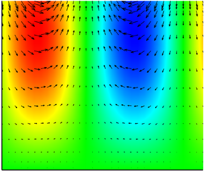
When Bo > 0, there is a new type of perturbation field, which is displayed in figure 13. We can find two hot spots in the vertical direction (z = 0.5 and 0.9). There are two rolls in one cycle  $(\phi \in [0,2{\rm \pi}])$, which almost coincide with the isothermals.

Figure 13. The perturbation flow field and surface deformation at Pr = 100,  $\zeta = 0.4$, Bo = 5, Ca = 0.001 and G = 100. The preferred mode is the downstream streamwise wave. Here, Ts is the perturbation temperature on the surface.
3.1.4. Energy analysis
The energy mechanism of SWI is studied in this section. The rate of change for the perturbation energy can be derived as follows (Wanschura et al. Reference Wanschura, Shevtsova, Kuhlmann and Rath1995; Hu, Peng & Zhu Reference Hu, Peng and Zhu2012):
 \begin{align} \dfrac{{\partial {E_{kin}}}}{{\partial t}} & ={-} \dfrac{1}{R}\int {p\boldsymbol{u}\boldsymbol{\cdot }\boldsymbol{n}\,{\textrm{d}^2}r} - \dfrac{1}{{2R}}\int {\textrm{(}\boldsymbol{\tau }\ {\bf :}\ \boldsymbol{S}\textrm{)}\,{\textrm{d}^3}r} + \dfrac{1}{R}\int {\boldsymbol{u}\boldsymbol{\cdot }\boldsymbol{\tau }\boldsymbol{\cdot }\boldsymbol{n}\,{{\rm d}^2}r} \nonumber\\ & \quad - \int {\boldsymbol{u}\boldsymbol{\cdot }[(\boldsymbol{u}\boldsymbol{\cdot }\boldsymbol{\nabla }){\boldsymbol{u}_0}]\,{\textrm{d}^3}r} + \int {\left( {\dfrac{{Bo}}{R}T{\kern 1pt} {\boldsymbol{e}_3}\boldsymbol{\cdot }\boldsymbol{u}} \right)\,{\textrm{d}^3}r} \nonumber\\ & = P - N + M + I + B. \end{align}
Here, P is the work done by the pressure on the surface, N is the work done by stress in the bulk of the layer, M is the work done by stress on the surface, I is the energy from the basic flow, and B is the work done by the buoyancy (Hu et al. Reference Hu, He, Chen and Liu2018); and  $\int {f\,{\textrm{d}^2}r} $ and $\int {f\,{\textrm{d}^3}r} $ stand for the surface and volume integrals, respectively. For the Newtonian fluid, $\boldsymbol{\tau } = \boldsymbol{S}$, so N > 0, which stands for the viscous dissipation. The perturbation is normalized as $\int {{{|\boldsymbol{u} |}^2}\,{\textrm{d}^3}r} = 1$.
As the stress on the deformed surface has horizontal and vertical components, M can be decomposed into two terms as follows:
 \begin{equation}M = \frac{1}{R}\int {(u{\tau _{13}} + v{\tau _{23}})\,{\textrm{d}^2}r} + \frac{1}{R}\int {w{\tau _{33}}\,{\textrm{d}^2}r} = {M_h} + {M_v}.\end{equation}
In addition, we can see from (A2b) and (A2c) that shear stress can be induced by the Marangoni effect and the surface deformation. Thus, Mh is decomposed into the following two terms:
 \begin{gather}{M_h} = {M_{h,T}} + {M_{h,\xi }},\end{gather}
 \begin{gather}{M_{h,T}} = \frac{1}{R}\int {\left[ {u\left( { - \frac{{\partial T}}{{\partial x}}} \right) + v\left( { - \frac{{\partial T}}{{\partial x}}} \right)} \right]\,{\textrm{d}^2}r} ,\end{gather}
 \begin{gather}{M_{h,\xi }} = \frac{1}{R}\int {\left[ {u( - {\partial_z}{T_0} + {{\bar{\tau }}_{11}})\frac{{\partial \xi }}{{\partial x}} - u\frac{{\partial {{\bar{\tau }}_{13}}}}{{\partial z}}\xi + v( - {\partial_z}{T_0})\frac{{\partial \xi }}{{\partial y}}} \right]\,{\textrm{d}^2}r} .\end{gather}
 Table 6 shows the terms of perturbation energy growth for SWI. It can be seen that M is often the main energy source, I is important in some cases at small Pr, while B is negligible; P always leads to dissipation. The maximum of  $|{P/N} |$ is 12 %, while $|{P/N} |< 3\,\%$ in most cases, so P is not essential for the energy mechanism. Also, Mh is much larger than Mv. For the long-wave mode (cases 1 and 5), Mh is caused by the surface deformation, while for the mode with finite wavelength (cases 2, 3 and 4), it is caused by the Marangoni effect.
Table 6. The terms of the perturbation energy growth for SWI: case 1,  $Pr = 0.01,\, Bo = 0,\, \zeta = 0$; case 2, $Pr = 0.01,\, Bo = 0,\, \zeta = 0.49$; case 3, $Pr = 1,\, Bo = 0,\, \zeta = 0.35$; case 4, $Pr = 100,\, Bo = 5,\, \zeta = 0.4$; and case 5, $Pr = 100,\, Bo = 10,\, \zeta = 0.6$.

3.2. Oldroyd-B fluid
We study the effect of elasticity in this section. The variation of Mac with  $\varepsilon $ at $\zeta = 0.49$, Bo = 0 and $\tilde{\beta } = 0.1$ is displayed in figure 14. The choice of $\zeta = 0.49$ is close to the complete wetting case $\zeta = 0.\textrm{5}$ (equivalently $\varphi = \textrm{0}\mathrm{^\circ }$). The downstream streamwise wave of SWI is preferred at small $\varepsilon $ (curves a, d and f in figure 14). We can see that Mac increases slightly with $\varepsilon $ at Bo = 0, while the reverse is true for Bo > 0. When $\varepsilon $ is large enough, the preferred mode changes to the waves of CI (curves c, e and g in figure 14), while Mac decreases with $\varepsilon $. For SWI, the perturbation flow field and energy mechanism of the Oldroyd-B fluid are similar to those of the Newtonian fluid.

Figure 14. The variation of Mac with  $\varepsilon $ at $\zeta = 0.49$, Bo = 0 and $\tilde{\beta } = 0.1$. The curves correspond to downstream streamwise waves (a, b, c, d and f) and upstream oblique waves (e and g). SWI includes curves a, b, d and f, while CI includes curves c, e and g.
4. Discussion
In this section, we compare the properties of SWI and CI. The differences between the droplet and liquid layers are demonstrated. The instability mechanism of SWI is discussed and comparisons are made with experimental results.
4.1. Comparison of SWI and CI
First, we compare SWI with CI in thermocapillary migration. For SWI, the most preferred modes are streamwise waves. The only oblique wave of SWI is found at small Pr in figure 4. On the contrary, the most preferred modes of CI are oblique waves, while the streamwise wave of CI appears at high Pr (Hu et al. Reference Hu, Yan and Chen2019). In the energy mechanism, the work done by buoyancy is always negative in SWI, while that of CI is positive. For small Pr, I is dominant in CI, while I is less important in SWI. The wavenumbers and wave speeds of SWI and CI will be discussed later.
4.2. Comparison of droplet migration and liquid layers
Next, we compare the droplet migration with liquid layers. SWI in thermocapillary liquid layers has been examined by Smith & Davis (Reference Smith and Davis1983b). The basic flow of droplet migration is similar to that of return flow. However, there are many differences between them.
Firstly, in Smith & Davis (Reference Smith and Davis1983b), SWI is prominent at small Pr and the preferred mode is the two-dimensional streamwise wave  $(v = 0)$. On the contrary, SWI in droplet migration is detected at $Pr = 0.01- 100$, while the preferred modes include the two-dimensional streamwise wave and the oblique wave.
Secondly, the energy mechanism of SWI in the liquid layer depends on the flow. For linear flow, the perturbation receives energy from the basic flow through the Reynolds stress and the normal stress on the surface, while for the return flow, the work done by the tangential stress on the surface is dominant in the energy mechanism of long-wave modes. However, in droplet migration, the energy mechanism of SWI depends on the parameters (Pr,  $\zeta $ and Bo) and modes. Thus, I, ${M_{h,\xi }}$ and ${M_{h,T}}$ can be the main energy source in the different cases.
Finally, SWI in the liquid layer is directly related to the isothermal layer subjected to wind stress, and the only role of the temperature field is to drive the basic flow. In droplet migration, the perturbation temperature seems unimportant for the long-wave mode. However, Pr is crucial in the energy mechanism for the mode with finite wavelength, which suggests that the temperature field is very important for SWI.
Patne et al. (Reference Patne, Agnon and Oron2021a) have considered the thermocapillary instability in a liquid layer with a deformable surface. The layer is heated from below and subjected to an oblique temperature gradient (TG). The instability is induced by this vertical TG but suppressed by a horizontal TG. This is totally different from the case of droplet migration, where the upper surface is hotter than the bottom. The energy analysis shows that the work done by the pressure on the surface (P) is positive for the perturbation growth in Patne et al. (Reference Patne, Agnon and Oron2021a), while P is negative in the present work.
For the viscoelastic fluid, figure 14 shows that, when Bo = 0, weak elasticity can suppress SWI, while strong elasticity changes SWI to CI and destabilizes the flow. The relationship between elasticity and instability is similar to those in a liquid layer with a non-deformable surface (Hu, He & Chen Reference Hu, He and Chen2016) and in a layer subjected to an oblique TG (Patne et al. Reference Patne, Agnon and Oron2021a).
Some preferred modes in figures 7–12 belong to the long-wave instability, whose wave speed, flow field and energy mechanism are independent of Pr. These modes are also found by Smith & Davis (Reference Smith and Davis1983b) and Patne et al. (Reference Patne, Agnon and Oron2021a). However, the long-wave mode in the present work can travel either upstream or downstream, while only the upstream wave of the long-wave mode is found by Smith & Davis (Reference Smith and Davis1983b).
4.3. Instability mechanism
The long-wave modes in figures 8(a) and 8(b) travel upstream and downstream, respectively. Their mechanisms can be explained as follows. As  $\alpha \to 0$, it can be seen from (A2b) that ${\tau _{13}} \approx{-} (\partial {\bar{\tau }_{13}}/\partial z)\xi $. We can derive the following equation from (2.15):
 \begin{equation}\frac{{\partial {{\bar{\tau }}_{13}}}}{{\partial z}} = \frac{{{\textrm{d}^\textrm{2}}}}{{\textrm{d}{z^\textrm{2}}}}{U_0} ={-} 3\zeta + \frac{3}{2} + \frac{{Bo}}{4}\left( {\frac{5}{2} - 4z} \right).\end{equation}
 In figure 8(a),  ${\tau _{13}} \approx{-} {\textstyle{3 \over 2}}\xi $. It can be seen that $u < 0$ near the crest of the surface wave. The key to the mechanism is the proper phasing between the surface deformation $\xi $ and the horizontal velocity u, so that the perturbation can extract energy from the shear stress on the surface. In figure 8(b), ${\tau _{13}} \approx {\textstyle{{15} \over 4}}\xi $ and $u > 0$ near the crest of the surface wave, which are both opposite to the case in figure 8(a). Its perturbation energy also comes from the work done by shear stress induced by the surface deformation. Therefore, we find that the instability mechanism of the long-wave mode is irrelevant to the Marangoni effect and closely related to the surface deformation. This is the reason why we cannot find these long-wave modes in CI (Hu et al. Reference Hu, Yan and Chen2019).
In figure 8(c),  $\partial {\bar{\tau }_{13}}/\partial z = 0.03 \ll 1$, so that ${M_{h,\xi }}$ is negligible. When a horizontal perturbation velocity (u > 0) is applied in some place on the surface, the horizontal convection heating $u(\partial {T_0}/\partial x)$ increases its temperature as $\partial {T_0}/\partial x{|_{z = 1}} ={-} 1$, and another convection term ${U_0}(\partial T/\partial x)$ makes the temperature perturbation travel downstream. Meanwhile, due to the continuity equation, there is a small displacement $\xi $ in the vertical direction for the hot spot. However, the Marangoni forces and the pressure near the hot spot induce a restoring force. Owing to the inertia of the fluid, the oscillation of the surface continues. Most of the perturbation energy comes from the basic flow.
In figure 13, the temperature perturbation on the surface is caused by the horizontal convection  $u(\partial {T_0}/\partial x)$ and ${U_0}(\partial T/\partial x)$. The Marangoni forces near the hot spot at $\phi = 2$ decrease $\xi $. Then, $u(\partial {T_0}/\partial x)$ induced by the down-flow and ${U_0}(\partial T/\partial x)$ make the surface wave travel downstream. The work done by Marangoni forces is the main energy source for the perturbation, while I is less important.
4.4. Comparisons with thermocapillary instabilities in annular gaps
Bach & Schwabe (Reference Bach and Schwabe2015) have reported the experiments of thermocapillary instabilities in annular gaps for ethanol. The relevant physical properties are  $\rho = 789.4\ \textrm{kg}\ {\textrm{m}^{ - \textrm{3}}}$, $\nu = 1.52 \times {10^{ - 6}}\ {\textrm{m}^\textrm{2}}\ {\textrm{s}^{ - 1}}$, $\gamma = 9 \times {10^{ - 5}}\ \textrm{N}\ {\textrm{K}^{ - 1}}\ {\textrm{m}^{ - 1}}$, ${\sigma ^{\prime}_0} = 22.75\ \textrm{N}\ {\textrm{m}^{ - 1}}$, $d = \textrm{1}\ \textrm{mm}$, $Pr = 17$ and $S = 4.73 \times {10^3}$. The velocity scale is $U = b\gamma d/\mu = 32.3\ \textrm{mm}\ {\textrm{s}^{ - 1}}$, and the Marangoni number is $Ma\sim 1700$. The dimensionless wavenumber and wave speed of SWI have values $k\sim O(0.3)$ and $c\sim O(0.6)$, while those of CI have values $k\sim O(1)$ and $c\sim O(0.15)$.
In table 7, we list the critical wavenumbers and wave speeds in the droplet migration when SWI and CI have the same Mac. For Pr = 19.1, the k and c values of SWI are of the same order as those in the experiment. The wave speed of CI is much smaller than that in the experiment. However, it has the same order as that in the theoretical analysis for the return flow (Smith & Davis Reference Smith and Davis1983a). Both the experiment and our analysis suggest that the wavenumbers (wave speeds) of SWI are considerably smaller (larger) than those of CI.
Table 7. The critical wavenumbers and wave speeds when SWI and CI have the same Mac. Other parameters are  $\zeta = 0.49$ and Bo = 0.

5. Conclusion
In this paper, we examine the surface wave instability (SWI) in a droplet migration driven by the thermocapillary force. Both a Newtonian fluid and an Oldroyd-B fluid are considered. The results show that both convective instability (CI) and SWI can be found when the droplet has a deformable surface.
For the Newtonian fluid, when the Galileo number G or the surface-tension number S is large enough, CI is preferred, whose critical parameters are almost independent of G and S. For small Pr, the preferred modes of SWI include the streamwise and oblique waves, while for moderate and large Pr, only the streamwise wave of SWI is detected. The long-wave mode of SWI is preferred in some cases, whose properties are independent of Pr. The wavenumber of SWI is much smaller than that of CI, while the reverse is true for the wave speed.
Two kinds of perturbation flow fields are found. For the first one, there is no roll in the flow, and the hot spot is on the free surface. For the second one, there can be interior hot spots and rolls. The latter almost coincide with the isothermals. Energy analysis suggests that the energy of the long-wave mode comes from the shear stress induced by the surface deformation, the energy source for the mode with finite wavelength is the work done by Marangoni forces, while the energy from the basic flow becomes important in some cases at small Pr. The pressure on the surface and the buoyancy always lead to energy dissipation.
For the Oldroyd-B fluid, a small elasticity slightly changes the critical Marangoni number of SWI. When the elasticity number is large enough, the preferred mode changes from SWI to CI.
Funding
This work has been supported by the National Natural Science Foundation of China (Nos. 11872032, 11832013 and 11772344), Zhejiang Provincial Natural Science Foundation (No. LY21A020006), Key Research and Development Plan of Ningbo (2022Z213) and K.C. Wong Magna Fund in Ningbo University.
Declaration of interests
The authors report no conflict of interest.
Author contributions
K.-X.H. made substantial contributions to the conception of the work, wrote the paper for important intellectual content and approved the final version to be published. He is accountable for all aspects of the work in ensuring that questions related to the accuracy or integrity of any part of the work are appropriately investigated and resolved. S.-N.Z. made contributions to the numerical computation and validation. Q.-S.C. provided editing and writing assistance.
Appendix A. The boundary conditions
The boundary conditions on the plane are:
 \begin{equation}\mathord{\buildrel{\lower3pt\hbox{$\scriptscriptstyle\frown$}} \over u} = \mathord{\buildrel{\lower3pt\hbox{$\scriptscriptstyle\frown$}} \over v} = \mathord{\buildrel{\lower3pt\hbox{$\scriptscriptstyle\frown$}} \over w} = \mathord{\buildrel{\lower3pt\hbox{$\scriptscriptstyle\frown$}} \over T} = 0,\quad z = 0.\end{equation}
The boundary conditions at the deformed surface  $z = 1 + \xi $ are projected onto $z = 1$ (Patne et al. Reference Patne, Agnon and Oron2021a),
 \begin{gather}\mathord{\buildrel{\lower3pt\hbox{$\scriptscriptstyle\frown$}} \over w} = \sigma \mathord{\buildrel{\lower3pt\hbox{$\scriptscriptstyle\frown$}} \over \xi } + \textrm{i}\alpha {U_0}\mathord{\buildrel{\lower3pt\hbox{$\scriptscriptstyle\frown$}} \over \xi } ,\end{gather}
 \begin{gather}{\mathord{\buildrel{\lower3pt\hbox{$\scriptscriptstyle\frown$}} \over \tau } _{13}} ={-} \textrm{i}\alpha (\mathord{\buildrel{\lower3pt\hbox{$\scriptscriptstyle\frown$}} \over T} + {\partial _z}{T_0}\mathord{\buildrel{\lower3pt\hbox{$\scriptscriptstyle\frown$}} \over \xi } ) + \textrm{i}\alpha {\bar{\tau }_{11}}\mathord{\buildrel{\lower3pt\hbox{$\scriptscriptstyle\frown$}} \over \xi } - \frac{{\partial {{\bar{\tau }}_{13}}}}{{\partial z}}\mathord{\buildrel{\lower3pt\hbox{$\scriptscriptstyle\frown$}} \over \xi }, \end{gather}
 \begin{gather}{\mathord{\buildrel{\lower3pt\hbox{$\scriptscriptstyle\frown$}} \over \tau } _{\textrm{23}}} ={-} \textrm{i}\beta \textrm{(}\mathord{\buildrel{\lower3pt\hbox{$\scriptscriptstyle\frown$}} \over T} + {\partial _z}{T_0}\,\mathord{\buildrel{\lower3pt\hbox{$\scriptscriptstyle\frown$}} \over \xi } \textrm{),}\end{gather}
 \begin{gather}- \mathord{\buildrel{\lower3pt\hbox{$\scriptscriptstyle\frown$}} \over p} + {\mathord{\buildrel{\lower3pt\hbox{$\scriptscriptstyle\frown$}} \over \tau } _{\textrm{33}}} ={-} \frac{{\textrm{(}G\,Ca + {\alpha ^2} + {\beta ^2}\textrm{)}}}{{Ca}}\mathord{\buildrel{\lower3pt\hbox{$\scriptscriptstyle\frown$}} \over \xi } + 2\textrm{i}\alpha {\bar{\tau }_{13}}\,\mathord{\buildrel{\lower3pt\hbox{$\scriptscriptstyle\frown$}} \over \xi } ,\end{gather}
 \begin{gather}\textrm{D}\mathord{\buildrel{\lower3pt\hbox{$\scriptscriptstyle\frown$}} \over T} + \textrm{(} - \textrm{i}\alpha {\partial _x}{T_0} + \partial _z^\textrm{2}{T_0}\textrm{)}\mathord{\buildrel{\lower3pt\hbox{$\scriptscriptstyle\frown$}} \over \xi } = 0.\end{gather}
For the Newtonian fluid,  ${\bar{\tau }_{11}} = 0\textrm{ and }{\bar{\tau }_{13}} = \textrm{D}{U_0}$, (A2a)–(A2e) agree with (2.11b)–(2.11f) in Patne et al. (Reference Patne, Agnon and Oron2020). In the derivation of the boundary condition for the normal stress, we neglect the effect caused by the variable surface tension. This requires
 \begin{equation}Ca \times \mathrm{2}{\rm \pi} /k \ll 1,\end{equation}
which means that the surface tension does not change much over the characteristic wavelength of a disturbance (Smith & Davis Reference Smith and Davis1983b).


