


1. Introduction
The Great Recession has drawn much attention on the safety nets available to vulnerable population groups, especially young people. Considerable concern has emerged about whether struggling youths could turn to their families for housing but also on whether this would delay their transition to adulthood. Naturally, the concern has focused on countries affected most strongly by the crisis but large and diverge changes in coresidence rates were also observed elsewhere. Among the OECD countries, for example, the share of 15–29 years old living with their parents increased the most in France by an impressive 12.5 percentage points, while other countries like Slovenia and the UK recorded a decline [OECD (2016)]. These mixed experiences stem from the complex and often counteracting determinants of youth living arrangements, which include various economic factors but also non-economic factors like culture. Our paper exploits the unique experience of Greece to quantify the relative contribution of these factors with a particular focus on labor market decline.
But why is the case of Greece particularly interesting? The Greek crisis brought a deterioration in labor market conditions unprecedented in the advanced world during peacetime, even surpassing the corresponding deterioration in the US during the Great Depression in both depth and duration. As expected, the crisis hit young people the hardest. As a share of total labor force participation, unemployment in Greece exceeded 27% in 2013, but for the young population in particular (ages 15–24), the rate reached 60%. While both rates have fallen since, they remain considerable (13.3% and 34.7%, respectively, in December 2019). This staggering differential across age-groups developed despite an impressive acceleration in youth emigration, and even those young Greeks who managed to remain and work in the country did not escape the ordeal. Young workers were already in precarious or low-paid jobs before the crisis but became increasingly so, especially after a wave of labor market reforms that took place in 2012, including a 32% cut in the youth sub-minimum wage (as compared to the 22% cut for those older than 25) and a radical decentralization of wage bargaining. At the same time, public safety nets have been scarce. On the one hand, unemployment insurance, which is only available to those with some work experience, has been tightened further, fully offsetting the marginal improvements in unemployment assistance and other benefits; on the other hand, charities and NGOs help mostly those in extreme poverty [see Matsaganis (Reference Matsaganis and Dolado2015, Reference Matsaganis, Ólafsson, Daly, Kangas and Palme2019), for a compact review of the evidence]. Thus, the fallback mechanisms available to vulnerable youth are offered mostly by the Greek family which, as elsewhere in Southern Europe, has traditionally protected its young members even beyond adulthood [Iacovou (Reference Iacovou2002) provides cross-country evidence on living arrangements; Saraceno (Reference Saraceno1994, Reference Saraceno2016), Calzata and Brooks (Reference Calzata and Brooks2013), and others debate over the nature and limits of South European “familism”].
This combination of extreme and prolonged recession in a country with a tradition of strong family ties provides a testing ground for how economic forces and culture interact to render the family a private safety net for its young members. Here, we exploit this testing ground to investigate (i) whether familial co-residence in Greece shows a response to youth employment outcomes; (ii) whether this response has changed over the crisis; and (iii) to what extent this response causally derives from an increased dependence of young adults on their parents induced by the crisis, as opposed to factors unrelated with the crisis or an increased dependence of parents on youth, given that parents have also faced economic hardship.
Our exercise lies on the foundations of the household formation theory by McElroy and Horney (Reference McElroy and Jean1981) and subsequent extensions [McElroy (Reference McElroy1985), Rozenzweig and Wolpin (Reference Rosenzweig and Wolpin1993), Ermisch and Di Salvo (Reference Ermisch and Di Salvo1997), Ermisch (Reference Ermisch1999), Giannelli and Monfardini (Reference Giannelli and Monfardini2003), Kaplan (Reference Kaplan2012), Bethencourt (Reference Bethencourt2019)], which treat living arrangements as the result of bargaining between parents and children. Typically, in these models, the utility function of young adults, who may choose consumption, market work, human capital investments, and independence, enters the utility function of parents and influences their optimal choice. The underlying assumption is either that parents have altruistic motives, i.e., they decide whether to coreside or not based on what they perceive to be best for their children, or that they have selfish motives, i.e., they provide housing aiming to receive something in exchange (e.g., companionship, care at old-age, etc.). In either case, the models describe the joint determination of economic outcomes and living arrangements, and derive conditions under which young people will opt to leave the parental home or move back to the parental home after a period of living autonomously. Our paper adds to the empirical literature that tests these theoretical predictions.
Empirical studies centered in urban and real estate economics, economic demography, or labor economics have focused on different determinants of living arrangements, but they are closely interconnected and mostly confirm or complement each other. All else equal, these studies have shown that living arrangements respond to cultural norms [Giuliano (Reference Giuliano2007)] and a number of economic factors, including house and rental prices [Börsch-Supan (Reference Börsch-Supan1986), Haurin et al. (Reference Haurin, Hendershott and Kim1993), Ermisch and Di Salvo (Reference Ermisch and Di Salvo1997), Ermisch (Reference Ermisch1999)]; labor outcomes and income of parents and adult children [Manacorda and Moretti (Reference Manacorda and Moretti2006), Becker et al. (Reference Becker, Bentolila, Fernandes and Ichino2010), Chiuri and Del Boca (Reference Chiuri and Del Boca2010), Engelhardt et al. (Reference Engelhardt, Eriksen and Greenhalgh-Stanley2019)]; and broader market conditions and economic recessions [Card and Lemieux (Reference Card, Lemieux, Blanchflower and Freeman2000), Lee and Painter (Reference Lee and Painter2013), Bitler and Hoynes (Reference Bitler and Hoynes2015), Matsudaira (Reference Matsudaira2016), Wiemers (Reference Wiemers2017)]. It is noteworthy however that there is yet no consensus on whether the economic effect is meaningfully large [compare, for example, the recent evidence from US data by Lee and Painter (Reference Lee and Painter2013), Bitler and Hoynes (Reference Bitler and Hoynes2015), and Matsudaira (Reference Matsudaira2016)] or in the expected direction [see Ahn and Sanchez-Marcos (Reference Ahn and Sanchez-Marcos2017) for evidence of procyclical coresidence in Spain].
While most studies identify the reduced-form impact of the determinants of interest, a few have adopted a more structural approach allowing work outcomes, living arrangements, and investments in human capital to be jointly determined [McElroy (Reference McElroy1985), Martínez-Granado and Ruiz-Castillo (Reference Martinez-Granado and Ruiz-Castillo2002), Giannelli and Monfardini (Reference Giannelli and Monfardini2003), Di Stefano (Reference Di Stefano2019)]. Structural models sustain close links to theory and have the potential for elucidating the full range of factors behind the reduced-form results. However, structural estimation requires finding and exploiting manifestly exogenous changes in a range of independent variables, a task which can be nearly impossible. Thus, structural studies often settle for partly exogenous instruments, strict exclusion restrictions, and other unrealistic methodological assumptions. Here we take the middle route.
Specifically, we conduct our analysis in two stages. In the first stage, we use pool cross-sections of the Greek Labor Force Survey to estimate the “naive” effect of youth employment outcomes on the probability of living with one's parents, and whether this effect changes after the beginning of the crisis. In the second stage, we address the joint determination of children's decisions to work and coreside with parents. To achieve this, we instrument the employment status of adult children with unemployment rates and GDP per capita at the regional level and an indicator of health insurance ownership at the individual level. In combination with controls for region and year fixed-effects and for various outcomes and characteristics of the parents' generation, these instruments clean out the influence of non-economic forces and of any parental economic hardship from our coefficient of interest. The whole approach survives several robustness tests.
In addition to a clean identification strategy, our paper contributes new pertinent evidence. First, we confirm that Greek households provided a social safety net to their young members before the crisis and this role has become significantly more important during the crisis. Our most conservative estimates suggest that having a job lowers the probability of living with one's parents by 9.8–13.7 percentage points. This is a sizable effect considering that it reflects only those economic influences on coresidence that work through the labor market and is net of influences through other economic channels; e.g., through educational participation or marriage rates that also fluctuate with economic activity. What is more impressive is that our estimate doubles if one isolates the post-crisis period. While evidence of counter-cyclical changes in coresidence is abundant, such an increase in cyclicality during a crisis is a unique finding and particularly noteworthy given that coresidence in Greece has been historically so high that there has been little scope for further increase.
Another important result is that the Greek family home provides refuge not only for youth with no jobs but also for those with precarious jobs. We find that job quality is as important in determining youth living arrangements as is employment status, with job insecurity playing a leading role. Finally, our findings reveal a gendered pattern in the causal determinants of living arrangements. For young men, we find no reverse causality between co-residence and employment outcomes, which implies that while youth labor market conditions influence young men's living arrangements, parents' finances or culture do not. In contrast, we find significant reverse causality for women, suggesting that parents' finances and culture may play a role. We further explore this result to find that, compared to their male counterparts, young women with older mothers and divorced or widowed fathers are more likely to live with them even though they can afford to live independently. This result is consistent with the cultural stereotype that daughters are expected to be the carers of parents at old age or in need.
The paper proceeds as follows: section 2 gives details on the data and presents descriptive statistics; section 3 explains the econometric approach; section 4 reports the results; and section 5 provides concluding remarks.
2. Data and descriptive statistics
2.1 Individual-level data
The main database with which we conduct our analysis comprises the spring waves of the Greek Labour Force Survey (LFS) for the period 2002–2016. The LFS is a quarterly household survey, representative of the entire population, and covering detailed information on a wealth of demographic characteristics and labor market outcomes, including household composition and employment status. Our focus is on individuals between 18 and 35 years of age, which we treat as the “youth population”. With the data at hand, it is straightforward to generate the main variables of interest. We use the mother ID, father ID, and spouse ID variables to identify those youths who coreside with their parents or parents-in-law, and we use reports of employment status to identify those youths who have a job. One drawback of the LFS is that if parents do not share the same household with young adults, we do not observe them in the data. As a result, we cannot control for parental characteristics in our regressions. We partly address this issue by calculating and controlling for region-level means of various economic and demographic characteristics of the parents' generation, which we assume that comprises individuals aged 40–60. Unavoidably, the relevance of these controls diminishes with the frequency of youth migration across regions.
The period we examine is particularly interesting because it includes the crisis years as well as several earlier years and is, thus, characterized by acute changes in economic conditions. From 2002, when Greeks first started to transact with euros, and up to 2007, the Greek economy was galloping at an average annual rate of 4.1%. A number of events that took place in that period, including the hosting of the 2004 Olympic Games in Athens, uplifted economic activity and the public sentiment. All this came to a halt when the Great Recession spread in Europe in 2008, with Greek GDP contracting by 0.3% that year. Gradually, it became obvious that the country was consuming more than it produced. By 2009, the crisis spiraled out of control as the government lost its ability to borrow privately and could no longer sustain its dept. To stay afloat, Greece agreed to adopt severe austerity and painful reforms in exchange for three bailout loans from the International Monetary Fund and its European partners totaling a staggering 323 billion euros, and a 50% haircut on public debt owned by banks. Over 2009–2016, the deterioration in economic conditions was so fierce that the Greek GDP contracted by an average annual rate of 3.7% (the highest drop was 9.1% in 2011).Footnote 1 The Great Recession officially ended in 2017, with GDP growth reversing to a positive 1.5% that year. Naturally, this economic roller coaster caused tremendous variation in labor market outcomes, especially for young people for whom labor demand is more responsive to macroeconomic developments compared to labor demand for prime-age adults [Ryan (Reference Ryan2001), Christopoulou (Reference Christopoulou and DeFreitas2008, Reference Christopoulou2013), Christopoulou and Ryan (Reference Christopoulou, Ryan, Schoon and Silbereisen2009)].
As we show in Figure 1, the LFS data clearly reflect this variation. Over 2002–2008, the share of youths who work (dashed line) is more or less stable at 70% for men and 50% for women and starts sinking abruptly in 2009, as the crisis begins. By 2013, youth employment has lost 28% of its pre-crisis value for both genders and increases marginally thereafter. Notably, the share of coresident youths (solid line) follows the reverse pattern over time. Before the crisis, around 60% of young men and 47% of young women live with their parentsFootnote 2—rates that are very high by international standards.Footnote 3 After 2009, these shares show an upward trend, albeit of a reasonably modest magnitude relative to the corresponding changes in employment. In general, youth employment and coresidence seem to move in opposite directions but the negative association becomes particularly striking during the crisis. It is this basic correlation between the two series that motivates our research: it suggests that the decrease in job opportunities in Greece have increasingly deprived young adults of living on their own.

Figure 1. Share (%) of population aged 18–35 in intergenerational coresidence, work, and precarious work by gender.
Yet, having a job may not necessarily make autonomous living affordable for young people. If they have the option, those in poorly-paid, insecure jobs are likely to stay in their parental home; i.e., their behavior should resemble that of the unemployed population. Therefore, it is important to consider both employment status and job quality as drivers of youth coresidence. To do this, we identify youths who earn minimum wages or lower;Footnote 4 those who work temporarily; and the part-timers. In Figure 1, we show that the share of youths who belong to this category (dotted line) decreased slightly in the first half of the crisis when the economy was losing both good and bad jobs, but started rising in the second half of the crisis as many of the jobs that survived to that point worsened in quality. In our econometric analysis, we use a variable that flags these youths together with those who are jobless and treat it as an alternative indicator of individual labor market status.
To give a sense of the other variables available in the LFS, in Table 1 we provide means and frequencies for selected years.Footnote 5 Specifically, we report statistics in 2005 (i.e., 4 years before the crisis, when Greece was under the euphoria of the Olympic Games boom, and the impending recession was unforeseeable), in 2009 (the year that marked the beginning of the crisis), and in 2013 (by that year the economy had contracted by 32%, unemployment rates had rocketed, wages had been sliced, and the labor market had undergone severe deregulation). These statistics manifest clearly the deteriorating position of youths in the labor market that we discussed above, but also describe some pertinent demographic changes. First, the data suggest that the crisis may have affected women in their homemaking and childbearing decisions more than men. The percentage of young people who are married has been declining throughout the period of study, as has the percentage of young men who are parents, but the share of female parents and the share of young women who self-report as housewives show a notable fall during the crisis. Second, the crisis does not appear to have steered a large part of the unemployed youth into school. The share of youth enrolled in education, which was trending up over 2005–2009, did not accelerate after the crisis for young women and stopped increasing altogether for young men. One can see a non-trivial increase in the average years of completed education but, considering the record-high youth unemployment rates over the period, this remains unimpressive. Third, the crisis has coincided with a small reshuffling of young people across geographical areas. Before 2009, the share of youth living in cities was fixed at 42% for men and 44% for women, whereas the share of youths living in rural areas was marginally declining. Over 2009–2013, the former share decreased and the latter increased, both by 2 percentage points. Because these demographic changes are related to the determination of youth living arrangements, it is important that we control for them in our models.
Table 1. Weighted means and frequencies of selected variables, ages 18–35

Of special interest is the share of youths who own health insurance, given that health insurance status is an instrumental variable in our econometric analysis. To be exact, this variable flags those individuals who own a health insurance booklet, which is the Greek equivalent of a health insurance card. Although public health insurance coverage in Greece is supposed to be universal covering all workforce, dependents, and pensioners,Footnote 6 in practice, those who work occasionally, informally, or in the restaurant sector are excluded, which means that excluded individuals are often young people who transition from school-to-work. However, until 2011, the share of the Greek population without health insurance was very small. Starting in 2011, due to reforms of the health care system, the unemployed were only covered for a maximum of 2 years, while as the recession deepened, many self-employed professionals were not able to maintain health insurance payments. As a result, the percentage of the uninsured population increased sharply [Economou et al. (Reference Economou, Kaitelidou, Karanikolos and Maresso2017)]. By 2016, approximately one in four individuals did not have access to publicly provided health care, though youths were less affected because both long-term unemployment and self-employment are typically dominated by older individuals. As Table 1 shows, before the crisis about 93% (92%) of young men (women) owned a health insurance booklet but this share fell to 83% (86%) during the crisis.
2.2 Regional indicators
We complement the individual-level data with a number of macro-level indicators that capture region-specific economic conditions. Specifically, we calculate unemployment rates by gender from our LFS data, we draw data on GDP per capita and net migration per capita from EUROSTAT, and we (imperfectly) construct two indicators of rental cost, since no such data exist for Greece at the regional level.Footnote 7 These indicators vary across the 13 administrative regions of Greece but they are not available over the entire period of interest and, therefore, they cost in terms of observations. The variables on GDP and migration are available over 2002–2015 and the rental cost indexes we construct cover only the period 2007–2015. The migration indicator is problematic for the additional reason that it measures immigrants of all ages and, thus, it reflects youth-specific migration patterns to the degree that these co-vary with those of older adults.
To construct the rental cost indicators, we use the consumer price index for rents, which is produced at the national level by the Hellenic Statistical Authority, and the so-called “objective” values of land property by locality published in 2007 by the Ministry of Finance. These “objective” values are set by the government based on selected criteria and are then used for determining the taxable value of the property when this is sold or transferred. Over 2007–2015, there have been no changes in these “objective” values despite widespread discontent concerning their discrepancy with the actual/commercial values, especially during the crisis. Under the premise that the regional variation in the “objective” values is reasonably correlated with the respective variation in the commercial values, we combine them with the time-series of rental CPI to obtain an indicator that varies both temporally and spatially. We produce a maximum rental cost index, which one can interpret as representing the rental cost in the upscale neighborhoods of each region, and a minimum rental cost index, which one can interpret accordingly, i.e., as representing the rental cost in the down-market neighborhoods.Footnote 8 Since the two indexes covary significantly, we include in our regressions the one with the highest predictive power.
3. Empirical strategy
We start with a baseline model that correlates youth employment status with living arrangements. Specifically, we model the probability of coresiding with parents (or parents-in-law) of individual i living in region r in time period t as:

where C and W are binary variables that take value one if individual i coresides and works, respectively, and zero otherwise; X is a vector of individual-level characteristics; Y is a vector of characteristics of the parents' generation and other regional controls; D r and D t are vectors of region- and year-level fixed effects; and u is the error term. We estimate this equation using a standard probit model and we interpret the resulting coefficient $\hat{\alpha }_1$ as a conditional correlation between individual employment status and individual coresidence status (or as the “naive” effect of youth employment on the probability of coresidence). We then test the hypothesis that this correlation changes after the beginning of the crisis, first, by adding among the regressors the interaction term Pr(W irt = 1) × R, where R is a dummy variable equal to zero in all years before 2009 (i.e., prior to the recession) and equal to one in all other years (i.e., during the recession) and, second, by estimating (1) separately for the sub-samples before and during the recession.
Obviously, $\hat{\alpha }_1$ provides no information about the direction of causality between the decisions of young people to work and live with their parents. Since the focus of this paper is on those youths who decide to stay at the parental home because they cannot afford to live independently, we next attempt to identify this causal effect. There are two main causal pathways that we wish to isolate from our results. First, youths may decide to co-reside with their parents if it is their parents, not themselves, who need financial support. It is possible that this effect of reverse causality has affected Greek families during the crisis, given the sizable cuts on wages and pensions. Second, youth employment and living arrangements may be influenced by a third unobserved variable, e.g., parental preferences, family values, and culture. Parents' preferences may be such that they encourage their children to stay at home and away from the labor market, thus creating a negative association between youth work and coresidence that is unrelated to economic factors. For example, overprotecting parents may sponsor the desired life-style of their children in order to remove their incentive to look for a job and move away from home. Similarly, parents who carry conservative values may simply disallow their children to work and move out. This practice is not that uncommon in traditional Greek societies, particularly for those young women who are raised to become good housewives and are not supposed to leave the parental home or work outside the household until they get married.
To net out the aforementioned effects from our results, we treat (1) as the second-stage equation in a system of two seemingly unrelated probit equations.Footnote 9 The first-stage equation of this system models youth employment status as follows:

where Z is a vector of (the bivariate probit analog of) instruments. This vector includes three variables that reflect purely economic influences: a dummy that denotes health insurance status, which we observe at the individual level and we assume that it drives youth employment status from the supply-side; the gender-specific youth unemployment rate, which we measure at the regional level and we use it to capture labor market developments; and GDP per capita, which we also measure at the regional level and we use it to capture fluctuations in aggregate demand.
Because these variables capture economic factors alone, they net out all non-economic influences, such as culture, from the coefficient of interest. The regional fixed effects, as well as dummies that flag whether a young person lives in a rural or metropolitan area, also work to this effect by removing biases that arise from a correlation between unobserved cultural differences across regions and economic forces. However, isolating independent variation in economic influences for older and younger adults is less straightforward. Unlike the unemployment rate which we measure among youths, GDP per capita represents overall rather than youth-specific market conditions, and children's health insurance status is likely correlated with parents' health insurance status. Therefore, the instruments may not single-handedly remove all influences of parental economic hardship from the coefficient of interest. As we mentioned earlier, because the LFS does not include information on parents who do not coreside with their children, we aid identification by controlling for the fraction of the parental population employed and insured in each region (among other characteristics of the parents' generation in Y). This helps the instruments serve their intended purpose. Regardless, it is most likely that α 1 predominantly captures the impact of children's economic hardship on coresidence, since youth employment outcomes over-respond to economic influences compared to those of prime-age adults and parents more easily smooth temporary income shocks using previous savings or borrowing. Of course, this entire identifying strategy relies on the assumption that the instruments are correlated to the probability of having a job, but they are orthogonal to the probability of living with parents. We accompany our main results with a thorough robustness analysis to support this assumption.
Given the focus on youth work, our model abstracts from a number of other mechanisms through which economic conditions may affect parental coresidence. As is widely recognized in the literature, an adverse economic environment may change young people's decisions to study, relocate or migrate, marry or cohabitate with a partner, have children and others. All these decisions may in turn affect living arrangements and, in reality, they are jointly determined. However, it would be too ambitious to model them as such in this study, given the difficulties that would arise in identification. Instead, our strategy is to condition on these variables in our regressions and treat the resulting $\hat{\alpha }_1$ as a lowest bound estimate of the economic impact on coresidence; i.e., the impact that derives solely from labor market conditions.
As standard, we assume that the errors u and v have a bivariate standard normal joint distribution with correlation ρ. If ρ = 0, the causal effect of interest results from the estimation of equation (1) by a simple probit model. If ρ ≠ 0 we conclude that youth work status is endogenous and the causal $\hat{\alpha }$ is produced by the joint estimation of equations (1) and (2). In all cases, we estimate our models separately for men and women, and we compute standard errors robust to region-level clusters.
While the bivariate probit estimation detects the existence and extent of reverse causality between youth work and coresidence, it provides no information on its sources. To derive suggestive evidence on this, we limit the sample to those youths who live with their parents, for whom parental characteristics are observable, and test how their probability of having a “good” job depends on these characteristics. Specifically, we estimate the following model:

where X M and X F are vectors of characteristics of the mother and father, respectively.
4. Results
4.1 The “naive” effect of youth labor market status on coresidence
We present our first set of results in Table 2. These results correspond to different specifications of equation (1) estimated separately for males (columns 1–3) and females (columns 4–6). In all cases, controls include only the available individual characteristics from the LFS data and, thus, the sample covers the entire period of interest. For each gender, the first specification yields negative and statistically significant correlations between employment status and coresidence. The second specification adds indicators of poor job quality, all of which appear with a positive coefficient; i.e., they reduce the negative effect of employment on coresidence. Apart from the usual suspects, i.e., temporary, part-time, and low-paying jobs, which one expects to impede youths from living independently, we also include an indicator for private jobs, even though these are not necessarily “poor”. We include this indicator because, compared to jobs in the Greek public sector, private jobs are traditionally outclassed in terms of wages, benefits, security, and lack of discrimination [Christopoulou and Monastiriotis (Reference Christopoulou and Monastiriotis2014, Reference Christopoulou and Monastiriotis2016)]. Indeed, the results confirm that this difference affects youths in their decision to live autonomously. Because our indicators of job quality are endogenous and easier to handle if they are joined together, the third specification treats poor job holders and jobless youth as one category (as mentioned earlier, we define poor job holders as those who work part-time, temporarily, or earn low wages). The results validate this grouping by yielding a positive and statistically significant correlation between being jobless or having a poor job and living with parents.
Table 2. Baseline results: probit regression of coresidence status for 18–35 years old, 2002–2016

Reported coefficients are average marginal effects. Cluster-robust standard errors in parentheses, ***p < 0.01, **p < 0.05, *p < 0.1. Controls: year and region dummies.
In all specifications, the control variables perform as expected. The individuals in our sample are less likely to live with their parents if they are older, foreign-born, highly educated or in education, if they reside in cities, or earn some non-labor income. The same goes for those who are married, divorced/widowed, have children, or for the women who self-identify as housewives. Conversely, youths who live in rural areas or those who are disabled are more likely to live with their parents. These results are substantively the same in all models we estimate, so to save space we will not report them from this point on.
The following step in our analysis is to test whether the results are biased due to important omitted variables. It is conceivable that the baseline regressions overestimate the effect of work status on coresidence to compensate for missing controls for relevant parental characteristics, migration patterns, or the cost of living independently. In the regressions we report in Table 3, we add proxies of these missing factors; i.e., we include mean characteristics of the parents' generation, net migration per capita, and the (maximum) rental cost indicator,Footnote 10 all of which vary by region and year. The inclusion of these controls—mostly the rental cost indicator—significantly reduces our original sample. In the fullest specification, the data cover the period 2007–2015 and, thus, the crisis period dominates. We find that several of the added variables are statistically significant. In regions where a higher share of parents is educated, receives pension, or income from assets, youths (especially young men) are less likely to live in the parental home. In regions with higher rental costs, young women are more likely to live in the parental home.
Table 3. Testing robustness to additional controls: probit regression of coresidence status for 18–35 years old

Reported coefficients are average marginal effects. Cluster-robust standard errors in parentheses; ***p < 0.01, **p < 0.05, *p < 0.1. Controls: all individual characteristics, year and region dummies.
In all cases, the correlations of interest are highly robust and sizable.Footnote 11 Young men (women) who have a job are 8.2–9.8 (5.7–6.6) percentage points less likely to live with their parents compared with those who do not work. Conversely, young men (women) who are jobless or have a bad job are 7.6–9 (6–7.1) percentage points more likely to live with their parents compared with those who have a good job. To benchmark the magnitudes involved, consider the average marginal effects reported in Table 2 for being disabled, having children and self-reporting as housewife. The probability of coresidence drops equally with employment and fatherhood (for young men) or housewife status (for young women). For young men, being jobless or poorly employed is associated with the same increase in coresidence as being disabled. For young women, it is associated with half that increase.Footnote 12
4.2 The crisis-effect
The main message from section 4.1 is that all conditional correlations between work outcomes and coresidence are significant and carry the expected sign. The next question to ask is whether these have changed during the crisis. In Table 4, we report different correlation estimates for the periods before and during the crisis and, in a separate estimation using the entire sample period, we interact the two work-status indicators (i.e., being employed and being jobless or in poor work) with the crisis dummy. For the purpose of this exercise, we include in the regressions all available explanatory variables apart from the macroeconomic indicators, as their inclusion significantly reduces the sample. Compared with the regressions on the sub-samples, the regression with the interaction term is more restrictive because it assumes that the coefficients on all control variables are constant over time. However, this latter regression allows us to observe the temporal evolution of the year-specific intercepts over the full 2002–2016 period while, at the same time, it provides a handy way to test whether the difference in the correlations of interest between the pre-crisis and crisis periods are statistically significant. The estimated coefficient on each interaction term shows how the correlation during the crisis differs from the correlation in all other years (i.e., adding the coefficient on the work status indicator with that on the interaction term gives the correlation during the crisis).
Table 4. Testing for a crisis effect: probit regression of coresidence status for 18–35 years old, 2002–2016

Reported coefficients are average marginal effects. Cluster-robust standard errors in parentheses, ***p < 0.01, **p < 0.05, *p < 0.1. Controls: all individual characteristics, all characteristics of the parent's generation, year and region dummies.
Impressively, we find that the correlation more than doubles during the crisis and this holds for both young men and women. Employed young Greeks are significantly less likely to live with their parents during the crisis than they were pre-crisis, while unemployed and poorly employed youths are significantly more likely to live with parents during the crisis than pre-crisis. Arguably, these results reflect compositional changes of the two youth categories caused by the crisis. In particular, the former result can be explained by a higher outflow from poor jobs compared to good jobs during the crisis, while the latter result can be explained by a higher inflow into joblessness compared to poor employment. However, other equally dismal explanations cannot be excluded, such as a further deterioration of the quality of poor jobs during the crisis; an increase in the difficulty to access the housing market for the jobless or those in poor jobs (e.g., because owners are more reluctant to rent/sale their properties to those youths); or a decrease in the willingness among the jobless or poorly employed to leave the parental home (i.e., due to an increase in risk-aversion caused by the crisis).
To further confirm the structural break in the work–coresidence relationship associated with the crisis, we examine the evolution of the estimated year fixed-effects from the regressions with the interaction terms. Indicatively, in Figure 2, we plot the year fixed-effects corresponding to panel A of Table 4. These should be interpreted in relation to the fixed-effect for 2002 which is the omitted year. As Figure 2 illustrates, in the years before the Great Recession, the probability of coresidence was low and downward-trending for both men and women, while as soon as the recession hit this trend reversed. In all years after 2009, the probability of coresidence was higher and upward-trending for both genders. For young men (women), the average probability of coresidence over 2003–2009 is estimated 7.1 (5.5) percentage points lower compared to the corresponding average over 2010–2016.

Figure 2. Estimated year fixed-effects from the regression of coresidence on employment status interacted with the crisis-dummy.
Note: the solid lines plot the estimated average marginal effects of the year dummies; the dotted lines plot 95% confidence intervals. Reference year is 2002.
To our knowledge, the finding that the relationship between work and coresidence becomes strikingly stronger during the crisis has not been found in other countries. The example of the Spanish experience makes for a good comparison. Ahn and Sanchez-Marcos (Reference Ahn and Sanchez-Marcos2017) examine the same research question for Spain as we do here, using a similar database (Spanish LFS over 2005–2013) and empirical method (probit regression). They find that the probability of coresidence decreases with employment status and job quality, but when they interact these variables with a crisis dummy, none of the estimated coefficients appears statistically significant. In contrast, the crisis-specific intercept is positive and sizeable, suggesting that during the recession, the probability of coresidence became 3–4 percentage points lower compared to the pre-crisis period. The authors attribute these findings to a number of factors, including the availability of public safety nets (e.g., their cash subsidy program for rental housing), which could explain the difference with the results we find for Greece.
The analysis of the US experience by Bitler and Hoynes (Reference Bitler and Hoynes2015) gives another example. These authors test how the unemployment–coresidence relationship changes during economic downturns but they use region-level rather than individual-level data and, therefore, their findings are not directly comparable to our own. Still, it is notable that the responsiveness of living arrangements to the unemployment rate during the US Great Recession is not found significantly higher compared to all other years. This contrast in the results between Greece and the US is not surprising considering their differences in the severity of the recession, their cultural norms, and (as with the case of Spain) the availability of alternative safety nets.
4.3 The causal effect of youth labor market status on coresidence
4.3.1 Main results
We now turn to exploring causality in the work–coresidence relationship. For this, we use the fullest regression specification because it maintains maximum precision; thus, the sample covers the period 2007–2015. We instrument the work status indicators with the gender-specific unemployment rate by region, GDP per capita by region, and health insurance status by an individual. We present the corresponding bivariate probit estimates in Table 5.
Table 5. Estimating the causal effect of work status on coresidence: bivariate probit regressions for 18–35 years old, 2007–2015

Reported coefficients are average marginal effects. Cluster-robust standard errors in parentheses; probability values in square brackets; ***p < 0.01, **p < 0.05, *p < 0.1. Controls: as in Table 3 (columns 2, 4, 6, and 8, respectively).
Looking first at the reduced form equations, it is apparent that the regional GDP per capita has low explanatory power compared to the other two instruments (it is only significant at the 5% level in column 2), which suggests that, all else equal, economic developments outside the labor market do not significantly predict youth labor market status. Regardless, identification is achieved through the unemployment rate and health insurance indicators, which are highly significant and have the expected signs. Youths who live in regions with higher annual unemployment rates appear less likely to work and more likely to be jobless or have bad jobs. Specifically, the probability of employment (joblessness or poor work) drops (increases) by 0.41–0.45 (0.26–0.3) percentage points for every 1 percentage point increase in youth unemployment rates. In contrast, youths who own health insurance appear more likely to work (by 27 percentage points) and less likely to be jobless or have bad jobs (by 27–31 percentage points). Taken together, the three instruments are also statistically significant.
However, instrumenting the employment status is not always necessary. For men, the Wald-test fails to reject the hypothesis that the error terms between the two equations are uncorrelated and, thus, the work-status variables can be treated as exogenous. From this follows that the coefficients we reported previously from the probit regressions can be interpreted as causal. What's more, those probit coefficients are not statistically different from the ones produced by the bivariate probit.Footnote 13 In contrast, for women, the Wald-test provides evidence of reverse causality. Thus, for them, the causal effects of the work status indicators on coresidence are indicated by the coefficients in the second-stage equations of the bivariate probit. These coefficients have the same sign as the ones from the probit estimation but are significantly larger,Footnote 14 implying that there is some unobserved factor that weakens the causal effect of work status on coresidence. The estimated marginal effects suggest that having a job reduces the probability of living with parents for young women by 13.7 percentage points, whereas being jobless or having a bad job increases their probability of living with parents by 19.8 percentage points (recall that the corresponding effects for young men from the probit estimation are 9.8 and 9 percentage points, respectively).
A note on the striking gender differences in our results is in order here. Our intuition is that these are connected to traditional cultural norms about gender-roles according to which young women are under stricter parental supervision and enjoy less freedom of choice than young men, but they are also more expected to care for dependent parents. In particular, we speculate that the causal effect of work status is significantly higher for women relative to men because young women are (raised to be) more risk averse than men, or they do not have alternative routes to living autonomously, e.g., they cannot rely on monetary transfers from parents to move away from home. In addition, we interpret the result that causality in the work–coresidence relationship runs one-way for men and both ways for women to indicate that both sons and daughters live in the parental home when they do not work and, thus, need support from their parents, but daughters also live in the parental home when they do work and their parents need support from them.
We provide further evidence on the sources of reverse causality for women in Table 6. First, we limit the sample to those youths who live in the parental home, we then regress the probability of having a “good” job (i.e., a full-time, permanent job that pays above the minimum wage) on the work-status and other characteristics of both parents, and, finally, we test whether the results differ between genders. We find that all coresiding young adults are less likely to have a good job if their parents are jobless or have bad jobs, and more likely to have a good job if their parents are pensioners. In fact, mother's work status influences daughters and sons equally, whereas father's work status exerts a significantly higher influence on sons than on daughters. We attribute these results to unobservable characteristics shared between youths and parents, e.g., family mentality about work, “inherited” professional ambitions, and access to common professional networks, all of which can be gender-specific. Although this finding does not illuminate causality differences in the work–coresidence relationship between genders, controlling for parental work-status in the regressions allows us to compare youths who coreside with parents of the same work status and, thus, helps to expose an explanation. All else equal, we find that coresiding men are significantly less likely than women to have a good job if they live with older mothers. Conversely, coresiding women are significantly more likely than men to have a good job if they live with divorced or widowed fathers.Footnote 15 Both of these results support the hypothesis that, unlike men, young women may choose to coreside with aging or lonely parents even though they can afford to live independently. This interpretation is consistent with evidence from other studies that parents rely on daughters for care more than they do on sons [see Mellor (Reference Mellor2001) and Klimaviciute et al. (Reference Klimaviciute, Perelman, Pestieau and Schoenmaeckers2017) and studies cited therein] and falls well within the paradigm of South European familism [Saraceno (Reference Saraceno1994)].
Table 6. Exploring reverse causality for young females: probit regression of prob(good job) for 18–35 years old who live with parents, 2007–2015

Reported coefficients are average marginal effects. Cluster-robust standard errors in parentheses, probability values in brackets, ***p < 0.01, **p < 0.05, *p < 0.1. Controls: all available individual characteristics (as included in the baseline specification); the respective characteristics of mother and father; and all macro variables. Observations: 30,721 for males, 21,706 for females.
4.3.2 Instrument validity and model robustness
The causal estimates reported above are reliable only as long as the identification strategy is valid. Because there are reasons to challenge the exogeneity assumption for each of our instruments, we take a number of steps to shield our identification strategy against potentially valid criticisms.
To begin with, one could argue that health insurance status may directly influence coresidence because the Greek law entitles youths aged 18–26 to “indirect” health insurance as dependent family members. Even though a depended family member in Greece is not synonymous to a coresiding family member, since only certain insurance funds require the indirectly insured to coreside with parents,Footnote 16 we lift doubts by removing dependent youths from the sample to verify robustness. That is, we limit the sample to youths older than 25, for whom health insurance should be orthogonal to coresidence status, and re-estimate the original bivariate probit model (see columns (1) and (2) for men and (5) and (6) for women in Table A3 in the Appendix). The results are substantively the same. As with the full sample, the Wald-test statistic rejects the exogeneity assumption for women and fails to do so for men. The change of the estimated marginal effects of work status on coresidence is statistically insignificant in all cases, except for the effect of joblessness or poor work for women which is statistically significantly smaller (χ 2 statistic = 15.94, p-value = 0.000). However, the decrease in this effect makes sense, since the sample now includes older women whose living arrangements are more likely to be determined by marital status (versus work status).
We also test whether our results are sensitive to the period examined; that is, whether they change when we estimate the bivariate probit estimation on the full sample period from 2002 to 2016 (i.e., excluding net migration per capita and the rental cost index from the set of controls). Once again, we find that the results are highly robust. The Wald-test performs as expected and the marginal effects of work status on coresidence remain in the same ballpark [see columns (3) and (4) for men and (7) and (8) for women in Table A3 in the Appendix].
Another cause for concern comes from the possibility that youths self-select into health insurance and coresidence based on the same unobserved characteristics (e.g., frail health). Although the national health insurance system and its nearly universal coverage significantly limit the scope for self-selection, all our models control for disability status of young adults which should partly appease such concerns. Further, the validity of the unemployment rate and GDP per capita as instruments require that youth employment outcomes depend on regional rather than national economic conditions, i.e., that young people look for work in their local labor markets. The validity of GDP per capita also requires that the local economy does not affect coresidence status directly, i.e., via the housing prices and rents. To meet these requirements, we include the rental cost and migration indicators as controls in our regressions. Still, the degree to which these controls aid identification should be tested statistically. Because the bivariate probit estimations provide no diagnostics for instrument performance, we validate our results in various ways.
Initially, we estimate equations (1) and (2) using 2SLSs, which would be the recommended method if the coresidence and work status variables were continuous, and then we run linear IV diagnostics. Research shows that the 2SLS estimator performs nearly as well as the bivariate probit estimator when samples are large and treatment probabilities are not too low [Chiburis et al. (Reference Chiburis, Das and Lokshin2012)], both of which hold in our data. However, it is not clear whether the 2SLSs diagnostics are usable when the potentially endogenous variables are discrete. Indeed, we find that the estimated marginal effects of work status on coresidence from the bivariate probit and the 2SLSs estimation are strikingly similar for both genders, but the Wooldridge test of exogeneity fails to detect work status exogeneity for young men (see Table A4 in the Appendix).Footnote 17
Next, we experiment with alternative exclusion restrictions. Firstly, following previous literature [Evans and Schwab (Reference Evans and Schwab1995)], we add our instruments in the single-equation probits we discussed in Table 3. To meet the orthogonality condition, our instruments should not directly predict coresidence status after controlling for all other observable characteristics. This is certainly not a formal test, since the single-equation probits are misspecified in the presence of reverse causality, but it offers a sense of the patterns in the data. We find that GDP per capita significantly predicts coresidence status for both genders, youth unemployment rates predict coresidence for men, and health insurance ownership predicts coresidence for women (see Table A5 in the Appendix). By contrast, health insurance ownership for men and the youth unemployment rate for women are orthogonal to coresidence status. Taking these results at face value, we re-estimate the bivariate probit model using only these two orthogonal variables as instruments and the non-orthogonal variables as controls (see Table A6 in the Appendix). The estimates are largely insensitive to this change. The Wald-test statistic confirms endogeneity of work status for women only, while the marginal effects of work status on coresidence remain statistically the same as in Table 5.
Secondly, we estimate the bivariate model without exclusion restrictions, allowing identification to be achieved solely through non-linearities. All variables we use as instruments in Table 5 are now included as controls in both first- and second-stage equations (see Table A7 in the Appendix). For men, the coefficients of interest drop dramatically and are statistically insignificant, but this has no importance since the Wald-test statistic rejects endogeneity. For women, the marginal effects remain statistically unchanged and are almost identical to those reported in Table A6, suggesting that identification power of unemployment rates is small. Again, the Wald-test statistic for women confirms endogeneity.
Thirdly, we attempt identification through a shift-share (Bartik-type) instrument of gender-specific youth exposure to output shocks, while treating all previous instruments as controls.Footnote 18 The predicted exposure to output shocks (of youths living) in a given region is calculated as a weighted average of national industry growth (the “shift’), with weights that reflect initial industry composition in that region (the “shares’). In probit regressions (not reported here) we find that, all else equal, the shift-share instrument does not significantly predict coresidence status for either gender, but lagged industry shares of youth employment significantly predict coresidence for women (e.g., because they are correlated with relevant regional characteristics that are unobserved). According to Goldsmith-Pinkham et al. (Reference Goldsmith-Pinkham, Sorkin and Swift2018), it is the “lagged share” component of the instrument that determines its exogeneity and, therefore, our result challenges the exogeneity assumption for women. Interestingly, in the bivariate model estimation (see Table A8 in the Appendix), the instrument significantly predicts work status for men but not for women; i.e., it performs similarly to GDP per capita in Table 5, which is also a measure of output shocks, albeit cruder. However, the marginal effects of the work status variables for both men and women are very close to the ones produced when relying on non-linearities alone (i.e., those reported in Table A7 in the Appendix). This suggests that the identification power of the shift-share instrument is small for men too. At the end of the day, the shift-share instrument varies across regions and years, just like GDP per capita does, and thus its identification power diminishes with the degree that young people look for work outside their local labor markets. As far as the Wald-test statistic in concerned, this rejects the exogeneity assumption for women and fails to do so for men, as expected.
For a completely different robustness test, we refer the reader to a closely related study where we ask the same research question and attempt to answer it at a more aggregated level of analysis [Christopoulou and Pantalidou (Reference Christopoulou, Pantalidou, Voskeritsian, Kapotas and Niforou2019)]. In that study, we use the LFS data to calculate, by region and year, the share of youths who live with their parents as a proxy of mutual dependency between parents and adult children, and the share of youths who live with their parents and also receive intrafamily transfers as a proxy of one-way dependency of youths on parents. We then use panel data analysis to examine the correlation of each variable with the youth unemployment rate. Comparing the two correlations allows us to assess the presence and nature of reverse causality in the youth unemployment–coresidence relationship. Notably, that approach leads to conclusions very similar to the conclusions we reach here.
5. Conclusion
Our paper contributes new evidence to a growing and inconclusive literature on youth living arrangements. We show that the causal relationship between work and coresidence for young Greeks is negative, statistically and economically significant, and has become twice as strong during the great recession. We also show that, although all youth coreside with parents when they cannot make their own living, young women in particular may also coreside in response to parental needs. This evidence is of special interest as it provides an insight into how a society with historically high rates of parental coresidence, driven very much by culture, responds to the economic strain of a magnitude and duration as that of the recent Greek crisis. It appears that cultural norms that influence living arrangements are not static but rather respond dynamically to economic forces to shelter vulnerable youths and vulnerable parents. Yet, the gendered pattern in cultural norms persists, since women keep their traditional role as primary carers for parents in need.
Our results have important implications for the social cohesion of the Greek population. One the one hand, the Greek family stepped in to shelter young adults at a time when all other safety nets failed. The period for which we find that the role of the parental home as a refuge for vulnerable youths intensified coincides with the period when recession-driven suicide rates and depression climaxed [Drydakis (Reference Drydakis2015), Economou et al. (Reference Economou, Angelopoulos, Peppou, Souliotis and Stefanis2016)]. Had it not been for the Greek family, both the material well-being of the young generation and their psychological and emotional health would have been further jeopardized. On the other hand, the generation of young Greeks who exited adolescence during the great recession had no option but to remain dependent on parents for a longer period. For these youths, the transition-to-adulthood was protracted, as was all the uncertainty that comes with it, and this will likely cause delays in other milestones of their adult identity, like marriage, children, and home ownership. This highlights the urgency for placing this generation of youths in the labor market, and for setting up public safety nets that will shield future generations from similar adversities. Policy action on both fronts is much needed to expedite the decline of youth unemployment as the economy slowly recovers (e.g., by offering incentives to employers to hire new labor market entrants); to improve the quality of jobs available to young people (e.g., by raising the standards for atypical and precarious employment); and to avoid new waves of late nest-leavers (the introduction of minimum income nationwide in 2017 was a step in this direction).
Appendix
See Tables A1–A8 and Figures A1–A4.
Table A1. Weighted means and frequencies of selected variables, aged 40–60

Table A2. Exploring reverse causality for young females: probit regression of prob(good job) for 18–35 years old who live with parents and have less than 13 years of education, 2007–2015

Table A3. Estimating the causal effect of work status on coresidence: bivariate probit regressions

Table A4. The causal effect of work status on coresidence: 2SLS regressions for 18–35 years old, 2007–2015

Table A5. Testing whether the instruments predict coresidence: probit regression of coresidence status for 18–35 years old, 2007–2015

Table A6. Estimating the causal effect of work status on coresidence: bivariate probit regressions for 18–35 years olds, 2007–2015

Table A7. Estimating the causal effect of work status on coresidence: bivariate probit regressions for 18–35 years old, 2007–2015 (no instruments)

Table A8. Estimating the causal effect of work status on coresidence: bivariate probit regressions for 18–35 years old, 2007–2015


Figure A1. Unemployment rate of 18–35 years old by region.

Figure A2. GDP per capita and net migration per capita by region.

Figure A3. Rental cost indicators by region and year.
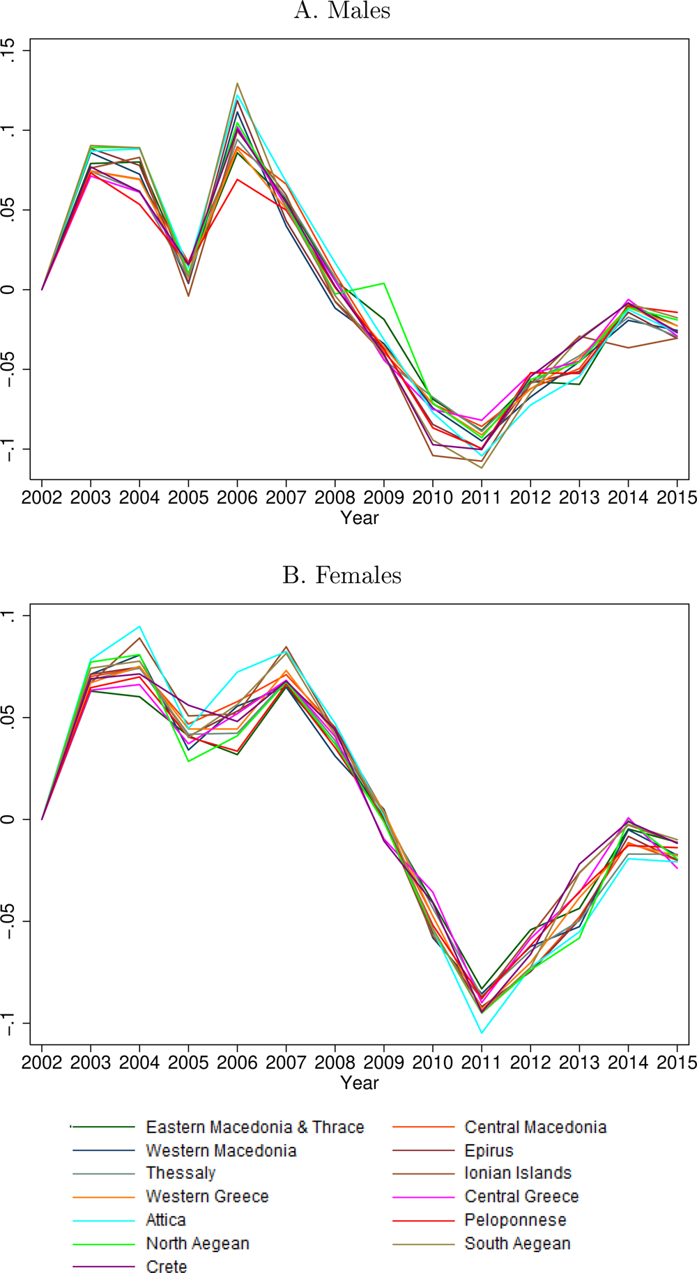
Figure A4. Predicted youth exposure to output shocks by region and year (shift-share instrument).


 Open access