


1. Introduction
Over the past few decades young people have become more and more educated in the Western world. At the same time, the share of young couples where both of the spouses are highly educated has been rising as well. It is theoretically possible that the latter trend in the prevalence of educational homogamy has been caused exclusively by the educational expansion: it is more probable that a person with a tertiary education degree marries another highly educated person if more individuals from the opposite sex obtain diplomas. However, other factors might have also played a role. For instance, the change in marital preferences from one generation to another is also a factor of natural suspect [see e.g., Kalmijn (Reference Kalmijn1998)].
In this paper, we investigate empirically the strength of various driving forces of young adults’ marriage patterns in the American society as well as in the societies of France, Hungary, Portugal, and Romania. In particular, we decompose the changes in the prevalence of educational homogamy between the late 1990s/early 2000s and early 2010s into three components. One component captures the ceteris paribus effect of changing educational composition of the population of young men and women.
The second component represents the effect of changing preferences in the absence of change in the educational distributions. This component is in the center of our interest because marital preferences in a society are informative about which groups are considered to be socially fitting [see Lichter and Qian (Reference Lichter and Qian2019)]. Since marital preferences cannot be observed directly, we identify them through their effects on the observable prevalence of homogamy.Footnote 1 Finally, the third component is the interaction term representing the effect of adjusting our preferences to the changes in the structural availability of partners with given traits.
In this paper, we contribute to the assortative mating literature by characterizing marital preferences with the reservation points of those individuals who form a couple, and also those who remain single. Our reservation points-based approach not only accounts for single people, but it accounts for them in a more sophisticated way compared to other papers in the literature. In particular, our approach distinguishes between “singles by choice” and “singles by chance”. Its advantage is that it leaves it even more to the empirical analysis to quantify the relative importance of preferences than those models do that account for only one type of singles.
We explain next with the examples of two hypothetical countries, how assumptions on singles relate to identifying changes in marital preferences. In these hypothetical countries there are two generations. It is also common across the countries that the prevalence of homogamy, as well as the share of single people, are higher in the younger generation, than in the older one.
In country A, those people in the old generation who have the highest education level and who did not mind to “marry down” are replaced by people in the new generation who have the same education level as their older peers, but have no desire to get married. This group of “singles by choice” in country A contributes to the increase in the prevalence of homogamy.
In country B, the population of men in the new generation is statistically the same as the population of men in the old generation: the share of men with any given education level is the same in the two generations; each man would like to marry a woman from his generation; and all men are indifferent about the education level of their spouses.
As to the women in country B, they are not completely the same in the two generations. Each woman in the old generation preferred to marry and could marry a man with the same education level as her own, or higher. The new generation of women is as “picky” as the old generation was: those women in the old generation who had a BA degree and who wanted to “marry up” are replaced by women in the new generation with the same marital preferences. However, all these women in the new generation have an MA degree. Unfortunately, many of them cannot find a spouse because there are only a few men with a PhD. These single women represent the “singles by chance” in country B, i.e., those who remain single even though they would like to be in a couple.
To sum, the prevalence of homogamy increases in both countries, however, for different reasons. In country A, it is the change in preferences that contribute to the increasing share of homogamous couples through the changes in the share of singles. By contrast, it is the change in the education levels that exerts the same effect in country B. These examples show that it is impossible to identify the causes of changing homogamy without estimating how the number of “singles by chance” and the number of “singles by choice” change.
In this paper, we tackle this identification problem in a novel way: we combine data from a dating site with census data to estimate the number of voluntary singles and the number of involuntary singles. The dating data are informative about the preferences of marriageable individuals, while the census reports the matching outcome, i.e., who is married to whom, who is cohabiting with whom, and who remained single. Our paper is not the first that uses dating data in the assortative mating literature.Footnote 2 However, we are not aware of any other study that uses dating data for the same purpose.
Out of the five countries analyzed, we have dating data only for one country. For this country, the outcome of the decomposition is qualitatively the same as the outcome of the decomposition obtained with an alternative approach.Footnote 3 The alternative approach is a statistical one based on the NM-method developed by Naszodi and Mendonca (Reference Naszodi and Mendonca2021).Footnote 4
The comparison of the outcomes goes beyond the scope of standard sensitivity analyses. It validates the statistical approach empirically, because any finding obtained on a rich set of data is commonly taken to be more credible. Therefore, our robustness analysis in section 5 deserves more attention than typical routinely performed robustness checks.Footnote 5
Before we validate the statistical approach in section 5, we use it in our benchmark analysis in section 4. Naszodi and Mendonca (Reference Naszodi and Mendonca2021) already applied this method for the US. Here, we extend the analysis for additional four countries. The multi-country nature of the benchmark analysis allows us to study whether some findings are specific to the US or common across several countries. So, our benchmark analysis is a replication of the analysis in Naszodi and Mendonca (Reference Naszodi and Mendonca2021). Our analysis is performed on census data from all those European countries, for which we could obtain good quality of linked educational attainment data of spouses from the Integrated Public Use Microdata Series (IPUMS) of the Minnesota Population Center.
Following Naszodi and Mendonca (Reference Naszodi and Mendonca2021), we measure the prevalence of homogamy by the proportion of couples in which the partners have the same education level.Footnote 6 This simple aggregate measure shows diverse dynamics in the five countries under study. It remained practically unchanged in the US and Hungary, it increased in France, whereas it decreased in Portugal, and Romania over the analyzed decade.
Interestingly, despite the divergence of these trends, we find that one of the factors driving the prevalence of homogamy has a universally positive trend: changing marital preferences over the spouses’ education level made the studied age group increasingly more inclined to match with others of similar educational traits after the turn of the Millennium in all the five countries. This finding is in line with the view that the social gap between different educational groups has substantially widened over the decade covering the Great Recession.
The rest of the paper is structured as follows. Subsection 1.1 reviews some selected papers in the assortative mating literature and it spells out the novelty of this paper relative to the reviewed papers. Section 2 defines the measures of homogamy used, while section 3 shows some stylized facts after describing our population data. Sections 4 and 5 present the decompositions obtained with the statistical approach, and the reservation points-based approach. Finally, section 6 concludes the paper.
1.1 Literature
This section highlights our contributions to two strands of literature. First, we contribute to studies examining the role of changing household formation on income inequality. Second, this paper joins to the camp of the growing literature that aims at identifying changes in marital preferences. We review some selected papers from both strands of literature (see Tables 1 and 2) and we discuss the connection between this paper and the studies reviewed.
Table 1. Comparing this paper with some selected papers on the consequences of changing marriage patterns

Notes: * DE, Germany; SOEP, Socio-Economic Panel; LFS, Labour Force Survey; DK, Denmark; NO, Norway; CPS, Current Population Survey. ** FR, France; HU, Hungary; PT, Portugal; RO, Romania.
Table 2. Comparing this paper with some selected papers on the causes of changing marriage patterns
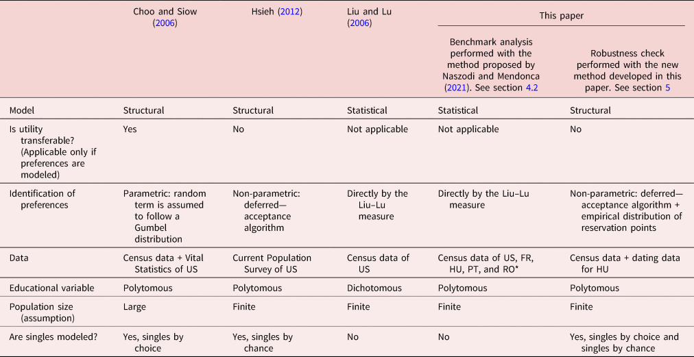
Notes: * FR, France; HU, Hungary; PT, Portugal; RO, Romania.
There is no consensus in the marriage-income inequality literature on the role of changing marriage patterns at forming inequality. In particular, the question is whether changes in the degree of educational assortative mating over the past decades had any effect on household income inequality. This is shown by the diverging findings in the papers by Eika et al. (Reference Eika, Mogstad and Zafar2019) and Dupuy and Weber (Reference Dupuy and Weber2018).
Eika et al. (Reference Eika, Mogstad and Zafar2019) present the striking finding that changes in homogamy hardly moved the time trend in household income inequality in the US between the early 1960s and the 2010s. While the other two factors considered by them, i.e., the increase over time in the income premiums for high school and college degrees (i.e., the economic returns to education) and the changes in the educational composition of the society, are found to account for a massive change in the household income inequality.Footnote 7
Some other studies in the literature present results that are qualitatively different from those in the Eika et al. (Reference Eika, Mogstad and Zafar2019) paper. For instance, Dupuy and Weber (Reference Dupuy and Weber2018) find that changes in the marital patterns can explain a sizable share (up to 1/3) of the observed increase in income inequality in the US between 1962 and 2017.
Dupuy and Weber (Reference Dupuy and Weber2018) explore what their approach deviates from those of Eika et al. (Reference Eika, Mogstad and Zafar2019), and how it causes the difference in the above findings. They argue that these qualitative findings hinge on whether single people are accounted for, or not. While dynamics in the number of singles are modeled explicitly by Dupuy and Weber (Reference Dupuy and Weber2018), singles are disregarded by Eika et al. (Reference Eika, Mogstad and Zafar2019) in their benchmark estimation (although not by their robustness check).
Our contributions relevant to the Eika et al. (Reference Eika, Mogstad and Zafar2019) and Dupuy and Weber (Reference Dupuy and Weber2018) papers are as follows. First, we find that the incorporation of singles in the analysis with our reservation points-based approach leads to the same qualitative result as with the statistical approach. The latter approach completely ignores the singles. This outcome of our robustness check is in line with the view of Eika et al. (Reference Eika, Mogstad and Zafar2019): disregarding singles does not necessarily influence our findings on the main drivers of inequality.
Second, we challenge the view that marital preferences over the partners education level would account for a large share of the increase in inequalities. Meanwhile, we do not question what is obvious. In particular, we do not question that changes in marital preferences can have significant effect on family formations. In fact, we find that in the analyzed five countries (US, France, Hungary, Portugal, and Romania) the share of educationally homogamous couples would have substantially increased after the turn of the Millennium provided only marital preferences had changed. Also, we do not question that the increasing share of educationally homogamous couples would contribute to the rise in inequality across dual-headed households.
What we do question though is that the identified changes in marital preferences would represent shocks that are exogenous in nature.Footnote 8 In fact, we form the hypothesis that marital preferences are shaped partly by the labor market. This hypothesis is supported by the co-movement of unemployment rates and preferences: when the employment prospects of people with a given education level improve relative to another educational group, they become relatively more attractive as partners. As it is shown by Figure 1, this relationship between the marriage market and the labor market is typically overlooked in the marriage–income inequality literature.

Figure 1. The channels connecting educational assortative mating, household income inequality, and some of their determinants. Notes: The straight, continuous arrows represent the channels examined in this paper by the decomposition exercise. The continuous curve indicates positive correlation that this paper provides evidence for by Figures 3 and 5, and also by Figure 6. The dashed arrows represent the channels investigated by the marriage–income inequality literature. Among the dashed arrows, the straight ones stand for the channels that are analyzed by Eika et al. (Reference Eika, Mogstad and Zafar2019) and Dupuy and Weber (Reference Dupuy and Weber2018) by their partial equilibrium approaches. While some general equilibrium analyzes, like the one by Fernandez et al. (Reference Fernandez, Guner and Knowles2005), model also the channels corresponding to the curved dashed arrows.
In this paper, we apply two approaches. One of them is the reservation points-based approach developed in this paper. It characterizes marital preferences at an aggregate level by the distributions of the reservation points. These distributions are allowed to be different for men and women, while also being education level-specific and generation-specific. The other one is the statistical approach developed by Naszodi and Mendonca (Reference Naszodi and Mendonca2021).
Our contributions to the literature with the reservation points-based approach and the statistical approach are equally important, although these contributions are of different types. The contribution with the reservation points-based approach is mainly theoretical since it validates the statistical approach. By contrast, the contribution with the statistical approach is mainly empirical because it sheds light on the common trend of marital preferences across the countries analyzed and the endogenous nature of these preferences.
Our reservation points-based approach builds on the insight of Dupuy and Weber (Reference Dupuy and Weber2018) that modeling the singles may be crucial. However, our approach is not the same as theirs. They use the Choo and Siow (Reference Choo and Siow2006) model that is from the family of models with one-type-singles, while our new approach accounts for two different types of single people: “singles by chance” and “singles by choice”. As we have shown in the introduction with the example of two hypothetical countries, working with a model with two-types-singles is pivotal at identifying the causes of changing homogamy and in particular, at identifying the directly unobservable changes in marital preferences. Therefore, our reservation points-based approach represents an important contribution to the literature.
Our reservation points-based approach shows some similarities to the model by Hsieh (Reference Hsieh2012). Most importantly, we use the aggregate version of the Gale and Shapley (Reference Gale and Shapley1962) algorithm proposed by Hsieh (Reference Hsieh2012) to derive the matching outcome from the distributions of reservation points. However, we deviate from the approach of Hsieh (Reference Hsieh2012) at least in two respects. First, Hsieh (Reference Hsieh2012) assumes that individuals are mutually acceptable for each other as partners. By contrast, we assume that women (men) with low education levels are not acceptable for those men (women) who have high reservation points. Second, an important novelty of our paper relative to Hsieh (Reference Hsieh2012) is that we use data from a dating site. These data allow us to observe the reservation points.
Next, we review some features of the statistical model. This model relies on the aggregate measure of marital preferences developed by Liu and Lu (Reference Liu and Lu2006) and generalized by Naszodi and Mendonca (Reference Naszodi and Mendonca2021). Whether the (generalized) Liu–Lu measure represents marital preferences well is not obvious.Footnote 9 Naszodi and Mendonca (Reference Naszodi and Mendonca2021) and Naszodi (Reference Naszodi2021c) provide empirical support for characterizing marital preferences at an aggregate level with the generalized Liu–Lu measure. They show that the variation of the Liu–Lu measure across certain generations is in line with the survey evidence from the Pew Research Center on Americans’ diverse views about spousal education. Moreover, Naszodi and Mendonca (Reference Naszodi and Mendonca2021) find that this is not the case with some alternative measures, such as the marital surplus matrix in Choo and Siow (Reference Choo and Siow2006), and the odds ratio matrix in Altham and Ferrie (Reference Altham and Ferrie2007), Breen and Salazar (Reference Breen and Salazar2005), Breen and Salazar (Reference Breen and Salazar2011), and Hu and Qian (Reference Hu and Qian2016).Footnote 10
This is a striking finding because, until now, these alternative measures enjoyed unbroken popularity among social scientists. The odds ratio has been commonly used to characterize preferences: for instance, when social scientists construct counterfactual contingency tables under unchanged marital preferences with the table transformation method of the Iterative Proportional Fitting (IPF) algorithm.Footnote 11 By applying the IPF (also called as the RAS algorithm), the odds ratio of the so-called seed table (i.e., the table to be transformed) is preserved. This is how the IPF supposed to keep marital preferences the same in the transformed table as in the seed table.
Naszodi and Mendonca (Reference Naszodi and Mendonca2021) present not only empirical arguments using survey evidence, but also several theoretical arguments to show that an alternative to the IPF, i.e., the transformation method developed by them, is more suitable for constructing counterfactual tables. Their method distinguishes itself from the popular methods not only by characterizing marital preferences with the matrix-valued generalized Liu–Lu measure, but also by its attractive analytical properties and the analytical properties of its transformed table. The transformed table is (i) unique, (ii) deterministic,Footnote 12 and (iii) given by a closed-form formula.Footnote 13
The transformation (i) commutes with the operation of merging categories,Footnote 14 (ii) works even if the seed table contains zeros,Footnote 15 (iii) can signal with a negative entry in the transformed table that the counterfactual scenario is not realistic.
As we will see, the robustness check in this paper provides additional supporting empirical evidence in favor of the Liu–Lu measure. Thereby, our robustness check contributes to the literature on selecting indicators for characterizing marital preferences at an aggregate level, and also for characterizing the dynamics of the social gaps.
2. The measures of “prevalence of homogamy” and “preference for homogamy”
This section relies on the work by Liu and Lu (Reference Liu and Lu2006) and Naszodi and Mendonca (Reference Naszodi and Mendonca2021). It introduces two types of measures of educational homogamy: (i) measures of “prevalence of homogamy” that characterize the equilibrium outcome of the search and matching mechanism in the marriage market; and (ii) measures of “preference for homogamy” capturing only one determinant of the equilibrium.
Throughout this paper, it is assumed that the educational trait is described by an ordered categorical variable that can take three possible values. Its value L stands for “low level of education” corresponding to not having completed the high school; M denotes “medium level of education” corresponding to having a high school degree, but neither a college degree nor a university degree; and H stands for “high level of education” corresponding to holding at least a BA diploma. Accordingly, there are 9 different types of marriages. The number of marriages of each type is captured by the contingency table:

where N m,f is the number of couples with husbands’ education level m ∈ {L, M, H} and wives’ education level f ∈ {L, M, H}. Once the contingency table B is known, the educational distributions of married men [N L,·, N M,·, N H,·] and women [N ·,L, N ·,M, N ·,H] are known as well.
2.1 The measures of “prevalence of homogamy”
Our education level-specific measure of prevalence of homogamy is the share of homogamous couples of a given type among all the couples: SHCa(B) = N a,a/N, where N a,a is the number of a, a type marriages with a ∈ {L, M, H}, while N denotes the total number of couples.
Our aggregate measure of prevalence of educational homogamy is the share of all types of homogamous couples among all the couples: $\rm {SHC}^{\rm {agg}}\it ( B) = {( N_{L, L} + N_{M, M} + N_{H, H}) }/{N}$ .
.
2.2 The measures of “preference for homogamy”
For the decomposition exercise, we need to construct the contingency table corresponding to the counterfactual that the marital preferences are from one period, while the educational distributions of women and men are measured in another period.
When we perform the benchmark decomposition using the statistical model, we characterize marital preferences by the generalized Liu–Lu measure. The generalized Liu–Lu measure is scalar valued, and equivalent to the original Liu–Lu measure proposed by Liu and Lu (Reference Liu and Lu2006) if the assorted trait is a dichotomous variable. For example, individuals can be either low educated (L) or high educated (H). If the assorted trait is dichotomous and represents an attractive characteristics (such as being highly educated), then the Liu–Lu measure is

where N H,H denotes the number of couples, where the spouses have high educational attainment; N H,· is the number of couples with high educated husbands; and N ·,H is the number of couples with high educated wives. While Q = N H,·N ·,H/N is the expected number of H,H-type couples under random matching. Furthermore, Q − is the biggest integer that is smaller than or equal to Q.
For an ordered trinomial assorted trait variable (i.e., an ordered categorical variable that can take three possible values) the generalized Liu–Lu measure is a matrix-valued measure. For its formula, see equation (1) in Appendix A in the online appendix (see https://doi.org/10.1017/dem.2022.21).
The Liu–Lu measure is invariant to a class of changes in the contingency table. We give a numerical example for a Liu–Lu invariant change with $K_0 = \left[ \matrix{ 925 & 125 \cr 75 & 375 }\right]$ and $K_1 = \left[\matrix{ 450 & 150 \cr 50 & 350 }\right]$
 , where $\rm {LL}( {\it K}_0) = {375 - ( {450 \times 500}/{1500}) \over \rm {min}( 450,\; \, 500 ) -( {450 \times 500}/{1500}) } = \rm {LL}( {\it K}_1) =$ ${350 - ( {400 \times 500}/{1000}) \over \rm {min}( 400,\; \, 500 ) - ( {400 \times 500}/{1000}) } = {3\over 4}$
 .
.
In this example, the share of high educated wives increased substantially from 1/3 = (125 + 375)/1500 to 1/2 = (150 + 350)/1000, while the share of high educated husbands increased only moderately from $30\% = ( 75 + 375) /1500$ to $40\% = ( 50 + 350) /1000$
 when the contingency table changed from K 0 to K 1. So, this example shows that the class of Liu–Lu invariant changes covers even asymmetric changes, i.e., where changes in the trait distribution of men and women are not the same.
Asymmetric changes are historically relevant, because we experienced them during the closure and the reversal of the educational gender inequality gap. Since the Liu–Lu statistics seems to be able to control for historically relevant changes in the educational distributions, it meets a necessary condition qualifying it to be interpreted as a measure of “preference for homogamy”.
It is important to highlight what the preferences in question, captured by the (generalized) Liu–Lu measure, are formed over. These preferences can be formed, in principle, not only over the partners’ education level but also over other characteristics, such as social status. This distinction is important. First, dissimilarity of preferences of two generations over the partners’ education level can be coupled with identical marital preferences of these generations over the partners’ social status provided a given educational attainment does not correspond to the same social status in the two generations. For example, obtaining a high school degree ensured higher status for our grandmothers than for us. “Like (grand)father like (grand)son”: young men today may have the same marital preferences as their grandfathers had, however, these stable preferences are probably formed over the social status of the potential wives and not over their education level.
This insight motivates an alternative interpretation of the changes in the (generalized) Liu–Lu measure over time: it signals changes in the social gap between people from different educational strata under the assumption of constant preferences over the partners’ social status.
3. Census data and stylized facts
This section describes the census data from two waves that are used for analyzing trends in homogamy in societies of France, Hungary, Portugal, Romania, and the United States. The first wave is from the late 1990s/early 2000s, and the second one is from the early 2010s. The data are from IPUMS.
Our data cover single people and heterosexual couples. The marital status variable in the census data has one common category: “married/in union”. Henceforth, we refer to both types of union as marriage.
The couples in our data are such that the age of the male partner is at least 25 years but strictly lower than 40 years. The motivation for choosing this age group for our analysis is threefold. First, many of those who are younger than 25 years have not completed their educational attainment. Second, marital preferences may change over the course of one's life. By studying a relatively narrow age group, we control for heterogeneity in preferences due to age. Third, for the sake of comparability, the census data used in the benchmark analysis cover the same age group as our dating data used in the robustness analysis. In order to work with a sufficiently high number of observations on the dating service users, we opt for a relatively broad definition of young adults.Footnote 16
Figure 2 allows us to compare both the educational distributions and the marital distributions across countries, over time, and also between the two genders. It reflects three well-known stylized facts. First, it documents the expansion of the education characterizing the analyzed decade: societies of the five countries in our sample were composed of more educated young men and women in the early 2010s than around 2000. Second, the traditional educational gender gap has not only been closed, but a new gap has started to open since women have already outperformed men in educational attainment in all the five countries by the early 2010s. Third, the proportion of singles has been drastically increased.
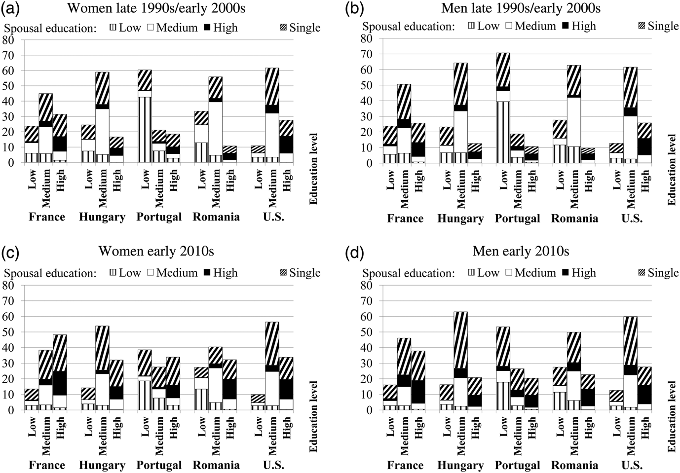
Figure 2. Educational and marital distribution of the population around the turn of the Millennium, and about the early 2010s (in %). Notes: Census data from IPUMS is used. The sample covers couples where the age of the male is between 25 and 40 and single individuals from the same age group. The earlier observations are from the years 1999 (France), 2001 (Hungary), 2001 (Portugal), 2002 (Romania), and 2000 (US). The latter observations are from 2011 for all the countries except the US, which is from 2010.
Next, we document trends in the prevalence of homogamy among couples. Table 3 reports how the education level-specific measures (i.e., the share of homogamous couples with specific educational attainment) and the aggregate measure (i.e., the share of all homogamous couples) have changed over the analyzed decade. What holds across all the countries is that the share of couples where both of the spouses have a diploma increased over time, as mentioned in the introduction of this paper. At the same time, the share of couples where neither of the spouses has a high school degree decreased in almost all the five countries. We reiterate our point made in the introduction: one cannot tell, simply on the basis of the above trends, whether they reflect only the effect of the general educational expansion or the effect of the changing marital preferences. This question is addressed in section 4.
Table 3. The proportion of the homogamous couples with different educational traits (in %)
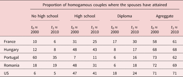
Notes: The same as below Figure 2, except that this sample covers only couples.
We emphasize that our benchmark analysis is performed by choosing couples to be the units of observation. Moreover, we make the following remarks. How the prevalence of homogamy relates to that of heterogamy is sensitive to the choice of the units of observation, i.e., whether those are couples or individuals. Homogamy is just the mirror image of heterogamy if these phenomena are captured by the share of homogamous couples and the share of heterogamous couples among all couples. But once we shift our focus from couples to individuals, the trend in heterogamy can be qualitatively different from the trend in homogamy with an opposite sign since not all individuals have a spouse (see Table 4).
Table 4. Prevalence of homogamy, heterogamy, and singlehood among individuals (in %)
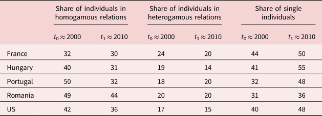
Notes: The same as below Figure 2.
Contrary to this sensitivity, we find robust evidence for the diverse trends in marriage patterns across countries over the analyzed decade: the increase in the prevalence of homogamy in France is supported not only by the increase in the share of homogamous couples (from 58% to 61%, see Table 3), but also by the decrease in the share of individuals in heterogamous relationship (from 24% to 20%, see Table 4). Similarly, the increasing prevalence of heterogamy in Portugal is supported not only by the substantial decrease in the share of homogamous couples (from 73% to 62%, see Table 3), but also by the increase in the share of individuals in heterogamous relationship (from 18% to 20%, see Table 4).
Finally, Figure 3 presents the dynamics of the diagonal elements in the Liu–Lu matrices over the analyzed decade. Its key message is that all the five countries under study shifted to the right and upward on it. This means two things. The social gap between people with high school degree and those without has widened after the turn of the Millennium universally. And also, the social gap between people with tertiary education diploma and those without has increased in all the five countries.
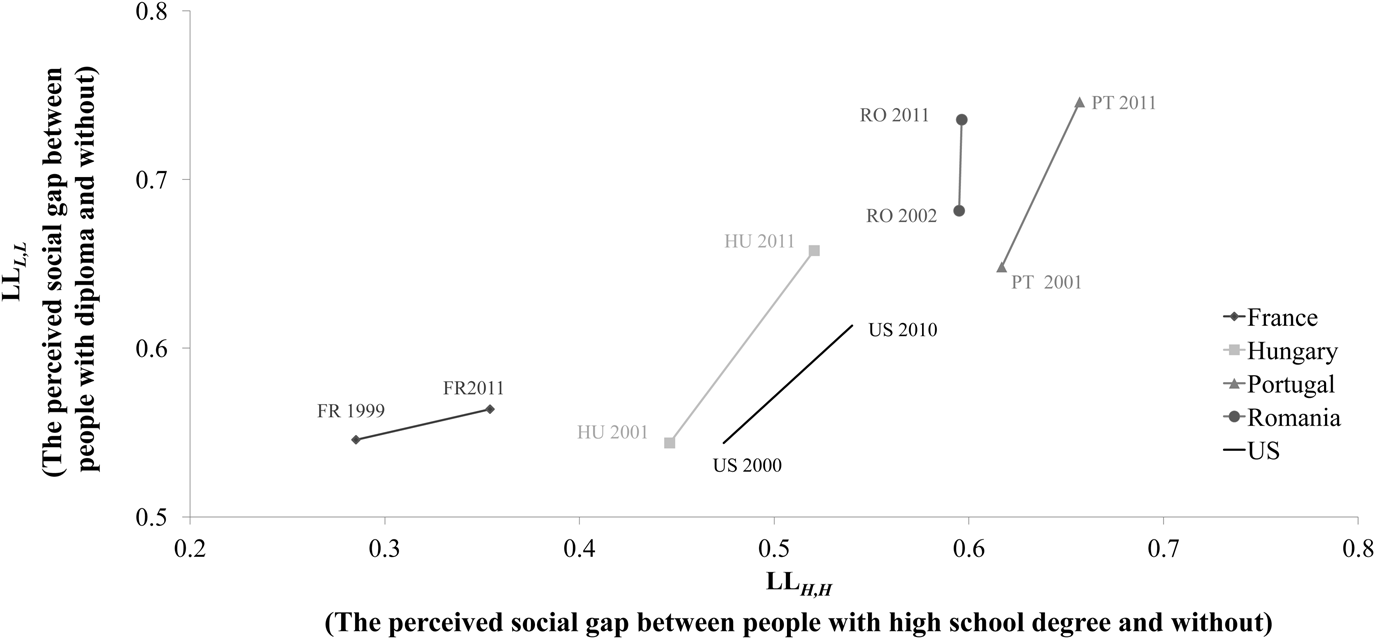
Figure 3. The dynamics of the diagonal elements in the Liu–Lu matrices.
It is challenging to judge directly the economic significance of the detected increases in the Liu–Lu measure. For instance, it is not obvious, whether its rise from 0.5 to 0.6 signals a “sharp increase” in preferences towards homogamy (and thereby, a drastic change in the stratification of the society) or not. This is because the Liu–Lu measure characterizes preferences for homogamy on an ordinal scale, not a cardinal one.Footnote 17 On the contrary, we can clearly feel the magnitude of the same change if it is observed in another measure, the share of homogamous couples.
To facilitate the interpretation of the observed changes in the generalized Liu–Lu measure, we perform a decomposition exercise in the next section. In particular, we project the changes in the prevalence of homogamy (measured on a cardinal scale) on the space spanned by the Liu–Lu matrix and the educational distributions. As a result of the decomposition/projection, we are able to tell how much would have the share of homogamous couples increased in each of the five countries if only their Liu–Lu matrices had changed but not the educational compositions.
4. Decomposing changes in the marriage patterns
This section describes the decomposition method used to net the effect of changing preferences from other drivers of marital patterns. Then, the outcome of the benchmark decomposition is presented before its robustness is checked.
4.1 Decomposition schemes
Some of the analyses in this paper are based on the decomposition scheme promoted by Biewen (Reference Biewen2014), while some others rely on the sequential decomposition scheme originally proposed by Oaxaca (Reference Oaxaca1973) and Blinder (Reference Blinder1973). The former scheme works as follows with two factors x and y observed in years t 0 and t 1; and a function f(x, y) mapping the space spanned by the two factors into ${\opf R}$ :
:

Whereas the original Oaxaca–Blinder decomposition scheme is either


depending on the assumed sequence of the changes in x and y.
By comparing the formula (3) with (4) and (5), one can see that the widely applied sequential decomposition scheme attributes the interaction effect (i.e., the last term in equation 3) either to the first factor, or to the second factor mistakenly. Unless this effect is negligible, the scheme in equation (3) is preferred to be used since the components estimated by this scheme do not depend on any arbitrary assumption about the sequence of changes in the factors; also, the ceteris paribus effects obtained with this scheme are not biased by the interaction effect. Following Biewen (Reference Biewen2012) and Biewen (Reference Biewen2014), we will refer to the scheme in equation (3) either as the path-independent decomposition scheme or the additive decomposition scheme with interaction effect.
In our specific setting of the benchmark analysis, function f tells us the share of homogamous couples. Factor x corresponds to the educational distributions, while y captures marital preferences with the Liu–Lu matrix. Time t 0 and t 1 correspond to census years nearest to 2000 and 2010, respectively.
The key step of our benchmark decomposition is to determine $f( x_{t_0},\; \, y_{t_1})$ and $f( x_{t_1},\; \, y_{t_0})$
 by constructing contingency tables under counterfactuals. For instance, determining $f( x_{t_0},\; \, y_{t_1})$
 requires to transform a contingency table (characterizing marital preferences in the census year close to 2010) into another contingency table in a Liu–Lu matrix invariant way by making the marginal distributions of the transformed table equal to its target marginals. The target marginals are from the census year close to 2000. A detailed description of the transformation method applied is provided by Naszodi and Mendonca (Reference Naszodi and Mendonca2021).Footnote 18
It is important to note that the additive decomposition scheme with interaction effect requires to model both of the counterfactual scenarios $( x_{t_0},\; \, y_{t_1})$ and $( x_{t_1},\; \, y_{t_0})$
 , while for the sequential decomposition it is sufficient to construct either one or the other. In the specific setting of our robustness check, we can estimate one of the factors, the marital preferences from the dating data from t 1 ≈ 2010, but not from t 0 ≈ 2000 due to not having such a rich set of dating data before 2010 as after that year. Therefore, the only analysis where we need to stick to the sequential scheme is the robustness check exploiting dating data.
4.2 Results of the benchmark decomposition
Figure 4(a) presents the outcome of the decompositions. It shows that the shifting preferences have exerted an economically significant positive effect on the share of homogamous young couples in all the five countries over the decade following the turn of the Millennium (see the dark bars in Figure 4(b)).

Figure 4. Decomposition of the change in the share of homogamous couples between the late 1990s/early 2000s and early 2010s. Notes: The earlier observations are from the years 1999 (France), 2001 (Hungary), 2001 (Portugal), 2002 (Romania), and 2000 (US). The later observations are from 2011 for all the countries except the US, which is from 2010. Changes in the aggregate and the education level-specific measures of prevalence of homogamy are decomposed by using the path-independent decomposition scheme presented by equation (3).
For instance, had the distribution of education levels of Americans remained the same as it was in 2000, the proportion of young homogamous couples would have risen from the already high value of 71% in 2000 to an even higher value of 75% by 2010.
When we interpret this finding, we keep in mind the following three points. First, interpreting the magnitude of this four percentage points increase in the share of educationally homogamous couples is definitely easier than interpreting the corresponding changes in the Liu–Lu matrix.
Second, this is an increase in a slowly changing variable capturing the difference in the share of homogamous couples between two overlapping generations. Some of those couples where the male partners were aged 35–40 in 2010 have already been formed and observed in 2000. The change in the share of homogamous couples among the newly-weds/new couples had to be even larger.
Third, throughout this section, we made the simplifying assumption that no factors played a role at shaping marriage patterns other than the considered two factors. However, changing matching mechanism or changing search frictions could be equally important as the changing composition of the studied age group with respect to its members’ marital preferences and education level [see McKinnish and Mansour (Reference McKinnish and Mansour2018)].
We consider our estimates on the effect of changing preferences to be conservative in the light of the fact that the search and matching mechanism has also changed. Most importantly, online dating became more popular over the studied period [see the left subfigure of Figure 1 in the paper by Rosenfeld and Thomas (Reference Rosenfeld and Thomas2012, p. 530)]. This new way of dating can connect people in the virtual space who would otherwise unlikely to meet in the physical space [see Ortega and Hergovich (Reference Ortega and Hergovich2017)]. So, the ceteris paribus effect of changing mating technology over the studied period is likely to be negative on the share of homogamous couples. Therefore, omitting the “search and matching technology-factor” makes our estimates on the considered factors downward biased.
4.2.1 Discussion of the results obtained with the benchmark decomposition
This section discusses some points made in this paper. For instance, it calls for an explanation why changing marital preferences are found to have a positive effect on the share of homogamous couples in all the five countries in our sample despite their cultural and demographic heterogeneity. Our suspect is the Great Recession representing a global shock to the national labor markets.
In particular, our hypothesis is that adverse and synchronized shocks to the labor markets during the global recession have changed marital preferences in the same way in many countries. Although we cannot formally test this hypothesis, we review some supporting evidences.
During the Great Recession, the unemployment rate was universally rising. The changing employment rate affected different educational groups differently regardless of their country of residence. As it is shown in Figure 5, people with higher education levels were universally more immune to the general job loss. For instance, in 2007, young American adults without upper secondary education had 15 percentage points less chance to be employed than their peers with average educational attainment. Relative to the same reference group, Americans with a tertiary education diploma had 7 percentage points more chance for having a job in 2007. By 2010, the former disadvantage grew by 2 percentage points, while the latter advantage increased by 3 percentage points.

Figure 5. The dynamics of the employment gaps (in %). Source: OECD: Educational attainment and labour-force status. Notes: The sample covers 25- to 34-year-old young individuals for the selected years of 2007 and 2010. Data are not available for Romania. The employment gaps are calculated as (i) the employment rate among young adults with tertiary education minus the average employment rate among young adults and (ii) the average employment rate among young adults minus the employment rate among young adults with below upper secondary education.
The shifts of countries to the right and upward on both Figures 3 and 5 demonstrate that there was a co-movement of the marriage market and the labor market in the 2000s.
Moreover, this co-movement can be documented not only with cross-sectional data on five countries, but also with time series data from the US: Figure 6 shows that Americans’ marital preferences monitored by surveys (with age-effect controlled for)Footnote 19 had a strong association with the employment gap between highly educated and low educated workers between 1990 and 2010 (see the solid black lines in Figure 6 whose correlation is as high as 0.74.).

Figure 6. The co-movement of Americans’ marital preferences and their labor opportunities. Source: Bureau of Labor Statistics; Labor Force Statistics; Pew Research Center. Notes: Survey respondents were asked to use the Likert scale to tell if they feel it is “very important”/…/“not at all important” for a good husband/wife/partner to be well-educated. In 2010, questions 23 and 24 in the Changing American Family survey were answered by 140 respondents from the age group 60–64 (representing early boomers); 167 respondents from the age group 50–54 (representing late boomers); 121 respondents from the age group 40–44 (representing early generation-X); 98 respondents from the age group 30-34 (representing late generation-X). In 2017, 612 respondents from the first age group answered the same questions in The American Trends Panel Wave 28 survey. We performed the age-adjustment by following Naszodi (Reference Naszodi2021c).
If decreasing relative labor demand for people with a given education level triggers diminishing relative “attractiveness” of these people on the marriage market then the documented co-movement reflects a causal relationship. In this case, the co-movement of the markets together with the global nature of the labor market shocks offer us a potential explanation for the qualitatively common trend in marital preferences across the analyzed countries.
Our findings can be linked to the household formation–income inequality literature. In this literature there is no agreement over the role of marital preferences at shaping household earnings inequality over the past decades. In abstracto, the debate centers around whether the marriage market is mostly the source of certain shocks or rather it acts mainly as a shock amplifier.
This debate has relevance for policy-making: if a phenomenon can be attributed largely to a secular factor, then there is only limited scope for any intervention. By contrast, if family formation significantly influences income inequality across households while the increasing segmentation of the marriage markets is largely due to adverse processes on the educational market or the labor market, then policies affecting these markets might have the potential to mitigate income inequality even indirectly via changing the marriage patterns.
The empirical evidences reviewed in this paper are more in favor of the second view: we find that changes in marital preferences are unlikely to be due to exogenous preference shocks since those correlate with changes in the labor markets. At the same time changing preferences seem to have a non-negligible effect on the aggregate prevalence of homogamy in the countries studied.
Finally, we make some points relevant for the empirical identification of how marital preferences affect income inequality. The effects of marital preferences on the education level-specific homogamy measures (dark bars in Figure 4(b)) are dwarfed next to the effects of educational distributions (white bars in Figure 4(b)). However, this is not the case for the same effects once being presented in a more meaningful way as aggregates over the three education levels (see Figures 4(a)). The small but positive education level-specific effects of marital preferences gain economic significance by being add up. While the education level-specific effects of the educational distribution with varying sings counterbalance each other to some extent when being aggregated. This comparison shows that the choice of metric used for characterizing prevalence of homogamy (education-level specific vs. aggregate) is not innocuous: if the effect of marital preferences on household formation is obscured, so is its effect on income inequality.
Similarly, the choice of the decomposition scheme does not seem to be neutral either. For instance, if the marital preferences had remained stable over time in France, the proportion of homogamous couples would have risen by one percentage points between 1999 and 2011 according to the additive decomposition with interaction effect presented by Figure 4(a). By contrast, the sequential decomposition could falsely suggest that the same effect is negligible (=1–1) when it arbitrarily attributes the joint effect of shifting preferences and changing educational distributions to the changing educational composition.Footnote 20
5. Robustness check
This section presents an analysis for checking (i) whether the Liu–Lu measure captures the effect of changing preferences sufficiently well and (ii) whether accounting for singles with our reservation points-based approach can modify our key finding.Footnote 21
The motivation for the robustness check is twofold. First, there was a universal increase in the share of single people: it increased at least by 5 percentage points among the 25–40 years old people in all the analyzed countries over such a short period as a decade (see Table 4). While this dynamics can be taken into account by our reservation points-based approach, it is disregarded by the statistical approach applied in our benchmark analysis.
Second, a certain share of the single people is likely to be involuntary singles, i.e., people who would like to be in a couple but are not. When imposing the simplifying assumption that these people keep themselves away from the marriage market, as we did so implicitly in the benchmark analysis, we might get biased components.
All these call for checking whether our results obtained by the benchmark analysis are robust to the way preferences are captured. To meet this goal we employ the reservation points-based approach utilizing direct observations on marital preferences from a dating site.
The rest of this section is structured as follows. Subsection 5.1 presents how the equilibrium in the marriage market is determined with the reservation points-based approach as a function of the marital preferences and the educational distributions. Subsection 5.2 briefly introduces the data from the dating site. Subsection 5.3 describes how the preferences characterizing the population is estimated from the observed preferences of the dating site users and the gender-specific educational distributions of the Hungarian population of young adults. It also offers a supplementary analysis for checking the representativity of the sample of dating service users. Subsection 5.4 presents the outcome of the decomposition obtained with the reservation points-based model and the dating data.
5.1 Matching model
In our model, individuals are assumed to have only two characteristics relevant for matching.Footnote 22 One of the characteristics is the educational attainment. The other characteristic is the reservation point of an individual, which is the minimum educational attainment of an acceptable partner for the person.
The intuition behind our parsimonious two-variable framework is the following. A number of characteristics that are generally viewed to be relevant for matches in reality (including health, wealth, beauty, intelligence) are likely to be well represented by the reservation points of individuals. For instance, if someone perceives herself (himself) to be a strong candidate due to her (his) characteristics that a potential partner is expected to appreciate, then it is reflected in her (his) high reservation point.
In the empirical application of the model, we distinguish between 12 different types of men and 12 different types of women since we consider three education levels, and four reservation points. The distribution of women and men in the population is given by the following tables:

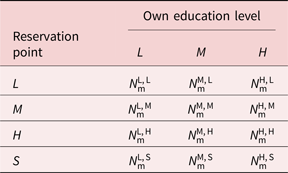
where $N_{\rm {w}}^{{\rm {OE}}, \, {\rm {RP}}}$ ($N_{\rm {m}}^{{\rm {OE}}, \, {\rm {RP}}}$
 ) denote the number of women (men) in the population with own education level OE ∈ {L, M, H}, and reservation point RP ∈ {L, M, H, S}. Individuals with reservation point RP = S are the voluntarily singles, who do not want to be in a couple.
Similar to Hsieh (Reference Hsieh2012), we assume that preferences are formed over characteristics, and not over individuals. The preference lists are assumed to be based on an lexicographical ordering of the two characteristics. In particular, everybody finds potential partners with higher education level to be more attractive. Among potential partners with the same education level those are found to be more attractive, who have higher reservation points. So, the preference list of each man and each woman with reservation point L is:
${HH} \succ {HM} \succ {HL}\succ {MH} \succ {MM} \succ {ML}\succ {LH} \succ {LM} \succ {LL} \succ \rm {remaining} \; \rm {single}$ . As before, the first characteristic is the own education of the potential partners from the opposite sex, while the second characteristic is their reservation point.
Similarly, the preference list of individuals with reservation point M is ${HH} \succ {HM} \succ {HL}\succ {MH} \succ {MM} \succ {ML}\succ { \rm remaining\; single} \succ {LH} \succ {LM} \succ {LL}$ ; and the preference list of those with reservation point H is ${HH} \succ {HM} \succ {HL}\succ$ ${\rm remaining \;single} \succ {MH} \succ {MM} \succ {ML} \succ {LH} \succ {LM} \succ {LL}$
 . Finally, for those individuals with reservation point RP = S, remaining single dominates marriage (even to a HH-type person).
Once we know the preferences and characteristics of each individual, a matching algorithm, such as the Gale–Shapley deferred-acceptance algorithm, can provide us with the matching outcome. The key idea of the Gale–Shapley algorithm is that men make proposals to women, and women accept or decline these offers. The algorithm can also be used with swapped roles. However, the first approaches initiated by the males in our dating data are more common than those initiated by females. So, we will introduce and apply that version of the algorithm where the men make proposals and not the women.
Obviously, voluntary singles do not make offers and do not receive offers. So, they do not have any role in the Gale–Shapley algorithm. Hsieh (Reference Hsieh2012) describes the Gale–Shapley algorithm as follows: “In the first round, each man [if not a voluntary single] makes an offer to his most preferred woman. The women then collect offers from the men, rank the men who made proposals to them, and keep the highest ranked men engaged. The offers from the other men are rejected. In the second round, those men who are not currently engaged make offers to the women who are next highest on their list. Again, women consider all men who made them proposals, including the currently engaged man, and keep the highest ranked man among these. In each subsequent round, those men who are not engaged make an offer to the highest ranked woman who they have not previously made an offer to, and women engage the highest ranked man among all currently available partners. The algorithm ends after a finite number of rounds.”
In this paper, we use the so-called modified Gale–Shapley algorithm proposed by Hsieh (Reference Hsieh2012).Footnote 23 It assumes the matching algorithm to be the same deterministic algorithm as the original Gale–Shapley algorithm described above. However, it provides us with only aggregate statistics about the matching outcome, i.e., the educational distribution of couples and involuntary singles. Since it does not aim at determining who will be matched with whom (and who remain single), this algorithm is faster than the original Gale–Shapley algorithm.
We illustrate the functioning of the modified algorithm by a numerical example. Suppose that our focus is on one segment of the marriage market: we would like to know the number of couples N H,H where both spouses have a university diploma. Further, suppose that the relevant input variables take the following values: $N_{\rm {w}}^{{\rm {H}}, \, {\rm {H}}} = 36$ , $N_{\rm {w}}^{{\rm {H}}, \, {\rm {M}}} = 63$
 , $N_{\rm {w}}^{{\rm {H}}, \, {\rm {L}}} = 2$
 , $N_{\rm {m}}^{{\rm {H}}, \, {\rm {H}}} = 31$
 , $N_{\rm {m}}^{{\rm {H}}, \, {\rm {M}}} = 60$
 , and $N_{\rm {m}}^{{\rm {H}}, \, {\rm {L}}} = 9$
 .
.
In the first step of the algorithm, all men make proposals to the 36 HH-type women (who have high level of educational attainment and high reservation point). All 36 HH-type women accept a proposal, out of which 31 is made by HH-type men and 5 is made by HM-type men. Next, all men who are not engaged currently make a proposal to the 63 HM-type women. All 63 HM-type women accept a proposal, out of which 55 is made by HM-type men and 8 is made by HL-type men.
Finally, the last unmatched high educated man makes a successful proposal to one of the 2 HL-type women not engaged currently. (The other HL-type women will be matched with a men with education level M or L if there are such men in the population with RP ≠ S. Otherwise, she will stay single involuntarily.) In this numerical example N HH is calculated by simply adding up 36, 63, and 1. Determining other points of the educational distribution of couples works analogously.
5.2 Dating data
The source of our dating data is a Hungarian online dating service provider. Its dating site is one of the most popular sites among Hungarian speaking users. The examined market is the matchmaking segment, i.e., we restrict our analysis to those users whose indicated reason for joining the service is to find a partner for a long-term/serious relationship.Footnote 24 Our data cover the population of users who signed up for the dating service in a given year, in 2017.
In order to make our second decomposition comparable with the benchmark decomposition, we restrict the data to those men who are strictly older than 24 years, but strictly younger than 40 and those women who look for a partner in this age range. In addition, we restrict the sample to those users, who indicate their own educational attainments and their search criteria regarding the education level of the desired partner. The number of users in this final sample is 735, out of which 355 are women and 380 are men.
We use only aggregated data from the dating site represented by Figure 7, i.e., the distributions of the search criteria conditional on the users’ gender and educational attainment. This figure supports two points. First, female users tend to set higher education levels as their search criteria than males with the same educational attainment.Footnote 25 Second, the dating site users with a given educational attainment tend to be more picky than their peers with lower qualification level.

Figure 7. Distribution of the search criteria of the online dating service users conditional on their gender and educational attainment. Source: The data are from a Hungarian dating site. Notes: The search criteria of the users are for the desired partners’ education levels. Those are interpreted as being the reservation points. Male users in our sample are aged between 25 and 40 years, while female users in the sample look for a partner in this age range.
Unlike us, the dating site users can observe neither each other's search criteria, nor the distribution of the search criteria. By contrast, they can observe many characteristics of each other that the econometricians cannot or would not.
We assume that the search criteria of the Hungarian dating site users are identical to their reservation points. In principle, one's search criterion can be anything between one's reservation point and aspiration point (i.e., the highest educational attainment of those who the person can hope to be matched with). However, if the market is as thin as the Hungarian marriage market, it seems plausible to interpret the search criteria as reservation points.
5.3 Estimation of the distribution of unobserved types and a supplementary analysis
We apply a fairly standard approach for estimating the number of individuals in the population with a given gender, education level, reservation point (if not S), and marital status from the number of users of the dating site with the same gender, education level, and reservation point. In this approach, we combine the maximum likelihood estimator and the generalized method of moments estimator (GMM) as it is described in Appendix B in the online appendix (see https://doi.org/10.1017/dem.2022.21).Footnote 26
Our approach relies on the assumption that the distribution of the search criteria set by the users in our sample with a given education level and gender are representative to the distribution of the reservation points of young Hungarian adults, other than voluntary singles, with the same education level and gender.Footnote 27
The following supplementary analysis investigates the plausibility of this assumption. It exploits the fact that there are moment conditions on the distribution of couples that are not used by the GMM estimator (see Appendix B in the online appendix). We compare the model-implied values of these moment conditions with their population counterparts: the education level-specific measure of homogamy calculated from the model-based contingency table are contrasted with the observed education level-specific measure of homogamy. Figure 8 shows that the corresponding numbers are very close to each other. This finding dispels the doubt not only concerning the representative nature of the dating data but also concerning the adequacy of the Gale–Shapley matching algorithm.

Figure 8. Validation of the model by comparing moments that are not matched by the GMM. Source: Authors’ calculations using census data from 2011 and aggregate data from a Hungarian dating site presented by Figure 7. The moment conditions used by the GMM do not cover the following three conditions: SHCL* = SHCL, SHCM* = SHCM, SHCH* = SHCH (see the Appendix).
5.4 Decomposition using dating data
This section presents the results performed with the decomposition method exploiting dating data and census data. We show the outcome of the decompositions obtained with the sequential decomposition scheme in equation (5), where preferences change first, and the educational distributions change second.
Any other decomposition either cannot be performed due to data limitations, or its estimates are not directly comparable with those resulted from the benchmark decomposition. For instance, since our dating data are from t 1 = 2010s (and not from t 0 = 2000s), we can use neither the decomposition scheme in equation (3), nor the sequential decomposition scheme, where the factors change in the reversed sequence.
The sequential decomposition scheme in equation (5) (i.e., where preferences change first) attributes the joint effect of the factors fully to the changing educational distributions. Thereby, it results in a biased estimate on the effect of this factor, while the same source of bias does not affect the other factor. Fortunately, the factor that is in the center of our interest is this bias-free second factor, i.e., the preferences.
Throughout this section, what we mean under unchanged preferences in the society is that the type-specific and gender-specific distribution of the reservation points (including the type-specific and gender-specific distributions of voluntary singles) are kept fixed. So, factor y in equation (5) is the set of distributions of the reservation points.
Our robustness check confirms the main finding of the benchmark decomposition: the changes in the marital preferences over the partners’ education levels and getting married at all made educational homogamy more prevalent. This is apparent from the aggregate results presented by Figure 9, where the dark bar is in the positive range.

Figure 9. Decomposition of the changes in the share of homogamous couples with a specific education level and the share of all educationally homogamous couples between 2001 and 2011 in Hungary. Notes: The decomposition uses census data for Hungary from 2001 and 2011 in combination with the dating data. Changes in the aggregate and the education level-specific measures of prevalence of homogamy are decomposed by the Oaxaca–Blinder decomposition scheme. It works as follows with factors being preferences (determined by the estimates for $P^{\rm {RP} \neq S}$ and $P^{\rm {RP} = S}$
 ) and availability of potential partners with given education levels (determined by the gender-specific educational distributions) and observations from time 0 and 1:$f( a_1,\; \, p_1) -f( a_0,\; \, p_0) = \overbrace {f^\ast ( a_0,\; \, p_1) -f( a_0,\; \, p_0) }^{\rm {due\ to\ } \Delta\ \rm {preferences}} + \overbrace {f( a_1,\; \, p_1) -f^\ast ( a_0,\; \, p_1) }^{\rm {due\ to\ } \Delta\ \rm {availability\ ( edu.\ distr.) }}$
 , where function f takes the observed value of a given homogamy measure, function $f^\ast$
 does the same but under a counterfactual constructed by the modified Gale–Shapley deferred-acceptance algorithm. Finally, the effect of changing preferences is decomposed as, ${f^\ast ( a_0,\; \, p_1) -f( a_0,\; \, p_0) } = \overbrace {f^\ast [ a_0,\; \, p( \widehat {P}^{\rm {RP} \neq S}_1 , \ \widehat {P}^{\rm {RP} = S}_0 ) ] -f[ a_0,\; \, p( \widehat {P}^{\rm {RP} \neq S}_0,\; \, \widehat {P}^{\rm {RP} = S}_0 ) ] }^{\rm {due\ to\ } \Delta\ \rm {distribution\ of\ reservation\ points\ of\ those\ who\ would\ like\ to\ be\ matched}} +$ $\underbrace {f^\ast [ a_0,\; \, p( \widehat {P}^{\rm {RP} \neq S}_1,\; \, \widehat {P}^{\rm {RP} = S}_1 ) ] -f^\ast [ a_0,\; \, p( \widehat {P}^{\rm {RP} \neq S}_1,\; \, \widehat {P}^{\rm {RP} = S}_0 ) ] }_{\rm {due\ to\ } \Delta\ \rm {share\ of\ the\ voluntary\ singles}}$
 .
.
We make two general points relevant for model selection. First, the investigated total effect of the changing preferences is quantified to be of the same magnitude by our benchmark decomposition as by this robustness analysis: Figures 4(a) and 9 report the effect to be five and four percentage points, respectively. This suggests that the identified effect of marital preferences is not particularly sensitive to whether both the voluntary and the involuntary single people are modeled or neither.
Second, if one disregarded the kind of adjustment along the extensive margin that is due to the changing share of the voluntary singles, then the above four percentage points effect would be estimated to be negligible (see the hardly visible striped bar in Figure 9 corresponding to the aggregate value).
The second point confirms the view shared by Dupuy and Weber (Reference Dupuy and Weber2018) that assuming away adjustment along the extensive margin might bias the estimates of the marital preference-effect. Whereas the first point demonstrates that the size of the bias can be small if the model is flexible enough to attribute the adjustment along the extensive margin not only to the changing preferences but also to the changing educational distributions.
6. Conclusion
In this paper, we developed a method for decomposing observed changes in the marriage patterns with the aim of quantifying the effect of shifting marital preferences on household formation. The distinctive feature of the new method relative to some other methods in the literature is that it is able to account for single people in an elaborated way by distinguishing between voluntary singles and involuntary singles. The new method served for checking the robustness of our benchmark decomposition.
For the benchmark analysis, we applied a statistical method which, unlike the new method, completely disregards the possibility that individuals can remain single. We used this statistical method for studying the American, French, Hungarian, Portuguese, and Romanian marriage markets by exploiting census data on the education level of young couples from around the Millennium and about 2010. Specifically, we decomposed the changes in the proportion of educationally homogamous young couples over the analyzed decade into the effects due to the changing composition of the studied age group with respect to its members’ marital preferences and qualification level and the joint inseparable effect of both types of changes.
The main finding obtained with our benchmark decomposition is that one of the considered factors made young adults increasingly more inclined to match with others of similar educational traits over the analyzed decade in all the five countries. Changes in this factor can be interpreted either as the changes in marital/mating preferences over the partners’ education level, or, alternatively, as the widening of the social gap between people from different educational strata. The latter interpretation is favored provided that marital preferences are stable and formed over the partners’ social status for which education level is just an imperfect proxy.
Neither the marital preferences, nor the social gaps are directly observable. Still, we could cross-check our findings about these unobservable phenomena with an observable phenomenon: we presented evidence for the changes in the marriage market and the labor market in the studied countries suggesting the simultaneous appreciation of credentials on both markets over a period covering the Great Recession.
Although this correlation across different markets is in line with our intuition, some of our other findings might be found surprising. For instance, it can be deemed to be even counterintuitive by those who would study the stratification of societies through the changing marriage patterns without performing any decomposition exercise. This is because the identified general closure of the analyzed societies along the educational dimension is far not apparent from the dynamics of certain raw measures: e.g., the proportion of educationally homogamous couples even decreased in Portugal and Romania after the turn of the Millennium.
Finally, we found the identified effect of changing preferences in Hungary between 2001 and 2011 to be robust to whether both “singles by choice” and “singles by chance” are modeled or neither. This finding questions the view that failing to model the possibility of remaining single necessarily results in a substantial underestimation of the effect of changing mating preferences. One direction of future research is the replication of our robustness analysis for other countries and periods.
Supplementary material
The online appendix of this article can be found at https://doi.org/10.1017/dem.2022.21, while the code and data used are available at http://dx.doi.org/10.17632/fxdgzctpfj.1.
Acknowledgments
The authors are grateful to Gergely László for providing them aggregate dating data. Also, the authors thank Pierre-André Chiappori, Alfred Galichon, and Erik Plug for the helpful discussions and acknowledge comments from Vera Alpár, Andrea Barta, Liliana Cuccu, Sven Langedijk, Magne Mogstad, Eszter Naszódi, Tamás K. Papp, Sylke Schnepf, András Simonovits, Kornél Steiger, Iván Szelényi, Márta Ujvári, Stefano Verzillo, and two anonymous reviewers.
Author contributions
Anna Naszodi formed the concept of the research and wrote the first draft of the manuscript; positioned the paper within the literature; collected data from IPUMS, the Pew Research Center, and a Hungarian dating site. Finally, she revised the paper by incorporating comments from the anonymous reviewers. Francisco Mendonca made some first-round analysis of the census data. He implemented the new method using dating data in R. Also, he contributed by proof reading the manuscript and formatting its tables. In addition, he contributed indirectly by working on two companion papers entitled “A new method for identifying the role of marital preferences at shaping marriage patterns” and “A new method for identifying what Cupid's invisible hand is doing”. Both authors have read and approved the final manuscript.
Competing interests
None.
Disclaimer
The views expressed in this paper are those of the authors and do not necessarily reflect the official views of the European Commission.


 Open access