3.1 Base values

The starting point for estimating values for low- and middle-income countries is often either values developed for use in national U.S. regulatory analyses or for application by OECD member countries. These estimates were derived at different times using differing approaches, but are each based on substantial review and evaluation of a large number of studies and are well established and widely used. In recent work, Viscusi and Masterman have suggested instead relying on a meta-analysis of U.S. wage-risk studies, which results in estimates within the same range as those applied by the U.S. regulatory agencies.

U.S. regulatory agencies typically develop their recommendations by reviewing the literature and identifying a range of values and a central estimate from selected studies (U.S. Environmental Protection Agency, 2010a ; U.S. Department of Health and Human Services, 2016; U.S. Department of Transportation, 2016). Each agency uses different criteria and includes different studies in developing their estimates, but all rely primarily on wage-risk studies. The OECD has taken a different approach, focusing on stated-preference studies conducted globally and using meta-analysis to combine the results (OECD, 2012).

Comparing the monetary values requires translating them into the same currency for the same year. Rather than making this conversion, we compare the ratio of the reported values to gross national income (GNI) per capita for the country, in the same year as the VSL estimate.Footnote ⁴ Although many different income measures could be used (see Hammitt, Reference Hammitt2017), we rely on GNI per capita because consistently-derived estimates are available and easily accessible for a large number of countries, and because it is a broader measure than gross domestic product (GDP) per capita.

To translate values across currencies, we use purchasing power parity. Purchasing power parity is an index designed to represent what money can purchase in different economies. Compared with market-exchange rates, it better reflects the resources available to the population of each country when considering how these resources may be allocated across achieving mortality risk reductions and consuming other goods and services. One international dollar would buy a comparable quantity of goods and services in the country of concern as would a U.S. dollar spent in the United States. This means that U.S. GNI per capita is the same regardless of whether it is expressed in U.S. or international dollars.

Table 1 provides the estimates used by U.S. agencies and the OECD, expressed both as VSL and as WTP for a small risk change and compared to GNI per capita. The relationships between the U.S. values and income are similar across the three agencies; the relationship of the OECD estimate to income differs significantly.

Table 1 Comparison of VSL to GNI per capita: U.S. and OECD.

USEPA  $=$  U.S. Environmental Protection Agency USDHHS  $=$  U.S. Department of Health and Human Services USDOT  $=$  U.S. Department of Transportation Note: The U.S. estimates are designed to address nationwide policies; the OECD estimate is intended for application to analyses that address all OECD countries. GNI per capita is reported for the same year as the estimate.

These recommended values change periodically as new studies are completed and researchers develop new insights into best practices. For example, the U.S. Environmental Protection Agency (USEPA) has proposed to update its estimates based on meta-analysis of selected studies and advice from its expert panels (U.S. Environmental Protection Agency, 2016; Khanna et al., Reference Khanna2017). In addition, researchers are now updating the database and meta-analysis that underlies the OECD estimates.Footnote ⁵

Recently, Viscusi and Masterman recommended instead relying on meta-analysis of wage-risk studies that use data from the U.S. Census of Fatal Occupation Injuries (CFOI) (Viscusi, Reference Viscusi2015b ; Viscusi & Masterman, Reference Viscusi and Masterman2017a ,Reference Viscusi and Masterman b ; Masterman & Viscusi, Reference Masterman and Viscusi2018; Viscusi, Reference Viscusi2018).Footnote ⁶ In this research, Viscusi and Masterman assess the effects of publication-selection bias, which occurs when researchers or journals reject estimates that fall outside of a range deemed acceptable. They find substantial evidence of such bias both in U.S. studies that rely on other sources of risk data and in datasets that include international sets of revealed- or stated-preference studies. Their recommended base estimate, derived from meta-analysis of U.S. studies that rely on CFOI data, is a VSL of $9.6 million in 2015 U.S. dollars.

This U.S. estimate is very similar to the values currently used by U.S. regulatory agencies. If we update the values in Table 1 to 2015 dollars, using the approaches for adjusting for inflation and real income growth followed by each organization, the U.S. central estimates are all between $9 million and $10 million. The OECD estimate for 2015 is much lower; about $4 million. While GNI per capita is higher in the U.S. than across the OECD countries, the effect of income alone is likely to be smaller than implied by the large difference between the estimates. The difference is also attributable to the divergent approaches used to select studies and combine the results.

3.2 Adjustment for income differences

When applying these estimates in other settings, a key question is the extent to which they should be adjusted for variations in the risks and populations affected. The consensus in the reviews and guidance documents referenced above is that the available evidence is not sufficient to support adjustment for most differences. The one exception is income. Many, if not most, guidance documents and other reviews suggest that these estimates should be adjusted for differences in population-average income across countries and over time.Footnote ^{7 ,} Footnote ⁸

Because these values represent the trade-off between spending on mortality risk reductions and spending on other things, it would be nonsensical to expect that the values would be the same for individuals with substantially different income levels. For example, as illustrated in Table 1, the U.S. VSL estimates suggest the average U.S. resident is willing to pay amounts approaching $1000 dollars for a 1 in 10,000 mortality risk change, equivalent to about 1.6 to 1.7 percent of GNI per capita. In lower-income countries, this sum would represent much or all of an individual’s yearly income.Footnote ⁹ It seems implausible or impossible that an average individual in these countries would be willing to spend such a large sum on such a small risk reduction, given other essential needs. Overall, individual WTP per unit of risk reduction is expected to decrease as income decreases, resulting in a smaller VSL.

To extrapolate values across countries, analysts select an estimate (or estimates) of the degree of change in the VSL associated with a change in income; i.e., the VSL income elasticity. Although comparisons among high-income populations often find that changes in the VSL are less than proportional to changes in income (an income elasticity of less than one), comparisons between populations with large income differences often find that changes in the VSL are more than proportional to changes in income (an income elasticity of greater than one). An income elasticity greater than one implies that the ratio of VSL to GNI per capita is smaller in lower- than in higher-income populations. This seems reasonable given that lower-income individuals must devote a larger share of their incomes to necessary or urgent expenses.

Adjusting a base VSL for income differences requires an income estimate for the population to which the base VSL applies, an income estimate for the target population, and an estimate of the rate at which VSL changes as income changes; i.e., the average elasticity over the relevant income range. The formula is:

(1) $$\begin{eqnarray}\text{VSL}_{\text{target}}=\text{VSL}_{\text{base}^{\ast }}(\text{Income}_{\text{target}}/\text{Income}_{\text{base}})^{\text{elasticity}}.\end{eqnarray}$$

It is often convenient to work with ratios of VSL to income rather than VSL itself. This is in part because working with ratios avoids the need to convert values to a common year.Footnote ¹⁰ Some also find ratios easier to understand and apply. Derived from the equation above, the relationship of the ratios is:

(2) $$\begin{eqnarray}\displaystyle & & \displaystyle (\text{VSL}_{\text{target}}/\text{Income}_{\text{target}})=\nonumber\\ \displaystyle & & \displaystyle \quad (\text{VSL}_{\text{base}}/\text{Income}_{\text{base}})^{\ast }(\text{Income}_{\text{target}}/\text{Income}_{\text{base}})^{(\text{elasticity}-1)}.\end{eqnarray}$$

The same formulas can be used to extrapolate these values over time within the same country. In that case, the base VSL and income level are for the starting year, and the target VSL and income level are for a future year. Commonly, analysts assume that the same elasticity estimates apply over time as across different populations at the same point in time.Footnote ¹¹

Changes in the income elasticity can change the results by orders of magnitude. Hammitt and Robinson (Reference Hammitt and Robinson2011) report that the then-existing studies found VSL income elasticities ranging from as low as 0.1 to greater than 2.0. More recent reviews seem to be coalescing around estimates closer to 1.0 (OECD, 2016; World Bank and IHME, 2016; Viscusi & Masterman, Reference Viscusi and Masterman2017a ,Reference Viscusi and Masterman b ; Masterman & Viscusi, Reference Masterman and Viscusi2018), generally recommending elasticities around 0.8 for extrapolating across high-income countries and between 1.0 and 1.2 for lower-income countries.

There is, however, a substantial difference in the base VSLs recommended in recent work, which leads to large differences in the country-specific VSLs that result. The OECD and the World Bank rely on estimates from the OECD (2012) meta-analysis of stated-preference research introduced earlier, supplemented by additional studies. The series of studies co-authored by Viscusi and Masterman instead rely on the results of a meta-analysis of U.S. wage-risk estimates that yields a much higher VSL, similar to the estimates currently used by U.S. regulatory agencies.Footnote ¹²

Table 2 summarizes the approaches recommended in these studies, which vary in whether they use GDP per capita or GNI per capita, and use exchange rates or purchasing power parity, when transferring values. For high-income countries, there is often relatively little difference between income measured using exchange rates or purchasing power parity. For lower-income countries, the choice between exchange rates and purchasing power parity can substantially affect the estimates, regardless of whether the exchange rate is for a single year or integrates data from multiple years as in the World Bank’s Atlas method. For example, as reported by the World Bank, in 2015 GNI per capita for India (a middle-income country) was $6060 if estimated using purchasing power parity, but $1600 if measured using exchange rates and the Atlas method. For Malawi (a low-income country), GNI per capita was $1120 based on purchasing power parity and $340 using exchange rates and the Atlas method. Because Viscusi and Masterman rely on exchange rates, their VSL estimates will be much smaller for lower-income countries than the values that would result if the same approach was applied to income measured using purchasing power parity.Footnote ¹³ We return to this range of values in developing our recommendations for sensitivity analysis in Section 6.

Table 2 Recent recommendations for estimating VSL in low- and middle-income countries. ^a

Notes: PPP  $=$  purchasing power parity, MER  $=$  market-exchange rate.

a The World Bank income categories are based on GNI per capita measured in U.S. dollars using the Atlas method, which smooths exchange rate fluctuations by relying on a three-year moving average, price-adjusted conversion factor. As of 2017, the categories were defined as follows based on 2015 GNI per capita: low income, $1025 or less; lower middle income, from $1026 through $4035; upper middle income, from $4036 through $12,475; high income, $12,476 or more.

b Central or recommended best estimates highlighted in each study; each also examines uncertainty in the elasticity estimates.

c Income groups defined using World Bank categories.

d The Lancet Commission on Pollution and Health (Landrigan et al., Reference Landrigan2018) uses the same approach in estimating the economic burden of pollution globally.

e From base model recommended for use in inter-country transfers by the authors.

These recommendations reflect a substantial division in the literature. In the OECD and World Bank reports, a significant concern is the reasonableness of the resulting estimates; i.e., whether the estimates that result from combining the base OECD VSL with the elasticities appear consistent with VSL estimates from selected studies conducted in lower-income countries. In the Viscusi and Masterman studies, the primary concern is publication-selection bias.

The Viscusi and Masterman studies rely on global sets of VSL studies and use meta-analysis to combine the results. Viscusi and Masterman (Reference Viscusi and Masterman2017b ) consider wage-risk studies; Masterman and Viscusi (Reference Masterman and Viscusi2018) consider stated-preference studies (including those identified in the review discussed later in this paper). The authors reject reliance on base values from studies conducted in lower-income countries due to concerns about publication-selection bias. However, they use the results of the full set of studies to explore income elasticity in meta-analysis that adjusts for such bias. In their analysis of wage-risk studies, Viscusi and Masterman recommend using an elasticity of 1.0 because “it is tractable and because we fail to reject the hypothesis that the international elasticity is equal to 1.0 in any of our specifications” (Viscusi & Masterman, Reference Viscusi and Masterman2017b , p. 244). In their study that relies on stated-preference research, Masterman and Viscusi (Reference Masterman and Viscusi2018) suggest instead using a two-step function, based on their analysis of elasticities across income groups, as illustrated in Table 2.

However, all of these recommendations face the same limitation. There is very little research from low- and middle-income countries available that can be used to develop and validate these approaches. Few, if any, of the studies considered by the research teams were conducted in low-income countries; the studies conducted in middle-income countries address only a small subset of these nations.Footnote ¹⁴ We explore these studies below.

4.1 Selection criteria

To select studies for detailed review, we rely on a series of criteria designed to ensure that the studies are of reasonable quality and suitable for use when considering how to best transfer estimates across countries, listed in Figure 1. We build upon the criteria used in previous reviews, but adapt the criteria to reflect our focus on low- and middle-income countries.Footnote ¹⁶

Figure 1 Selection criteria.

Criteria 1 and 2 (written in English, publicly available) align with the goals of this work: to develop methodological recommendations for application in policy analysis. To achieve this goal, the underlying studies should be accessible to those conducting and reviewing the analyses. While English is not necessarily the first language of those involved, it is often used in academic discourse and publications and is the language most likely to be understood by a wide range of researchers. To ensure that stakeholders and others interested in the analytic results can access the underlying research, we consider only publicly-available sources including peer-reviewed journal articles, working paper series maintained by academic and other institutions, and reports from government agencies and international organizations.

Criteria 3, 4, and 5 (data collected within the past 20 years in low- or middle-income countries using a probabilistic sample) reflect our interest in understanding the preferences of these populations. Older studies are less likely to reflect the preferences of those affected by current or future policies, and also do not reflect researchers’ evolving understanding of how to best conduct these studies. We consider studies that rely on probability samples due to our desire for values that are representative of the population studied.

Criteria 6 and 7 relate to the need for values that measure a reasonably consistent outcome for comparability. Criterion 6 is primarily relevant to stated-preference studies, and requires that they elicit WTP rather than WTA.Footnote ¹⁷ WTP is more often used in benefit-cost analyses because policy options typically involve expenditures for improvements from the status quo rather than compensation for damages. WTP is also more frequently studied and the estimates are generally considered more reliable; the reasons for the large and variable differences between estimated WTP and WTA are not well understood (Horowitz & McConnell, Reference Horowitz and McConnell2002; Tunçel & Hammitt, Reference Tunçel and Hammitt2014). Criterion 7 focuses on changes in an adult’s own risk consistent with the conceptual framework for benefit-cost analyses, which assumes that the individual is the best or most legitimate judge of his or her own welfare.Footnote ^{18 ,} Footnote ¹⁹

We found 17 stated-preference studies (which include 18 surveys) and nine wage-risk studies that meet our selection criteria. These studies vary in the types of mortality risks they consider, including transportation, environmental, and occupational risks as well as risks from unspecified causes. These 26 studies were conducted in 15 countries, all of which are now middle- or high-income. Hence the available studies represent the preferences of only a small fraction of the population globally. The studies and countries addressed are listed in Appendix A.

4.2 Study quality

Evaluating the quality of these 26 selected studies is difficult, in part because they vary in the extent to which they document the data sources and methods used and in part because there are few studies that address similar populations – which makes it challenging to determine whether differences in results are due to differences in the populations or other study characteristics.

For stated-preference studies, one indicator of validity is whether estimates of WTP are sensitive to scope; i.e., whether WTP for different magnitudes of risk reduction varies by a statistically significantly amount. This sensitivity is of particular importance for both conceptual and practical reasons. Theory suggests that WTP should be larger for a larger risk reduction, and close to proportional to the risk change as long as WTP is small relative to income (see Corso et al., Reference Corso, Hammitt and Graham2001; Alolayan et al., Reference Alolayan, Evans and Hammitt2017). The common practice of applying a constant VSL across differently-sized risk changes rests on this assumption of proportionality; if WTP is not proportional to the risk change, then estimated VSL depends on the magnitude of the risk change.Footnote ^{20 ,} Footnote ²¹

Using the same WTP for differently-sized risk reductions would suggest that investing in policies that provide smaller risk reductions may be preferable (assuming the costs of implementing the policy increase with the size of the risk reduction), which seems nonsensical. It is more likely that individuals are misinterpreting the probabilities.Footnote ²² This misunderstanding can be reduced by including educational materials and tests for probability comprehension in the survey.

The 17 stated-preference studies we identify include 18 surveys, of which ten test whether WTP differs across risk reductions of different magnitudes. Six find that WTP is significantly different, but it is often less than proportional to the risk change. The lack of scope tests in many of these studies is troubling, suggesting that researchers may not fully understand some of the challenges associated with conducting stated-preference research. These tests help validate whether respondents comprehend the outcome to be valued and can be seen more generally as an indicator of whether the researchers adhere to standards for high-quality work.

For the wage-risk studies, work conducted in the U.S. suggests that the results of these studies may be very sensitive to the quality of the risk data used and to the controls included in the statistical models (see, for example Viscusi, Reference Viscusi2013). Inspection of the information reported in the articles suggests that several studies from lower-income countries may have significant drawbacks. This finding is perhaps not surprising given that relatively sophisticated and resource-intensive data collection systems are required to provide high-quality data on the parameter values. For example, substantial confirmation is often needed to ensure that deaths categorized as work-related are in fact associated with the job rather than resulting from other causes. In addition, ideally the analysis would use risk data categorized by both occupation and industry, since industry-level data aggregates across individuals facing significantly different risks (e.g., including both administrative assistants and forklift operators in the construction industry category). Data are also needed to control for the impact of non-fatal risks on wages as well as other influencing factors.

Because job-related deaths are relatively infrequent, it is usually desirable to rely on risk data from more than one year. These studies also require combining data from different sources; e.g., one that reports job-related deaths, and another that reports worker characteristics (such as income) by industry or occupation. If these sources address different populations (e.g., one is national and another is regional), the results may be biased. Of the nine wage-risk studies, two only consider data collected in a single year, and two do not provide sufficient information to explore the match between the data sources used. While the remaining articles suggest that the match may be reasonable, more investigation of the underlying data sources would be needed to confirm this conclusion as well as to determine their overall quality.

4.3 Relationship to income

Typically, VSL estimates are transferred across countries based on estimates of population-average income. In this section, we discuss the relationship of the values in the studies identified above to income levels in the countries where they were conducted. For illustrative purposes, we rely on one estimate from each study; either the best estimate highlighted by the authors or the midpoint of the estimates if more than one is highlighted. While we recognize that this approach means that our results reflect the biases of the authors (as discussed in Viscusi, Reference Viscusi2018), such simplicity seems warranted given the other issues associated with these calculations as described below. Masterman and Viscusi (Reference Masterman and Viscusi2018) include all estimates that the authors of each study choose to report in their meta-analysis described in Section 3.

As noted earlier, our work focuses on estimating population-average values for individual low- and middle-income countries, using estimates of GNI per capita (adjusted for purchasing power parity). However, GNI (as well as GDP) per capita is likely to differ significantly from the income of the individuals studied for two reasons. First, many studies are not based on national samples and the mean income of those studied may be substantially different than the national average. Second, the data collected by most researchers reflects individual or household income, which is a different measure than GNI or GDP per capita (see Hammitt, Reference Hammitt2017, for more discussion).

Review of the data reported in the 26 selected studies suggests that the mean income level of the respondents differs significantly from estimates of GNI per capita (see Appendix B). Of the 26 studies, 21 report mean income levels for the sample. Of these 21, seven report household income, eight report individual income, two report both household and individual income, and four do not indicate whether the income level is for the individual or the household. For the 10 studies where mean individual income is reported, in six studies it is within $\pm 50$ percent of GNI per capita for the country. In the remainder, mean individual income for the sample varies from about 29 percent of GNI per capita to about 290 percent. These data raise serious questions about using these estimates to develop population-average values for each country. Thus the common practice of using GNI (or GDP) per capita to estimate income when transferring values across countries may introduce substantial error.

We ignore this problem for the moment and compare the ratio of VSL to GNI per capita for a subset of the 26 studies. We focus our comparison on a subset because several studies report VSLs that result in implausibly high or low ratios, as reported in Appendix B. It seems highly unlikely that the ratio in substantially poorer countries would exceed the ratio for the U.S., which is about 160 as illustrated in Table 1. Exactly where we set this upper bound makes little difference, since we would exclude the same studies using any threshold between about 140 and more than 300. We also exclude those where the ratio is less than 20.Footnote ²³ This lower bound reflects the expectation that the VSL would exceed the future earnings (and consumption) of the average individual; we assume that an adult of average age would have at least 20 years of life remaining in the countries of concern. Note that these ratios should not be viewed as an indicator of the quality of these studies; as discussed above, GNI per capita may differ significantly from the income levels of those included in each study.

Our starting point is the 26 studies discussed in the previous sections. The results from seven of the 18 stated-preference surveys are outside of these upper and lower bounds, as are the results from five of the nine wage-risk studies. Thus in the analysis that follows, we exclude the results of these 12 studies, focusing on the 15 remaining estimates.

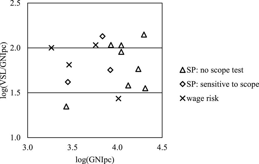
Figure 2 displays the ratios of estimated VSL to GNI per capita (in the same year as the VSL estimate) for the remaining 11 stated-preference surveys and four wage-risk studies. The scales are logarithmic (base 10). Overall, there is substantial variability in the ratio of VSL to GNI per capita, with most falling between roughly 40 (log ratio  $=$  1.6) and 107 (log ratio  $=$  2.0). The ratios appear similar for the four wage-risk studies (log ratios  $=$  1.4, 1.8, or 2.0) and the 11 stated-preference studies (log ratios  $=$  1.4 to 2.2), regardless of whether the latter test for sensitivity to scope. Of the studies in our review that fell within the plausible range of VSL to GNI per capita ratios (and hence are included in the figure), all that conducted a scope test found that WTP was sensitive to scope.

Figure 2 Ratio of VSL to GNI per capita (GNIpc).Footnote ²⁴

An alternative way to view the implications of these results is to estimate the income elasticity that would be needed to extrapolate from a VSL estimate for a high-income country to each of these VSL estimates. We rely on the U.S. Department of Health and Human Services (USDHHS) estimate in our comparisons because it is derived from a recent review and includes evaluation of both stated- and revealed-preference studies. We update the estimate to 2015 dollars, following the approach described in U.S. Department of Health and Human Services (2016).Footnote ²⁵ This yields a central VSL estimate of $9.4 million, or 162 times U.S. GNI per capita ($57,900) in that year. Relying instead on the USEPA or USDOT values, or on the values recommended in the Viscusi and Masterman studies, would lead to very similar results.

Again excluding implausibly high and low ratios, the income elasticity implied by comparing each of the remaining 15 ratios (reported in Appendix B) with the ratio for the USDHHS estimate ranges from 1.1 to 2.6 with a mean of 1.5 and a median of 1.4.Footnote ²⁶

These results seem reasonable, given that we expect that WTP for small changes in mortality risk will decline as income decreases. However, this comparison highlights the problems associated with using this literature as the basis for extrapolating VSL estimates across countries. First, as discussed in the previous sections, these studies were conducted in relatively few countries (primarily middle-income) and have several important limitations. Second, the mean income levels of the samples are not consistently reported, and may vary substantially from the estimates of GNI per capita (as well as GDP per capita) often used in cross-country transfers. Third, there is no clear relationship between VSL and income across these studies. Finally, regardless of whether the income measure used in these transfers is the sample mean reported by the authors or GNI or GDP per capita, the reliance on income to estimate inter-country variation ignores the cultural and other factors that may significantly influence these values.

It is difficult, if not impossible, to improve these estimates or validate these results without more high-quality research from low- and middle-income countries, which can be compared to the results of extrapolating from an estimate for a high-income country using alternative elasticities. More work is also needed to better understand how factors other than income affect these values.

It is unclear whether the uncertainty in the resulting VSL estimates is large relative to the uncertainty in other parameter values used in benefit-cost analysis. In some cases, the estimates of net benefits may be sensitive to these values; in others, whether a policy yields net benefits or which policy yields the greatest net benefits may not change regardless of which value is used.Footnote ²⁷

6.1 Population-average values

In the near term, to ease comparison with the findings of other benefit-cost analyses as well as examine related uncertainties, our recommendations for estimating the VSL in low- and middle-income countries include selecting a preferred estimate and conducting a standardized sensitivity analysis using common defaults.

The value featured as the preferred estimate should reflect the decision-making context, taking into account the characteristics of the individuals affected by the policy (such as income and age) and of the risk that the policy addresses (such as whether it results from illness or injury or is viewed as voluntarily incurred or under the individual’s control). Ideally, these values should be derived from a criteria-driven review of the WTP literature which identifies high-quality studies that are suitable for the context, including the characteristics of the risks and of the affected population. Meta-analysis and other methods are often helpful in synthesizing the results across studies.

The selection criteria and studies discussed in this paper provide a starting point for such a review. In addition to searching for more recent studies, analysts should review other sources for more information on best practices when developing criteria. For example, Johnston et al. (Reference Johnston2017) discuss best practices for stated-preference studies and Viscusi (Reference Viscusi2013) identifies the issues that may arise in conducting wage-risk studies. Neither source focuses specifically on estimating VSL in low- or middle-income countries; analysts will need to exercise judgment in applying the recommendations to the settings of concern.

Regardless of whether context-specific values are available, analysts should conduct a standardized sensitivity analysis to facilitate comparison to other studies and to explore the effects of uncertainties. The sensitivity analysis should follow the current practice of extrapolating a country-level population-average VSL estimate from the substantial research conducted in high-income countries, using data on GNI per capita (measured in international dollars using purchasing power parity) to estimate income, and an assumed income elasticity. The results should be reported in the local currency as well as in international dollars, to facilitate comparison to costs and to other policies that could be or have been implemented in that country.

The sensitivity analysis should use the following three estimates; option (a) is generally the preferred default, while options (b) and (c) are designed to align the results with the range applied in other research (see Table 2) and explore related uncertainties.

1. (a) VSL extrapolated from a U.S. estimate to the target country using an income elasticity of 1.5. The starting point for this calculation should be a U.S. VSL to GNI per capita ratio of 160, based on a U.S. VSL of $9.4 million and U.S. GNI per capita of $57,900. If this approach yields a value for the target country less than 20 times GNI per capita for that country, then 20 times GNI per capita should be used instead.

2. (b) VSL  $=$  160 * GNI per capita in the target country. This calculation applies the U.S. ratio to all countries, which is equivalent to using that ratio as the starting point and assuming income elasticity is 1.0.

3. (c) VSL  $=$  100 * GNI per capita in the target country. This calculation applies the OECD ratio to all countries, which is equivalent to using that ratio as the starting point and assuming income elasticity is 1.0.

Option (a) addresses concerns about the resources available for spending on mortality risk reductions in low- and middle-income countries. It seems reasonable to expect that the proportion of income devoted to attaining these small risk reductions will decrease as income decreases, rather than remain constant. More research on the values held by low- and middle-income populations is needed to estimate the rate of decrease with greater precision. In the interim, we recommend relying on the mean elasticity estimate (1.5) found when extrapolating from a U.S. value to the values found in our review in Section 4.3. While this extrapolation is subject to several limitations, an elasticity of 1.5 seems reasonable given the substantial income differences. The resulting VSLs should be limited to a lower bound of 20 times GNI per capita, to reflect the expectation that the population-average VSL will not be less than expected future income over the years of life remaining for the average adult.

Options (b) and (c) are designed to facilitate comparisons to studies that rely on approaches recommended in previous work as well as reflect uncertainties in the available research. The use of a constant VSL to GNI per capita ratio under both options is equivalent to assuming that income elasticity is 1.0 when extrapolating from a U.S. or OECD base value to a low- or middle-income country.

The first multiplier (160) is derived from the recommended U.S. values ($9.4 million VSL, $57,900 GNI per capita), rounded to two significant figures. It is similar to the ratio of the U.S. values used by other regulatory agencies and by Viscusi and Masterman in their exploration of publication-selection bias. Combining this base value with an elasticity of 1.0 likely provides a high-end estimate of the values for low- and middle-income countries.

The second multiplier (100) is derived from the OECD meta-analysis of stated-preference studies conducted globally. The studies that use this value as a starting point (OECD, 2016 and World Bank and IHME, 2016) rely on elasticities ranging from 0.8 to 1.2 depending on the study and the country; combining a base ratio of 100 with an elasticity of 1.0 essentially splits the difference. While the results are always lower than the values estimated under option (b), the relationship to the values estimating using option (a) depend on the income level of the target country.

We illustrate the results in Table 3, which summarizes the ratio of VSL to GNI per capita using these alternative approaches. In this example, we use six income levels that span the range of income levels found in low- and middle-income countries when expressed as GNI per capita based on purchasing power parity. As expected, for low-income countries, the estimates using an elasticity of 1.5 are much smaller than the estimates using the other approaches; for middle-income countries, the range is narrower. Estimates using each of these three approaches for all countries categorized as low- or middle-income (based on 2015 GNI per capita) are provided in a supplement posted on the journal’s website.

Table 3 Examples of extrapolated VSL estimates using alternative approaches.

Note: All results rounded to two significant digits.

It often requires several years for policy impacts to fully manifest. Analysts should also project the change in real income (measured as GNI per capita) in the country of concern that occurs over this time period and adjust the VSL estimates accordingly, using the approaches above. The underlying assumption is that income elasticities are the same over time as across different income groups at the same point in time.

These recommendations should be periodically revisited and revised to reflect the results of new research.

6.2 Adjustments for age and life expectancy

The approaches discussed above yield population-average estimates for an average-age adult. If the policy disproportionately affects the very young or the very old, analysts should also conduct sensitivity analyses using VSLY estimates. In such cases, analysts should derive a constant VSLY from each of the VSL estimates discussed above; i.e., the context-specific estimates (if any) and the three estimates that result from the standardized sensitivity analysis. Note that if the mean age of the individuals affected is the same as the mean age used in deriving VSLY from VSL, the results of applying each approach should be identical and this sensitivity analysis is not needed.

This constant VSLY should be calculated by first estimating the population-average VSL for the country affected by the policy, then dividing that VSL by undiscounted future life expectancy at the average age of the adult population in that country. In this calculation, “adults” would ideally be defined by the age range during which individuals are most likely to participate in the labor force, for consistency with the age ranges often included in the underlying VSL research. However, due to the difficulties inherent in defining this average age in some countries and the desire to promote consistency, analysts may wish to rely on the age that is equivalent to one-half of life expectancy at birth as a rough proxy. The constant VSLY that results should then be multiplied by the change in future life expectancy for those affected by the policy.

This calculation should not discount future years for two reasons. First, individuals may discount their own future years at a rate smaller than the rate at which they discount future consumption or other monetary values. Second, calculating VSLY using discounted future life years flattens the relationship between the value of reducing risk and age, making it more similar to the alternative of using the same VSL for all ages. For sensitivity analysis, it seems preferable to maintain the full effect of valuing life years equally rather than moderating the effect through the choice of some positive discount rate.

For example, if the population-average VSL for the country is $0.9 million and the life expectancy of an adult of average age in that country is 30 years, then the VSLY would be $30,000 based on simple division. Ideally, analysts would instead use a life table in this calculation, that indicates the likelihood of surviving each year of age conditional upon reaching that age. If the policy extends the life expectancy of individuals in the affected population by 10 years, the total value per individual affected would be $300,000 (10*$30,000).

If the analysis addresses deaths around the age of birth, the VSL and VSLY estimates described under the above recommendations can be used. However, analysts should also explore the impact of assigning positive values to mortality risk reductions that occur prior to birth.

6.3 Long-term recommendations

Over the longer term, more research is needed that explicitly addresses the value of mortality risk reductions in low- and middle-income countries. To support and encourage such studies, research methods tailored to this context should be further developed.

1. (1) Conduct additional research on WTP for mortality risk reductions in low- and middle-income countries: Substantial additional research is needed on the value of mortality risk reductions in these countries, given the importance of these estimates in policy analysis and the likely differences in preferences across members of different populations.

2. (2) Develop protocols for the conduct of these studies that are tailored to low- and middle-income settings. To encourage additional research and ease its implementation, more work is needed on developing approaches for data collection and analysis that can be feasibly implemented in low- and middle-income settings, which are designed to provide reasonably valid and reliable results. Such approaches should be tailored to the resources available for this type of research and should take into account the characteristics of these populations as well as the risks they face.

3. (3) Develop an easily accessible repository for valuation studies, that includes primary research as well as research that synthesizes the results. Many researchers in low- and middle-income countries may not have easy access to these studies, so will otherwise find it difficult to conduct the careful review that is needed to determine whether studies are applicable in particular settings and to form the foundation for new research.

Such additional research will help analysts, decision makers, and other stakeholders better understand the preferences of those affected, which can aid in policy implementation as well as evaluation. It also moves away from focusing largely on the effects of income differences, and encourages greater attention to other sources of variation such as differences in cultural norms and other context-specific factors.