


Introduction
As climate change intensifies, agricultural decision-makers are increasingly interested in the potential impacts such changes will make on crop productivity, and in the level of probability associated with the different impacts. Arguably, the most robust approach for simulating climate impacts on cropping productivity is the use of process-based models. These models account for complex interactions between the climate, soil, genotype and management affecting crop yield (Keating et al., Reference Keating, Carberry, Hammer, Probert, Robertson, Holzworth, Huth, Hargreaves, Meinke, Hochman, McLean, Verburg, Snow, Dimes, Silburn, Wang, Brown, Bristow, Asseng, Chapman, McCown, Freebairn and Smith2003; Stöckle et al., Reference Stöckle, Donatelli and Nelson2003; van Bussel et al., Reference van Bussel, Müller, van Keulen, Ewert and Leffelaar2011; Grassini et al., Reference Grassini, van Bussel, Van Wart, Wolf, Claessens, Yang, Boogaard, de Groot, van Ittersum and Cassman2015; Van Wart et al., Reference Van Wart, Grassini, Yang, Claessens, Jarvis and Cassman2015). However, meaningful crop model outputs (e.g. crop yield) can only be achieved when the parameters of the model have been appropriately calibrated, crop management options are realistically represented in the simulation, and the input weather data are accurate and reliable (Lamboni et al., Reference Lamboni, Makowski, Lehuger, Gabrielle and Monod2009; Liddicoat et al., Reference Liddicoat, Hayman, Alexander, Rowland, Maschmedt, Young, Hall, Herrmann and Sweeney2012; Grassini et al., Reference Grassini, van Bussel, Van Wart, Wolf, Claessens, Yang, Boogaard, de Groot, van Ittersum and Cassman2015). From this list of requirements, the lack of accurate and reliable weather data remains a common problem, particularly in developing countries.
Considerable effort has been devoted to developing protocols for enhancing observed weather data coverage for crop yield-gap analysis, crop yield projections and climate impact assessments (van Ittersum et al., Reference van Ittersum, Cassman, Grassini, Wolf, Tittonell and Hochman2013; van Wart et al., Reference van Wart, Grassini and Cassman2013; Watson and Challinor, Reference Watson and Challinor2013; Grassini et al., Reference Grassini, van Bussel, Van Wart, Wolf, Claessens, Yang, Boogaard, de Groot, van Ittersum and Cassman2015; Zhao et al., Reference Zhao, Siebert, Enders, Rezaei, Yan and Ewert2015). There is also an important number of global gridded data sets available, that have been produced using sophisticated methods and validated with a vast number of observations and data derived from remote sensing around the globe (Ruane et al., Reference Ruane, Goldberg and Chryssanthacopoulos2015; Hersbach et al., Reference Hersbach, Bell, Berrisford, Hirahara, Horányi, Muñoz-Sabater, Nicolas, Peubey, Radu, Schepers, Simmons, Soci, Abdalla, Abellan, Balsamo, Bechtold, Biavati, Bidlot, Bonavita, De Chiara, Dahlgren, Dee, Diamantakis, Dragani, Flemming, Forbes, Fuentes, Geer, Haimberger, Healy, Hogan, Hólm, Janisková, Keeley, Laloyaux, Lopez, Lupu, Radnoti, de Rosnay, Rozum, Vamborg, Villaume and Thépaut2020). However, these data sets cover a limited time period (between 20 and 40 years), and their validity relies on the density of weather stations, on the climate variables measured and record length of the available data, which is spatially highly variable and often low in the tropics, and in remote and rural areas. There is therefore the need to develop methods for reducing the dependency on a dense network of weather stations with high-quality and long-term observations, especially in data-sparse environments.
Regional land-use planning and on-farm management require a solid understanding of the long-term viability of production systems in a variable future climate. In fact, one of the core components of current agricultural decision-support systems is the risk profile – or cumulative probability – of crop yield under different management options (Hunt et al., Reference Hunt, van Rees, Hochman, Carberry, Holzworth, Dalgliesh, Brennan, Poulton, van Rees and Huth2006; Hochman et al., Reference Hochman, van Rees, Carberry, Hunt, McCown, Gartmann, Holzworth, van Rees, Dalgliesh, Long, Peake, Poulton and McClelland2009; Hayman et al., Reference Hayman, Wilhelm, Alexander and Nidumolu2010b; Hochman and Horan, Reference Hochman and Horan2018). The risk profile is particularly useful for reducing climate uncertainty and making better management decisions (Meinke et al., Reference Meinke, Stone and Hammer1996; Folland and Anderson, Reference Folland and Anderson2002; Domsch et al., Reference Domsch, Kaiser, Witzke, Zauer, Stafford, Werner, Stafford and Werner2003; Yao et al., Reference Yao, Xu, Lin, Yokozawa and Zhang2007; Hayman et al., Reference Hayman, Whitbread and Gobbett2008). Bracho-Mujica et al. (Reference Bracho-Mujica, Hayman and Ostendorf2019a) evaluated the dependency of the risk profile on climate record length and found that reliable risk profiles can be generated from short time periods of high-quality data. Furthermore, high-quality long-term rainfall and temperature records can be combined with high-quality temporal data from different locations to produce reliable risk profiles (Bracho-Mujica et al., Reference Bracho-Mujica, Hayman, Sadras and Ostendorf2019b). However, in all these studies the averaged climate data used for calculating the adjustment factors covered a long-term period (i.e. >100 years), which opens the question as to the extent to which this method can be used in common situations, where high-quality long-term data are spatially sparse and reliable long-term records to support interpolation or extrapolation are limited.
The goal of this study was to examine the applicability of a simple method of weather data adjustment for climate risk assessment, by testing the effects of short record lengths of averaged climate data on (i) the adjustment factors for precipitation, temperature, and global solar radiation and (ii) on the long-term risk profile of simulated wheat grain yield in the Australian grain belt.
Materials and methods
Study area
The current research focuses on wheat crops in the Australian grain belt. This is due to its importance to the Australian economy (Trewin, Reference Trewin2006; Australian Bureau of Statistics, 2020), its vulnerability to climate variability and change (Hammer et al., Reference Hammer, Holzworth and Stone1996; Potgieter et al., Reference Potgieter, Hammer and Butler2002) and the availability of one of the best weather data sets suitable for crop modelling (Jones et al., Reference Jones, Wang and Fawcett2009; Trewin, Reference Trewin2013). Previous studies on the assessment and improvement of the method of daily weather data adjustment for modelling risk profiles of simulated wheat yields have been conducted in the same area (Hayman et al., Reference Hayman, Wilhelm, Alexander and Nidumolu2010b; Liddicoat et al., Reference Liddicoat, Hayman, Alexander, Rowland, Maschmedt, Young, Hall, Herrmann and Sweeney2012; Bracho-Mujica et al., Reference Bracho-Mujica, Hayman and Ostendorf2019a, Reference Bracho-Mujica, Hayman, Sadras and Ostendorf2019b).
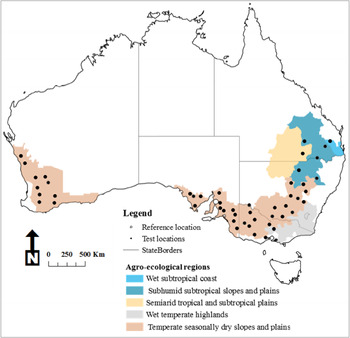
A total of 49 wheat-growing test sites within the grain belt were selected (Fig. 1 and Table 1), located in contrasting agro-ecological zones and with high-quality weather data. In addition, one spatial reference site was selected for the current study: Snowtown, in South Australia. The selection was made due to (a) its agricultural importance, (b) its position, located in the middle of the South Australian grain belt, (c) the high-quality long-term weather data required for crop yield simulations are available and (d) it allows for a comparison with previous studies.

Fig. 1. The Australian grain belt, reference location and test sites considered in this study. Data source: ABARES – BRS (2010).
Table 1. Location of the reference site (italic bold) and 49 test sites ordered clockwise, and agro-ecological zone, mean growing season precipitation (GSPrecip), seasonality, event-size index (τ), growing season maximum and minimum temperatures (GSMaxTemp and GSMinTemp), and global solar radiation (GSSolar)

Note: Period 1901–2000.
a Agro-ecological zones as defined in (Williams et al., Reference Williams, Hook and Hamblin2002).
b Seasonality (Walsh and Lawler, Reference Walsh and Lawler1981).
c τ (Sadras, Reference Sadras2003).
Daily precipitation, maximum and minimum temperatures and solar radiation data from these sites were obtained from the SILO patch point database (Scientific Information for Land Owners) (Jeffrey et al., Reference Jeffrey, Carter, Moodie and Beswick2001). The period used was 1901–2000, avoiding the bias of the extreme Millennium drought (van Dijk et al., Reference van Dijk, Beck, Crosbie, de Jeu, Liu, Podger, Timbal and Viney2013; Verdon-Kidd et al., Reference Verdon-Kidd, Kiem and Moran2014), which alters the shape of the risk profile.
Adjustment of daily weather data
Risk profiles were derived from the simulated wheat grain yield in two ways: using actual weather data from each study site, and using adjusted weather data from the reference location. ‘Adjusted weather data’ refers to daily weather series (for precipitation, maximum and minimum temperatures and global solar radiation) recorded at the reference location (Snowtown) and later systematically perturbed using adjustment factors (or delta factors). Adjustment factors are variable and site-specific and represent the difference between the reference and a given test site.
To account for the intra-annual variability of the climate variables, adjustment factors were calculated at the seasonal and monthly levels. For the calculation of seasonal adjustment factors, daily climate data – for all climate variables – were averaged from April to October (growing season). Monthly adjustment factors were only calculated for the maximum and minimum temperatures, by averaging daily data for each month within the growing season. The record length used for calculating those averages varied. For the reference site, the full period of weather records was used (i.e. 100 years from 1901 to 2000). For each test site, the record length was 10, 20, …, 100 years in 10-year steps – in order to account for the effect of short climate series on the estimation of adjustment factors and the long-term risk profiles. Adjustment factors calculated with the full record were referred to as the ‘100-year adjustment factor’. Adjustment factors are listed in Supplementary Tables S1–S5.
Once the average climate data were calculated for the different record lengths and aggregation levels, daily weather data for the reference location were perturbed using adjustment factors summarized in Table 2. The precipitation series were first adjusted with a single factor ${\rm Preci}{\rm p}_{{\rm s}_{{\rm AF}}}$ , which represents the difference in average growing-season precipitation between the test site and the reference location, expressed as a percentage. The adjustment factor for global solar radiation (${\rm Sola}{\rm r}_{{\rm s}_{{\rm AF}}}$
 ) was calculated similarly. In the case of maximum and minimum temperatures, two adjustment factors were calculated. Firstly, a seasonal factor (${\rm Tem}{\rm p}_{{\rm s}_{{\rm AF}}}$
 ), calculated as the difference in average growing-season temperature between a given test site and the reference location, is expressed in °C. Secondly, a monthly factor (${\rm Tem}{\rm p}_{{\rm m}_{{\rm AF}}}$
 ), calculated as the monthly difference in temperature between the reference and a given test site. Weather data were then adjusted by multiplying (precipitation and global solar radiation) or adding (temperature) the corresponding factor of every daily record (Table 2).
Table 2. Equations for calculating adjustment factors of weather data

Note: GSPrecip, GSMaxTemp, GSMinTemp, and GSSolar refer to the long-term average growing season precipitation, maximum temperature, minimum temperature, and global solar radiation, respectively. MaxTempm and MinTempm refer to the long-term monthly temperature averages for months m = 4, 5, …, 10, within the growing season. The terms ref and k refer to the reference location and test sites.
Adjustment factors calculated with a variable record length (<100 years) were compared with the 100-year adjustment factor. This comparison was established at a test site level using the difference of any given adjustment factor and climate variable from the 100-year adjustment factor.
Step-wise addition of weather data adjustments
Five types of adjustments were applied, resulting from the combination of variables included and level of aggregation (Table 3). For example, the Precips consisted of adjusting the daily weather data for precipitation, using a seasonal aggregation, whereas temperatures and solar radiation were unadjusted. PrecipsTempmSolars, was the most complete adjustment, in which all the climate variables from the reference site were adjusted using two different aggregations for the calculation of the average climate data (i.e. seasonal for precipitation and solar radiation, and monthly for temperature).
Table 3. Step-wise adjustment applied to the daily weather data at the reference location

Note: Weather data at the reference site is adjusted by a seasonal adjustment factor for precipitation only (Precips), seasonal adjustment factors for precipitation and temperatures only (PrecipsTemps), a seasonal adjustment factor for precipitation and monthly adjustment factors for temperatures (PrecipsTemps), a seasonal adjustment factor for precipitation, temperatures and global solar radiation (PrecipsTempsSolars), and, a seasonal adjustment factor for precipitation and global solar radiation, and monthly adjustment factors for temperatures (PrecipsTempmSolars)
Crop yield simulations
Wheat grain yield was simulated with APSIM (Agricultural Production Systems Simulator Model) Version 7.8 (Keating et al., Reference Keating, Carberry, Hammer, Probert, Robertson, Holzworth, Huth, Hargreaves, Meinke, Hochman, McLean, Verburg, Snow, Dimes, Silburn, Wang, Brown, Bristow, Asseng, Chapman, McCown, Freebairn and Smith2003; Holzworth et al., Reference Holzworth, Huth, DeVoil, Zurcher, Herrmann, McLean, Chenu, van Oosterom, Snow, Murphy, Moore, Brown, Whish, Verrall, Fainges, Bell, Peake, Poulton, Hochman, Thorburn, Gaydon, Dalgliesh, Rodriguez, Cox, Chapman, Doherty, Teixeira, Sharp, Cichota, Vogeler, Li, Wang, Hammer, Robertson, Dimes, Whitbread, Hunt, van Rees, McClelland, Carberry, Hargreaves, MacLeod, McDonald, Harsdorf, Wedgwood and Keating2014). APSIM has been locally calibrated, widely tested and extensively used for climate risk in the study area (Asseng et al., Reference Asseng, Bar-Tal, Bowden, Keating, Van Herwaarden, Palta, Huth and Probert2002, Reference Asseng, Zhu, Wang, Zhang, Sadras and Calderini2015; Luo et al., Reference Luo, Bellotti, Williams and Bryan2005, Reference Luo, Bellotti, Williams and Wang2009; Robertson et al., Reference Robertson, Rebetzke and Norton2015).
Observed and adjusted daily weather data calculated for variable periods were used as model inputs. To capture the effects of climate and alternative weather inputs in the current study, the soil type and management practices were kept constant, and assumed no limitation by nitrogen, pests or diseases. To exclude the interaction between the sowing time and climate (Luo et al., Reference Luo, Bellotti, Williams and Wang2009; Hayman et al., Reference Hayman, Whitbread and Gobbett2010a), one fixed sowing date was simulated (14 May); sowing density was set to 180 plants/m2, with a 30 mm sowing depth and 250 mm row spacing. Crop parameters used were those from locally adapted varieties, Mace (an early maturing variety) for the winter-rainfall regions of Western Australia, South Australia, Victoria and southern New South Wales; and Gregory (a medium maturing variety) for the summer-rainfall locations of northern New South Wales and Queensland. Crop parameters are summarized in Table 4.
Table 4. Cultivar-specific parameters for wheat cultivars Mace and Gregory used for the parameterisation of APSIM

The soil used has a sandy texture, organic carbon content of 0.7% (0–10 cm), rooting depth of 100 cm and 80 mm of plant available water content (PAWC). Key soil characteristics are presented in Table 5. Initial water and nitrogen contents were reset every year on the 1st of April to exclude the effects of previous seasons, as suggested in the literature (Sadras and Rodriguez, Reference Sadras and Rodriguez2010; Luo et al., Reference Luo, Wen, McGregor and Timbal2013). The initial soil water content was set to full profile, filled from the top layer to ensure crop establishment (Bell et al., Reference Bell, Lilley, Hunt and Kirkegaard2015), and the initial nitrogen level was set to 100 kg N/ha as urea at sowing.
Table 5. Key soil characteristics used for the initialisation of APSIM
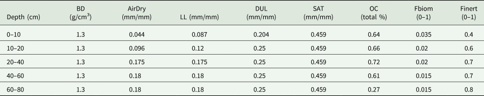
Note: BD, bulk density; AirDry, Air-dry soil water content; LL, Lower limit of plant available water or permanent wilting point; DUL, drained upper limit of plant available water or field capacity; SAT, saturated soil water content; OC, Organic carbon; Fbiom, fraction of susceptible organic carbon; Finert, fraction of organic carbon that is not susceptible to decomposition.
Risk profiles of modelled wheat grain yields (MWGYs)
Risk profiles were defined as the cumulative probability curve of the annual MWGY for each site, type of weather adjustment (Table 3), and record length. Yields were ranked and corresponding percentiles were calculated. Risk profiles of the MWGYs across the types of adjustments and record lengths were compared using Q:Q plots. Statistics for the comparisons included the root mean squared error (RMSE, Eqn (1)), and the bias (Eqn (2)), overall percentile classes p at each of the 49 test sites j as follows:

and

The bias of the MWGY represents the difference between the risk profiles of MWGY built with weather data adjusted with long-term adjustment factors and those built with data adjusted with shorter record lengths, as illustrated in Fig. 2.

Fig. 2. Comparison of two risk profiles of MWGY, using recorded weather data at the study site Nyngan (NSW, Australia), and using adjusted weather data from a reference site with a 10-year adjustment factor. Bias (normalized) at percentile 50th corresponds to the difference between both MWGY normalized with the mean of the MWGY modelled with observed weather data at the study site.
Both indices, RMSE and bias, were mapped for every type of adjustment applied to the reference location, to (i) visualize the spatial variation of the performance indices, (ii) compare the regions and (iii) determine the effect of adjusting a particular set of climate variables on the robustness of the MWGY risk profiles. Construction and statistical analysis of the risk profiles of the MWGY were performed using R software (R Development Core Team, 2020) and maps were created using ArcGIS® software (ESRI 2015).
Results
Long-term adjustment factors and weather data record lengths
The calculation of 100-year adjustment factors is based on the difference in the long-term growing-season average of the reference and test sites. Here, we examined the sensitivity of four adjustment factors – for precipitation, maximum temperature, minimum temperature and solar radiation – to the length of the weather record (Figs 3 and 4).

Fig. 3. Departures from the 100-year adjustment factors relative to those calculated with shorter record lengths in 49 locations of the Australian wheat-belt. From left to right weather records of the reference location were adjusted as a function of seasonal precipitation (PrecipsAF), seasonal maximum temperature (MaxTempsAF), seasonal minimum temperature (MinTempsAF) and seasonal solar radiation (SolarsAF). IQR refers to the inter-quartile range.

Fig. 4. Departures from the 100-year monthly adjustment factors for maximum and minimum temperatures relative to those calculated with shorter record lengths in 49 locations of the Australian wheat-belt. Weather records of the reference location were adjusted as a function of the monthly maximum temperature (MaxTempmAF), and the seasonal minimum temperature (MinTempmAF). IQR refers to the inter-quartile range.
All seasonal adjustment factors were sensitive to the record length, especially for records shorter than 30 years. In the case of precipitation, departures ranged from −14 and 20% for the 10-year series and dropped within the range −10 and 10% with 40 or more years (Fig. 3). Long-term adjustment factors for temperatures were mostly underestimated with shorter records; series of 10 years diverged by −0.9 and 0.3°C for maximum and between −1.2 and 0.5°C for minimum temperature in relation to 100-year series. At most test sites, these departures were reduced to −0.5 to 0.5°C with records longer than 30 years. Solar radiation was the variable with the lowest sensitivity to the record length, with departures ranging between −2.4 and 3%, and with a slight increment at record lengths between 30 and 60 years of weather data.
The effect of record length on the calculation of adjustment factors for maximum and minimum temperatures was stronger at the monthly level (Fig. 4). Particularly, record lengths equal and shorter than 40 years produced the highest departures of adjustment factors from the 100-year factors, independent of the month. However, the departures were higher during the transition months, i.e. April and May for the minimum temperature factors, and April and October for the maximum temperature factors. At most test sites, departures were within −0.5 to 0.5°C with records longer than 40 years (Fig. 4).
Long-term risk profiles of MWGY and weather data record lengths
The use of averaged climate data for record lengths shorter than the 100-year period affected the long-term risk profile of MWGY. In Fig. 5, all the test sites are included, but we only present three of the five types of adjustments used in this study (i.e. Precips, PrecipsTempm and PrecipsTempmSolars). The adjustments PrecipsTemps and PrecipsTempsSolars are not shown since lower bias was obtained with the PrecipsTempm and PrecipsTempmSolars adjustments (bias and RMSE values are summarized in the Supplementary Material, Table S6).

Fig. 5. Bias (%) of the risk profiles of MWGYs built with adjustment factors calculated with variable record lengths of weather data across the different types of adjustments incorporated. Bias compares the risk profiles obtained with weather data observed at the study site for the period 1901–2000, and those obtained with scaled weather data using a variable record length of size n (n = 10, 20, …, 100) for calculating the seasonal adjustment factors for precipitation, maximum and minimum temperatures and solar radiation. The pie charts show the proportion of test sites within different categories of bias.
The bias of MWGY risk profiles varied spatially (Fig. 5, Table S6). Test sites in the temperate agro-ecological zones with winter-dominant rainfall (Fig. 1) had the lowest biases across all types of adjustments and climate data record lengths (Fig. 5). Long-term risk profiles of MWGY of test sites in wet subtropical coast, subhumid subtropical, and semiarid tropical and subtropical locations were mostly overestimated, with the greatest biases in the study area (Fig. 5). The low matching observed in northern and north-eastern sites is exacerbated by the shortest climate data record lengths. Matching in the −10 to 10% range was only achieved in those sites with record lengths of 80 or more years and including all adjustments.
The proportion of test sites in which the long-term risk profiles were estimated within −5 to 5% bias improved with extra adjustments (precipitation, temperature, and solar radiation) and as the record length was increased (Fig. 5, pie charts). Using the shortest record length (10 years) the simplest adjustment (Precips) produced matching of long-term risk profiles in range −10 to 10% for 41% of the sites, which increased to 49% with the PrecipsTemps adjustment, 53% with the PrecipsTempm, and up to 60% of the sites with the most complete types of adjustments (PrecipsTempmSolars). These proportions did not change substantially for record lengths between 10 and 50 years of averaged climate data. However, using averaged climate data for a period of 60 or more years increased the number of sites with bias within −10 and 10%. For example, with the Precips adjustment, the number of sites went from 47% (60 years of record length) to 51% (with 100 years of record length), while the use of the PrecipsTempmSolars adjustment the number of sites increased from 59 to 86% of the test sites.
Discussion
The effect of limited temporal coverage of averaged climate data on the validity of a method for scaling weather data for extrapolation of long-term risk profiles for simulated crop yields was examined in the current study. This method uses averaged climate data for precipitation, temperature and solar radiation to scale daily weather data from a reference site with long-term records. Scaled daily data are then used for simulating crop yields and building long-term risk profiles, demonstrating that the method tested is able to provide a robust spatial extrapolation of risk profiles, even if the temporal extent of the averaged climate data is limited.
The adjustment factors showed different responses to the record length used for averaging the climate data. As expected, sensitivity to record length ranked precipitation > minimum temperature > maximum temperature > global solar radiation. This response is primarily driven by the natural variability of these climate variables, which is considerably higher for precipitation, and lower for temperature and solar radiation (Jäger, Reference Jäger, Parry, Carter and Konijn1988; Von Storch and Zwiers, Reference von Storch and Zwiers1999). Despite this fact, reasonable estimates of the long-term adjustment factors were obtained when using averaged data for shorter time periods. In the case of precipitation, at least 40 years were necessary to obtain departures of the long-term adjustment factor within the range −10 and 10% (Fig. 3). For both, the maximum and the minimum temperatures, a minimum of 30 years at most test sites produced departures spanning from −0.5 to 0.5°C at seasonal level (Fig. 3), and a minimum of 40 years for monthly adjustment factors (Fig. 4). For solar radiation, 10 years records produced departures between −2.4 and 3% (Fig. 3). This finding is relevant for potential future applications of the method in data-sparse environments.
The long-term risk profile of MWGY was also sensitive to the temporal coverage of the averaged climate data (Figs 3–5). However, the number of adjustments applied had a major effect on the long-term risk profile. The most complete adjustment (PrecipsTempmSolars) produced acceptable matching of risk profiles in ~60% of the test sites using record lengths between 10 and 50 years. This proportion of sites was higher than the 51% of sites when 100 years of record length was used with only precipitation adjusted. There was also a spatial pattern in the matching of risk profiles. Better results were obtained in winter-rainfall sites, which required fewer adjustments and record lengths, while most summer-rainfall sites required more adjustments and the longest period of averaged climate data. This could be explained by the similarity in climates in the reference location and the western, southern and south-eastern sites, all falling in temperate regions (Williams et al., Reference Williams, Hook and Hamblin2002) with comparable rainfall patterns in terms of amount, seasonality and size of events (Table 1; Williamson, Reference Williamson2007).
The current study uses a simple method for extrapolating risk profiles described in Hayman et al. (Reference Hayman, Wilhelm, Alexander and Nidumolu2010b) and Liddicoat et al. (Reference Liddicoat, Hayman, Alexander, Rowland, Maschmedt, Young, Hall, Herrmann and Sweeney2012) and further developed in Bracho-Mujica et al. (Reference Bracho-Mujica, Hayman, Sadras and Ostendorf2019b), and expand in several aspects. Firstly, the extrapolation method was tested under a non-uncommon situation of having limited daily weather data (in terms of both temporal and spatial coverage) for estimating modelled risk profiles. Secondly, it endorses the incorporation of the monthly adjustment of maximum and minimum temperatures accounting for the role of temperature on crop development (Bracho-Mujica et al., Reference Bracho-Mujica, Hayman, Sadras and Ostendorf2019b). Thirdly, it demonstrates the importance of the number of adjustments over the record length of the averaged climate data, which was not tested in previous studies. Fourthly, results from this study allow us to estimate the minimum record length necessary for calculating robust adjustment factors. This enables to produce more robust matching between MWGY risk profiles and illuminate similarities and differences among and across locations on a continental scale.
Crop modellers working in data-sparse environments can use these results to save computational time on climate data, which frees up resources for other factors such as soil types. Farmers and agronomists can use the findings to judge the reliability of simple climate adjustments for risk analysis based on modelled yield. The extensive comparison across the Australian grain belt not only highlights the importance of adjusting the most critical climate variable determining wheat yield, precipitation, but also points to the need to adjust temperature and solar radiation to improve the estimation of the risk profiles of modelled crop yields.
The impact of the temporal coverage of the averaged climate data was explored in the current research, assuming that all climate variables had the same record length. However, another interesting aspect to explore in future studies would be the impact of different temporal coverages across all the climate variables. Nevertheless, these findings provide evidence that temporal coverage is not as important as the type and number of adjustments used for the determination of robust risk profiles of MWGY.
The use of the method for scaling climate data has been rigorously tested across multiple sites and climates within the Australian grain belt, and results demonstrate the power of this simple method for extrapolating the long-term risk profiles of MWGY. However, it is important to note that this method was not intended for estimating year-to-year crop yields but for long-term risk profiles of crop yields. Furthermore, it is important to highlight that the approach used in the current study did not account for the spatial variability of soils and management practices (i.e. sowing dates and nitrogen fertilization), which allowed examination of the maximum impact of climate on the method of extrapolation of risk profiles.
Conclusions
A simple method for adjusting daily weather data for extrapolating risk profiles was tested across the entire Australian-grain belt. Risk profiles based on process-based models could be accurately extrapolated even if only short climate data series were available to compute adjustment factors. The results indicated that although the temporal coverage of the climate data used for adjusting daily records is important, the adjustment of all climate variables (i.e. precipitation, temperatures and solar radiation) produced the most reliable estimations of modelled yield risk across a large area, encompassing a diversity of climates.
Supplementary material
The supplementary material for this article can be found at https://doi.org/10.1017/S0021859621000253
Acknowledgements
We thank Alison-Jane Hunter for the proofreading of this paper.
Financial support
This research was supported by an Australia Awards Scholarship (AAS), from the Australian Department of Foreign Affairs and Trade to G. Bracho-Mujica. P.T. Hayman time supported by Australian Government Rural R&D for Profit.
Conflict of interest
The authors declare there are no conflicts of interest.
Ethical standards
Not applicable.


 Open access