


INTRODUCTION
Simultaneous equation statistical models are an attractive method for analysing interactions among components of animal systems directly. An application of these models is in bio-energetics of animal growth, because it is preferable to analyse protein deposition (PD) and lipid deposition (LD) data using simultaneous equations statistical models (Koong Reference Koong1977; van Milgen & Noblet Reference van Milgen and Noblet1999; Strathe et al. Reference Strathe, Danfær, Chwalibog, Sørensen and Kebreab2010a ). However, they require utilization of additional parameters, which is computationally costly and hence these models have been applied mainly to larger datasets. For instance, Strathe et al. (Reference Strathe, Danfær, Chwalibog, Sørensen and Kebreab2010a ) analysed 384 energy balances, which can be considered a large dataset for metabolic studies. These studies require expensive equipment and labour, so they often produce sparse datasets. As a consequence, parameter identifiability becomes an issue, which leads to poor convergence of the non-linear estimation routine, i.e. parameter estimates with large standard errors (s.e.) and point estimates of key parameters that may be scientifically unreasonable.
In Bayesian paradigm, prior information can be synthesized through formal statements of probability because model parameters are viewed as random variables with associated probability distributions, so-called ‘priors’ to the parameters (Gelman et al. Reference Gelman, Carlin, Stern and Rubin2004). The inclusion of previous knowledge is a fundamental and integral part of the modelling process – for example, parameters describing partial efficiencies of utilizing metabolizable energy (ME) above maintenance (MEM) for protein deposition (PD; k p ) and LD (k f ) and the exponent scaling the metabolic body size (b), are known a priori because the bioenergetics of growth have been studied for decades. The prior distributions are subsequently updated with regard to the data at hand. The resulting, so-called ‘posterior probability distributions’, or ‘posteriors’ for short, are consistent with both the experimental data and the priors, as the posteriors are derived from the product of the likelihood of the data and the prior probability of the parameters. A Bayesian approach has recently been described for the analysis of energy balance data in dairy cows as a robust framework for integration and extraction of information (Strathe et al. Reference Strathe, Dijkstra, France, Lopez, Yan and Kebreab2011).
The objective of the current study was to develop Bayesian simultaneous equation models for modelling energy intake and partitioning in growing pigs.
MATERIALS AND METHODS
All experimental procedures complied with the Danish Ministry of Justice, Law No. 382 (10 June 1987) and Act No. 726 (9 September 1993), regarding animal experimentation and care.
Experimental procedure
The pigs used in the study were crosses of Yorkshire × Landrace sows and Duroc boars. Eighteen pigs of three genders (barrow (male pig castrated before puberty), boar and gilt), originating from six litters were used and hence there were six pigs per gender. The pigs were obtained from the swine herd at Foulum Research Centre (Denmark). The first 12 pigs were subjected to three balance periods, whereas the last six pigs were subjected to four periods, covering the growth phase from 20 to 150 kg body weight (BW). During the growth phase, the pigs were fed four diets (described later in this section) in the corresponding intervals: 25–45, 45–65, 65–100 and 100–150 kg BW. The balance periods were planned to be done in the middle or last part of each interval. All balance periods lasted 7 days in metabolism cages, with days 4 and 5 in the respiration chambers. One barrow was omitted from the dataset due to illness in the first balance period. A total of 56 energy balances including 16 for barrows, 20 for boars and 20 for gilts were measured. During the collection and balance periods, the pigs were kept in stainless steel metabolism cages in the respiration chambers. Feed allowance approximated ad libitum feed intake. Faeces and urine were collected quantitatively during the 7-day collection period. Gas exchange and heat production (HP) were measured for 48 h on days 3 and 4. BW over each balance period was calculated as the mean of initial and final BW during the period. The calculation of ME included energy losses in faeces, urine, methane and hydrogen. The average daily HP was calculated according to Brouwer (Reference Brouwer and Blaxter1965). Total energy gain over the balance period was obtained as the difference between ME intake (MEI) and HP; its partition between protein and lipid gain was calculated by assuming that protein gain (6·25 × nitrogen (N) retention) contained 23·8 kJ/g (ARC 1981). Nitrogen retention was calculated as the difference between N intake and N losses in faeces and urine. The experimental procedure of conducting respiration and energy balance trials at Foulum Research Centre is described in full by Jorgensen et al. (Reference Jorgensen, Zhao and Eggum1996).
The diets were based on barley, wheat and soybean meal, and were formulated to meet nutrient requirements according to Danish nutritional standards. Their ingredient and chemical compositions are presented in Table 1. The pigs were individually housed under thermoneutral conditions and given ad libitum access to feed and water when they were not subjected to determination of nutrient and energy balance.
Table 1. Nutrient and energy composition of experimental diets

* Estimated according to Just (Reference Just1982), Just et al. (Reference Just, Jørgensen and Fernández1983) and Boisen & Fernandez (Reference Boisen and Fernandez1997).
† Non-starch polysaccharides + lignin.
Statistical model
It was assumed that multiple observations from the pig were independent because diets were changed during the consecutive balance periods. Also, a preliminary analysis showed that variance components associated with structural model parameters were poorly estimated, because it was difficult to estimate pig specific MEI, PD and LD curves with only three observations per pig and only 17 pigs. The distribution of the data conditional on model parameters is
 $$y_{ijk} |{\bf \beta} _i, k_p, k_f, b,{\bf \Sigma} \sim {\rm MVN}(\,f\,({\bf \beta} _i, k_p, k_f, b,{\rm BW}_{ij} )_k, {\bf \Sigma} )$$
where y ijk denotes the kth observed response (MEI, PD and LD, all expressed in MJ/day) related to the ith gender (barrow, boar and gilt) at the jth BW (1, 2, …, n i ); f(β i , kp, kf, b, BW ij ) k denotes the expected MEI, PD and LD values given by the simultaneous equations, which are described in detail below. The vector of structural parameters is specific to the ith gender and denoted by β i . The elements in β i are also specific to the equation format, equating the expected values, and its attributes and dimensions are presented below. Parameters k p , kf and b are the partial efficiencies and metabolic exponent parameter, respectively, which are dimensionless quantities. The variance–covariance matrix Σ describes the residual variability in the three responses. The introduction of a multivariate normal (MVN) distribution assumes that the responses are correlated (Strathe et al. Reference Strathe, Danfær, Chwalibog, Sørensen and Kebreab2010a ). Moreover, measurement errors that might have occurred in the determination of ME, PD or LD are assumed to be correlated. This is an important model feature in the calculation of energy balances and their interrelationships, and it represents an extension of the previous framework proposed by Strathe et al. (Reference Strathe, Danfær, Chwalibog, Sørensen and Kebreab2010a ).
Simultaneous equations describing energy partitioning
MEI (MJ/d) is described by an exponential function, which is used frequently to model intake in growing pigs (e.g. ARC 1981). The function has two parameters that can be interpreted as the asymptotic (maximum) MEI M (MJ/day) and the fractional change in MEI due to a change in BW, k (1/kg), respectively. The energy partitioning is modelled as follows: ME available for growth (MEG, MJ/day) is calculated as the difference between MEI and ME for maintenance (MEM, MJ/day). The fraction (F, dimensionless) of MEG available for PD is assumed not to be constant, but a linear function of BW. Multiplication of MEG by F and by 1−F gives ME for PD (MEPD, MJ/day) and ME for LD (MELD, MJ/day), which are used with efficiencies k p and k f , respectively. Combination of these equations proposed by van Milgen & Noblet (Reference van Milgen and Noblet1999) with the equation for predicting MEI results in the following simultaneous equations:
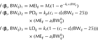 $$\eqalign{\,f\,({\bf \beta} _i, {\rm BW}_{ij} )_1 = & \; {\rm MEI}_{ij} = M_i (1 - {\rm e}^{ - k_i \times BW_{ij}} ) \cr f\,({\bf \beta} _i, {\rm BW}_{ij} )_2 = & \; {\rm PD}_{ij} = k_p (c_i - d_i ({\rm BW}_{ij} - 25)) \cr & \times ({\rm ME}_{ij} - a_i {\rm BW}_{ij}^b ) \cr f\,({\bf \beta} _i, {\rm BW}_{ij} )_3 = & \; {\rm LD}_{ij} = k_f (1 - (c_i - d_i ({\rm BW}_{ij} - 25))) \cr & \times ({\rm ME}_{ij} - a_i {\rm BW}_{ij}^b )} $$
Maintenance is specified as ME M =a i BW b where a i is the gender-specific maintenance requirement (MJ ME/(kg BW b × day)) and b is the metabolic exponent (dimensionless). It is assumed that F decreases linearly with BW, i.e. F ij =c i −d i (BW ij − 25). Here c i is the fraction of MEG used for PD at 25 kg BW and d i (1/kg) is the change in F per kg BW change. The gender-specific parameter vector is β i = [M i , ki, ai, ci, di ] T .
Another set of MEI, PD and LD equations, which provides additional insight into the partitioning of ME during growth, is presented below. This approach requires a functional specification of the PD curve. The concept of an upper limit for PD in growing pigs is widely accepted, as pigs are limited by either their genetic or feed intake capacity (at earlier stages of growth). The Gompertz function is often the preferred function for representing the pattern of maximum PD (PDmax) in pigs (Whittemore & Green Reference Whittemore and Green2002) and it can be parameterized to express the BW at maximum rate of PD (BWPDmax, kg) and the associated PDmax (MJ/day) (Strathe et al. Reference Strathe, Danfær, Chwalibog, Sørensen and Kebreab2010a ), when PD is expressed as a function of BW. Strathe et al. (Reference Strathe, Danfær, Chwalibog, Sørensen and Kebreab2010a ) used the specialized Gompertz function in combination with the Michaelis–Menten function to model effects of ME supply on growth. However, the pigs used in the present study were all fed close to ad libitum and thus the effect of energy supply on PD cannot be separated from the stage of growth. The equation set is given as
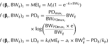 $$\eqalign{\,f\,({\bf \beta} _i, {\rm BW}_{ij} )_1 = & \; {\rm MEI}_{ij} = M_i (1 - {\rm e}^{ - k \times {\rm BW}_{ij}} ) \cr f\,({\bf \beta} _i, {\rm BW}_{ij} )_2 = & \; {\rm PD}_{ij} = \displaystyle{{{\rm PD}_{{\rm max}_i}} \over {{\rm BW}_{{\rm PDmax}_i}}} {\rm BW}_{ij} \cr & \times {\rm log}\left( {\displaystyle{{{\rm BW}_{{\rm PDmax}_i} \times {\rm e}} \over {{\rm BW}_{ij}}}} \right) \cr f\,({\bf \beta} _i, {\rm BW}_{ij} )_3 = & \; {\rm LD}_{ij} = k_{\rm f} ({\rm ME}_{ij} - a_i \times {\rm BW}_{ij}^b - {\rm PD}_{ij} /k_{\rm p} )} $$
The gender-specific parameter vector is β
i
=
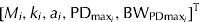 $ [M_i, k_i, a_i, {\rm PD}_{{\rm max}_i}, {\rm BW}_{{\rm PDmax}_i} ]^{\rm T} $
and e is the exponential to 1. Equation sets (2) and (3) require the same number of parameters to be estimated, but equation set (3) provides complementary information about energy utilization in growing pigs, i.e. PDmax estimation. The fraction of MEG partitioned for PD can be calculated from equation set (3) as
$ [M_i, k_i, a_i, {\rm PD}_{{\rm max}_i}, {\rm BW}_{{\rm PDmax}_i} ]^{\rm T} $
and e is the exponential to 1. Equation sets (2) and (3) require the same number of parameters to be estimated, but equation set (3) provides complementary information about energy utilization in growing pigs, i.e. PDmax estimation. The fraction of MEG partitioned for PD can be calculated from equation set (3) as
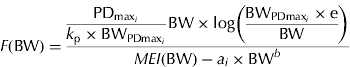 $$F({\rm BW}) = \displaystyle{{\displaystyle{{{\rm PD}_{{\rm max}_i}} \over {k_{\rm p} \times {\rm BW}_{{\rm PDmax}_i}}} {\rm BW} \times {\rm log}\left( {\displaystyle{{{\rm BW}_{{\rm PDmax}_i} \times {\rm e}} \over {{\rm BW}}}} \right)} \over {MEI ({\rm BW}) - a_i \times {\rm BW}^b}} $$
Clearly, F changes non-linearly during the course of growth. The quantity F is suggested here as a measure of the priority for PD in energy terms. To facilitate interpretation (when needed), the results are reported in grams per day by assuming 23·8 kJ/g of protein and 39·6 kJ/g of lipid (ARC 1981).
Specification of priors
The prior specification is concerned with assigning probability distributions to β i , Σ, k p , kf and b. Priors for β i and Σ are
 $${\bf \beta} _i \sim {\rm MVN}({\bf \mu, H});{\rm} {\bf \Sigma} \sim {\rm IW}({\bf R},\rho )$$
where IW(·,·) denotes the inverse-Wishart distribution. At this point, numerical values for μ, H, R and ρ must be stated. Here, μ = [0,…, 0]T and H = 1002×I are used, where I is the identity matrix. The prior for β i is minimally informative, leading to no restriction on the partitioning of ME between growth and maintenance. The inverse-Wishart distribution was selected to represent the prior for the residual variance–covariance because it is the only closed form distribution that naturally imposes the appropriate constraint, i.e. positive definiteness. Hence, R=I and ρ = 3, which specifies the vaguest possible proper prior for Σ.
The above equation systems cannot be solved properly without utilization of numerical information about some of the parameters. Table 2 represents a compilation of values from the literature for the partial efficiencies k p and k f , which suggest that the efficiencies of PD and LD are c. 0·6 and 0·8, respectively. Hence, conservative prior distributions can be deduced from Table 2. Normal and uniform distributions are specified by assuming that k p ∼N(0·60, 0·102) or k p ∼U(0·40, 0·80) and k f ∼N(0·80, 0·102) or k f ∼U(0·60, 1·00). The 0·95 confidence intervals (CIs) for parameters k p and k f specified by the normal distributions are (0·40–0·80) and (0·60–1·00), respectively. However, the biological interpretation of the assigned prior distributions is different because the normal distribution states that it is more likely that k p is 0·6 than 0·4, whereas the uniform distribution states that these values are equally likely. Likewise, the prior for b is b∼N(0·60, 0·102) or b∼U(0·40, 0·80). Finally, the two different prior distributions also constitute a sensitivity analysis because two sets of posterior distributions are produced, and hence the conclusions may or may not differ between the choices of priors (Gelman et al. Reference Gelman, Carlin, Stern and Rubin2004).
Table 2. Compilation of literature values for the partial efficiencies k p and k f
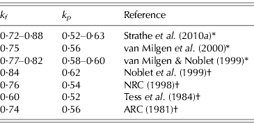
* Partial efficiencies derived from multivariate modelling approaches.
† Partial efficiencies derived from the factorial approach (multiple linear regression).
Convergence and model selection
Two chains were run with different initial over-dispersed values. To assess convergence, four formal convergence tests at the core of the convergence diagnostic and output analysis (CODA) package were used (Best et al. Reference Best, Cowles and Vines1995), which are the Geweke, Heidelberger–Welch, Raftery–Lewis and Gelman–Rubin diagnostic tools.
Statistics, such as the mean, median, percentiles and 0·95 credible interval (CrI) can be calculated from the samples making up the posterior distribution. The CrI is the Bayesian version of the traditional CI and it represents a non-parametric interval of the posterior distribution. In Bayesian methodology, a parameter is considered a random variable and thus the CrI may be interpreted as the 0·95 probability that the parameter lies within the interval (lower–upper) given the observed data and prior distribution (Gelman et al. Reference Gelman, Carlin, Stern and Rubin2004). In Bayesian analysis, there is no standard model selection/reduction criterion such as the likelihood ratio test. In the current analysis, three criteria for model selection were used. Firstly, a reduction in the residual variance for three response variables fitted to the two sets of equations. Secondly, the precision of the estimated parameter/effect, which is judged by its 0·95 CrI and computation of the proportion of posterior samples that are different from zeros. This proportion may be interpreted similar to a P-value of the underlying hypothesis in traditional statistics. Thirdly, the Deviance Information Criteria (DIC), which is a general tool to assess the trade-off between model fit (deviance: −2 log likelihood) and complexity (number of effective parameters) was used. The notion that ‘smaller is better’ is preserved in the DIC (Spiegelhalter et al. Reference Spiegelhalter, Best, Carlin and Van Der Linde2002). Differences of 5 and 10 DIC units are considered a tendency and a substantive improvement of fit to data, respectively (Spiegelhalter et al. Reference Spiegelhalter, Best, Carlin and Van Der Linde2002).
Prediction procedure
The prediction procedure in the current paper followed Bayesian modelling convention (Gelman et al. Reference Gelman, Carlin, Stern and Rubin2004) and used the observed data (Y) and posterior parameters (θ = [β i , kp, kf, b]T) obtained from the model estimation to make inferences about a predicted quantity Y p, e.g. PD. Hence, the distribution of Y p was obtained conditional on the observed data and the model parameter (i.e. the posterior predictive distribution of Y p) as
 $$p({\bf Y}_p \left| {\bf Y} \right.) = \int {\,p({\bf Y}_p |{\bf \theta} )p({\bf \theta} |{\bf Y}){\rm d}{\bf \theta}} $$
The first of the two factors in the integral is the MVN distribution for the future observations given the value of θ (Eqn (1)). The second factor is the posterior distribution of θ given the observed data. The posterior predictive distribution of Y p can thus be thought of as an average of the conditional predictions over the posterior distribution of θ. The integral in Eqn (6) is not analytically tractable, but it can be approximated by using Monte Carlo sampling from the posterior and summarize the samples in median and 0·95 CrI.
All models were implemented in the general purpose software for Bayesian modelling, WinBUGS (Lunn et al. Reference Lunn, Thomas, Best and Spiegelhalter2000).
RESULTS
Parameter estimates and their uncertainties are presented in Tables 3 and 4 for the two equation sets under two different prior settings. Both equation sets and both priors predicted the same MEI at various stages of growth as the parameter estimates were identical. The asymptotic MEI was estimated in the range of 44–48 MJ/day, which was not significantly different between genders (P > 0·05). Parameters (c, d, PDmax and BWPDmax) describing energy partitioning between PD and LD were unaffected by the different priors as the estimates were numerically identical and thus the representation of the prior setting was not important. Figure 1 presents the posterior predictive distribution of PD data with 0·95 CrI. Both models covered the observed variability in the PD data. However, equation set (3) provided a more realistic trend for the PD data, as PDmax occurred at later stages of growth, which suggests that the assumption of a linear decline in F may not hold when growth is studied from 25 to 150 kg BW. This was supported by a better fit to the data with equation set (3), i.e. a DIC of 637 v. 642.

Fig. 1. Posterior predictive distribution for PD (g/day) given by two different equation sets and three genders. The line represents the posterior median and the grey shaded area is the 0·95 CrI for the predictions.
Table 3. Parameter values estimated by equation set (2)* presented as posterior means and 0.95 CrI in parenthesis

* See Materials and methods section for details.
† Here a is ME requirement for maintenance, c is the fraction of ME for production (F) used for PD at 25 kg BW and d is the change in F per kg BW change. Parameters M and k can be interpreted as the asymptotic MEI and the fractional change in MEI due to a change in BW. Parameters k p , kf and b are the partial efficiencies and metabolic exponent parameter, respectively.
‡ Normal and uniform refer to the priors assigned to parameters b, k p and k f .
§ Deviance information criteria.
Table 4. Parameter values estimated by equation set (3)* presented as posterior means and 0·95 CrI in parenthesis

* See Materials and methods section for details.
† Here a is ME requirement for maintenance, maximum rate of PD is denoted by PDmax and the associated BW at that point BWPDmax. Parameters M and k can be interpreted as the asymptotic MEI and the fractional change in MEI due to a change in BW. Parameters k p , kf and b are the partial efficiencies and metabolic exponent parameter, respectively.
‡ Normal and uniform refer to the priors assigned to parameters b, k p and k f .
§ Deviance information criteria.
The estimates of the maintenance requirement (a, MJ ME/(kg BWb × day)) were dependent on the specification of the prior distributions, and the uniform distribution produced lower point estimates of a (Tables 3 and 4). ME maintenance requirement point estimates ranged from 0·83 to 0·96 MJ ME/(kg BWb × day) and they were highly correlated to estimates of b, k p and k f . These parameters did not change much from their prior location of 0·60, 0·60 and 0·80, respectively, but their precision increased because the standard errors (s.e.) were reduced by two-thirds, i.e. s.e. ≈ 0·1 (prior) v. s.e. ≈ 0·03 (posterior). Hence, the estimates of a, b, k p and k f derived here were not unique as they were dependent on the setting of the priors and thus they should be interpreted with caution. Moreover, gender-specific maintenance requirements should be reduced to a single parameter. Parameter estimates and CrI given in Tables 3 and 4 showed that barrows and gilts could not be separated, and hence these groups were combined in the further analysis resulting in two groups, i.e. boars and barrows + gilts. The DIC statistic for the two reduced models (Table 5) resulted in simpler models that were obtained by grouping barrows and gilts. The associated DICs were 633 and 626 for the reduced versions v. DICs of 642 and 637 for the original versions of equation sets (2) and (3). Still, equation set (3) was the preferred model, i.e. a DIC of 626.
Table 5. Parameter values and 0·95 CI in parenthesis estimated by two different equation sets*. Parameter contrasts are computed for boars against barrows + gilts

* See Materials and methods section for details.
† Here c is the fraction of ME for production (F) used for PD at 25 kg BW and d is the change in F per kg BW change. Parameters M and k can be interpreted as the asymptotic MEI and the fractional change in MEI due to a change in BW. Maximum rate of PD is denoted by PDmax and the associated BW at that point BWPDmax.
‡ The proportion of posterior samples that are different from zero computed for the contrast boars against barrows + gilts.
Parameter values obtained by fitting the reduced models to data and use normal priors are presented in Table 5 for the two equation systems. Parameters describing energy partitioning above MEM between PD and LD in equation set (2) were not statistically different between the two groups as posterior probabilities for the expressions c boar −c barrow+gilt > 0 and d boar −d barrow+gilt > 0 were 0·24 and 0·10, respectively. A large numerical difference was observed, as boars partitioned 5% more of MEG towards PD at 25 kg BW. In general, energy was diverted from PD towards LD with increasing BW because estimates of d for both groups were significantly different from zero (P < 0·05). Evaluation of PDmax values estimated by equation set (3) suggests that the boars deposited more protein (P < 0·001), i.e. 250 g/day (0·95 CrI: 237–263) v. 210 g/day (0·95 CrI: 198–220). Furthermore, the PDmax was reached at later stages of growth in boars because BWPDmax was 109 kg (0·95 CrI: 93·6–130) for boars and 81·7 kg (0·95 CrI: 75·6–89·5) for barrows and gilts. The quantity F was suggested here as a measure of the priority for PD in energy terms. Hence, a contrast in F between boars and the combination of barrows and gilts was computed at different stages of growth (Fig. 2). Although F was related non-linearly to BW in equation set (3), both equation sets estimated the numerical difference between the two groups to be c. 5–6% at 25 kg BW increasing to c. 10–11% at 150 kg BW. Moreover, boars partitioned significantly more ME above MEM towards PD c. 50–60 kg BW as the 0·95 CrI did not overlap zero, which was also shown in both equation systems.

Fig. 2. Posterior predictive distribution for the comparison between boars and barrows + gilts in their priority for PD computed at different stages of growth. The quantity (F boars−F barrows + gilts) describes the difference between the two groups in the fraction of ME above maintenance allocated for PD as estimated by two different equation sets. The line represents the posterior median and the grey shaded area is the 0·95 CrI for the predictions.
DISCUSSION
MEI
Similar to the current study, the ARC (1981) and the NRC (1998) used asymptotic equations to relate energy intake to BW. Figure 3 presents the posterior predictive distribution for MEI (MJ/day) plotted as a function of BW. The line represents the posterior median and the grey shaded area is the 0·95 CrI for the predictions. The plot shows clearly that adopting an asymptotic function was justified, but MEI was c. 10–15% less in the current study compared with those reported by the ARC and NRC (assuming 0·95 ME to DE ratio). The experiment was conducted in metabolism cages, which may reduce feed intake compared to that measured when pigs are housed individually in pens. Therefore, care should be taken when extrapolating the current results to other situations, although it should be noted that most modern genotypes will probably consume less than those reported by ARC (1981) and NRC (1998).

Fig. 3. Posterior predictive distribution for MEI (MJ/day) plotted as a function of BW. The line represents the posterior median and the grey-shaded area is the 0·95 CrI for the predictions.
None of the previous multivariate approaches used to analyse PD and LD data included simultaneous modelling of MEI (van Milgen & Noblet Reference van Milgen and Noblet1999; Strathe et al. Reference Strathe, Danfær, Chwalibog, Sørensen and Kebreab2010a ). Moreover, measured MEI in the preceding studies was used as an independent variable and assumed to be free of error. Some consequences of ignoring measurement error include masking important features of the data, losing the power to detect relationships among variables and introducing bias in function/parameter estimation (Carroll et al. Reference Carroll, Ruppert, Stefanski and Crainiceanu2006). The severity of the problem depends on the magnitude of error in the independent variables. Dhanoa et al. (Reference Dhanoa, Sanderson, Lopez, Dijkstra, Kebreab, France and Ortigues-Marty2007) presented alternative regression approaches to the ordinary least square for modelling energy components; however, their study was concerned with estimating k g (efficiency of utilizing ME for energy gain) and MEM, which were derived from regressing energy gain on MEI. Their results showed that accounting for measurement error in MEI increased both k g and MEM, suggesting that these parameters were biased downwards when the ordinary least squares method was used (Dhanoa et al. Reference Dhanoa, Sanderson, Lopez, Dijkstra, Kebreab, France and Ortigues-Marty2007). The functional forms that were utilized in the present study were non-linear, and therefore ‘classical’ regression models were not applicable. Shortcomings of multiple linear regression models have been covered by Koong (Reference Koong1977) and van Milgen & Noblet (Reference van Milgen and Noblet1999), including reversion of the relationship between responses (PD and LD) and driver (MEI) and statistical issues related to collinearity between independent variables. Use of Markov Chain Monte Carlo (MCMC) techniques for parameter estimation in these complex models was straightforward, and hence measurement error in the determination of MEI could be modelled. The BW variable was assumed to be free of error, which is a realistic assumption as measurement error in the determination BW is small as fluctuations in BW over time are animal driven, i.e. ‘animal intrinsic variability’ (Strathe et al. Reference Strathe, Sørensen and Danfær2009, Reference Strathe, Danfær, Nielsen, Klim, Sørensen, Sauvant, van Milgen, Faverdin and Friggens2010b ) and hence, utilizing the measured value can be justified. It would be straightforward to include BW as a fourth trait in the recursive equations, modelling the growth curve, but then several more parameters would have to be estimated and therefore it was decided not to do this in the current study.
Partitioning of MEI into protein and lipid
Published estimates of the maximum PD for growing pigs vary considerably from c. 80 to more than 200 g/day. Tauson et al. (Reference Tauson, Chwalibog, Jakobsen and Thorbek1998) investigated PD patterns in boars of three breeds (Landrace, Duroc and Hamshire, Danbred lines) and found that the breeds differed in the capacity for PD, with Duroc and Hampshire being superior to Danish Landrace boars. These Duroc and Hampshire boars of high genetic potential had a capacity for PDmax of c. 227 g/day and there was a significant quadratic relationship between PD and metabolic BW, showing that the shape of the PD curve was non-linear. These results agree well with the current results. In a later study, litter mates were serially slaughtered, and a preliminary analysis of these data has been presented by Danfaer & Strathe (Reference Danfaer, Strathe and Bach Knudsen2012). The barrows and gilts in that study reached their PDmax at c. 120 days of age, whereas the boars’ PD rate continued to increase until c. 150 days of age. The predicted maximum rates of PD were 229, 197, 186 g/day at 113, 79 and 80 kg BW for boars, gilts and barrows, respectively. The small discrepancies between the results on PDmax from Tauson et al. (Reference Tauson, Chwalibog, Jakobsen and Thorbek1998), from the present study and those obtained from the serial slaughter study can be explained by differences in experimental methodology. It is well documented that the N balance technique overestimates the amount of PD because the deposition is calculated as the remainder after correcting for N loss in urine and faeces. These two components are more likely to be under- than overestimated, and hence the N balance tends to be overestimated (e.g. Quiniou et al. Reference Quiniou, Dubois and Noblet1995).
With increasing BW, an increasing part of MEI above maintenance will be designated towards LD for the three genders as the parameter d > 0, i.e. energy partitioned towards PD declined linearly with increasing BW. van Milgen & Noblet (Reference van Milgen and Noblet1999) reported that lean genotypes partitioned 0·49 of ME above MEM towards PD at 20 kg BW, which agrees well with the current estimates (Table 5). In addition, van Milgen & Noblet (Reference van Milgen and Noblet1999) observed that extremely lean boars maintained a constant partitioning of energy within the observed BW range (20–100 kg). This could not be confirmed in the current study, perhaps due to the limited amount of information between 25 and 75 kg BW.
Utilization of prior information
In the current data analysis, informative prior distributions for parameters b, k p and k f were used and this gave numerical information crucial for estimation of the model. The priors were derived from earlier data analysis and hence represented the traditional way of using priors in the Bayesian framework. In addition, the prior distributions used in the current study did not supply any controversial information, but were strong enough to pull the data away from biologically inappropriate inferences, which might have been consistent with the likelihood (Strathe et al. Reference Strathe, Dijkstra, France, Lopez, Yan and Kebreab2011). However, care also needs to be taken in implementing these analyses to account for biologically supported parameter spaces, because consideration must be given to whether the pig population in the new dataset resembles the population(s) from which the prior information is borrowed – for example, priors for parameters describing PD potential should be not be taken from Meishan pigs when aiming at modelling PD data from Pietran pigs.
The prior information in the current study was structured into two different proper prior distributions, for purposes of sensitivity analysis, which is an important part of Bayesian analysis (Gelman et al. Reference Gelman, Carlin, Stern and Rubin2004). It was shown that only the ME requirement for maintenance was sensitive to the statement of prior belief. The final estimate of the maintenance component 0·91 MJ ME/(kg BW b × day) (0·95 CrI: 0·78–1·09) should be interpreted with caution. Nonetheless, introduction of prior information in the data analysis eases comparison with literature values for maintenance requirements in growing pigs and the final estimates were similar to those reported by van Milgen & Noblet (Reference van Milgen and Noblet1999) for lean meat-type pigs. An older Danish investigation reported an ME requirement for maintenance to be 0·93 MJ ME/(kg BW0·60 × day) (Just et al. Reference Just, Jørgensen and Fernández1983), which aligned very well with the current estimate(s).
The Bayesian framework enables the development of robust probabilistic analysis of error and uncertainty in model predictions by explicitly accommodating measurement error, parameter uncertainty and model structure imperfection. The current analysis presents a Bayesian formulation for simultaneous calibration of an energy-based pig growth model, with prior precisions of model parameters, data collected, measurement error or inter-animal variability. The model was developed initially within the statistical framework presented by Strathe et al. (Reference Strathe, Danfær, Chwalibog, Sørensen and Kebreab2010a ), but it was noted that parameter solutions were sensitive to the starting values provided to the routine. This was discovered by means of a grid search and hence it was decided not to report these results for comparison. The intent was to illustrate how this novel approach can be used to transfer knowledge in time (i.e. past to present), and therefore used to calibrate an energy-based pig growth model to sparse data, collected in an intensive metabolic study. Moreover, it was illustrated that the analysis was strengthened through integration of prior knowledge in the modelling process. Finally, it must also be noted that the value of the Bayesian modelling approach increases with the complexity of the structural model.
CONCLUSION
Bayesian framework is a tool well-suited to modelling MEI, PD and LD curves, when these traits are considered as dependent variables. Utilization of prior knowledge could be used directly in the data analysis, which may be important when sparse datasets are analysed due to issues related to parameter identifiability. The concepts presented in the current paper may be extended to form the basis of a complete nutritional pig growth model in which all parameters are expressed in terms of distributions that can be updated/calibrated using MCMC methods.
Funding from the Pig Research Centre, Denmark and the Sesnon Endowed Chair Fund (UC Davis) is acknowledged.


