


Introduction
Beef cow culling can be defined as the removal of selected beef cows from the herd permanently. Culling decisions, i.e., the selection and timing of cows to cull, are an essential part of farm management to sustain profitability and productivity of the herd in the short run and long run. According to United States Department of Agriculture (USDA) data, the culling rate (the percentage of cows removed permanently from herd each year) was 12.9% in all operations and 18% in small operations where herd size is 1–49 cows in 2017 (USDA National Animal Health Monitoring System, 2020). Studies estimate the revenue generated from cull cow sales to be about 15–30% of yearly revenue (Amadou et al., Reference Amadou, Raper, Biermacher, Cook and Ward2014; Blevins, Reference Blevins2009; National Cattlemen’s Beef Association, 2016). The reasons for cow culling are related to both biology and economics. Reproductive efficiency including pregnancy status and other fertility problems, age, disposition, cow’s health and physical soundness, concerns of producing inferior calves, and a desire for genetic improvement from replacement breeding stock are primary biological reasons to cull a cow (Arnold, Burris, and Townsend, Reference Arnold, Burris, Townsend, Arnold, Burris and Townsend2021; Hersom, Thrift, and Yelich, Reference Hersom, Thrift and Yelich2018). In addition to cow health and herd structure, cow-calf prices and seasonal trends in the markets, production costs including maintenance and replacement heifer costs, expected future earnings, cash flow, and risk management are major economic factors that affect culling decisions (Hersom, Thrift, and Yelich, Reference Hersom, Thrift and Yelich2018; Peel and Doye, Reference Peel and Doye2017; Ward and Powell, Reference Ward and Powell2017). Therefore, ranchers and farm managers can improve both profitability and productivity of the herd by utilizing a data-driven and informed culling strategy.
There is an extensive literature analyzing the reasons and motivation behind beef cow culling and evaluating optimal culling strategies under a variety of assumptions (Azzam and Azzam, Reference Azzam and Azzam1991; Bentley, Waters, and Shumway, Reference Bentley, Waters and Shumway1976; Boyer, Griffith, and DeLong, Reference Boyer, Griffith and DeLong2020; Frasier and Pfeiffer, Reference Frasier and Pfeiffer1994; Ibendahl, Anderson, and Anderson, Reference Ibendahl, Anderson and Anderson2004; Mackay et al., Reference Mackay, Whittier, Field, Umberger, Teichert and Feuz2004; Melton, Reference Melton1980; Tronstad and Gum, Reference Tronstad and Gum1994). Although pregnancy check is not common in the U.S. (USDA National Animal Health Monitoring System, 2020), as parallel to some of these study’s conclusions, culling open cows immediately after pregnancy check is advised in practice. However, the literature has mixed conclusions and underlines the impact of fertility rates, age of open cows, prices, and costs on the optimal culling strategies that may improve herd productivity and provide a flexible strategy to cope with price cycles and costs.
This study develops a dynamic linear programing model designed for cow-calf operations in the U.S. to determine optimal beef cow culling age and measures the sensitivity of the optimal strategies to other factors such as cow’s fertility, cow-calf prices, variable costs, and replacement prices. The model is solved with the data obtained for a spring calving herd that sold weaned calves in the fall in Kentucky, which is largely representative of the South. In addition to the methodological contributions, this research aims to provide practical guidance for beef cattle producers.
Literature review
The economics of culling decisions on cow-calf operations in the U.S. has been analyzed considering various aspects in the literature for decades. The majority of studies that specifically focus on the optimal culling age employed a net present value framework by either comparing the opportunity cost between retaining a cull cow and replacing with a bred heifer, or evaluating the contribution of cow to herd future revenue streams throughout the productive years of the cows (Bentley, Waters, and Shumway, Reference Bentley, Waters and Shumway1976; Boyer, Griffith, and DeLong, Reference Boyer, Griffith and DeLong2020; Ibendahl, Anderson, and Anderson, Reference Ibendahl, Anderson and Anderson2004; Mackay et al., Reference Mackay, Whittier, Field, Umberger, Teichert and Feuz2004; Melton, Reference Melton1980; Trapp, Reference Trapp1986). These studies based their models on variations of asset replacement methodology discussed in Burt (Reference Burt1965) and Perrin (Reference Perrin1972). Azzam and Azzam (Reference Azzam and Azzam1991) and Frasier and Pfeiffer (Reference Frasier and Pfeiffer1994) worked with Markovian multi-stage decision analysis with transition probabilities of different states including cow’s age, productivity, calving season, body condition scores, and calving dates. Dynamic programing has also been applied to find the optimal decision rule to cull a cow (Tronstad and Gum, Reference Tronstad and Gum1994).
The literature on culling versus keeping open cows has been mixed. Several studies have suggested that all open cows should be culled. In their Markovian decision analysis, Azzam and Azzam (Reference Azzam and Azzam1991) used cow’s productive status (open, pregnant, and unsound) in combination with cow’s age (2.5–10.5) and two calving seasons (spring and fall) for Nebraska as transition states and two decisions (keep and replace). They recommended replacing all open cows with spring-born heifers and retaining any pregnant cows of any age. Using a similar methodology augmented with the impacts of herd management practices, Frasier and Pfeiffer (Reference Frasier and Pfeiffer1994) also suggested culling all open and late lactating cows. Their sensitivity analysis underlined the impact of different cow and calf prices and replacement heifer cost on the optimal culling strategies. The most recent study on the optimal culling decisions, Boyer, Griffith, and DeLong (Reference Boyer, Griffith and DeLong2020) worked with Tennessee herd level data for both spring and fall calving seasons and analyzed the impact of productivity failure (missing a calf during the production life) on the operation’s long-term profitability. They concluded that selling an open cow after missing one calf would be a better option to increase the profitability instead of retaining and rebreeding the cow.
The literature that has left the door open to retention has focused on the calving system, varying fertility of cow across ages, genetic improvement, the importance of prices, and replacement costs in this determination. Bentley, Waters, and Shumway (Reference Bentley, Waters and Shumway1976) found the optimal replacement policy to be replacing a cow after her seventh calf is sold since the expected present value of the cow is maximized at age 8. In their sensitivity analysis, they conclude that changing cattle prices and feed costs does not impact the optimal policy. They demonstrated that culling decisions are sensitive to lower calving rates and changing cull cow prices with carcass quality (i.e., lower prices for older cows), which lead to an earlier optimal culling. Melton (Reference Melton1980) investigated the impact of an endogenous genetic progress in the herd on the optimal culling age with experimental herd data in Florida. Results suggested a culling age of 8 under genetic improvement and 11 without genetic progress. Tronstad and Gum (Reference Tronstad and Gum1994) performed a stochastic dynamic programing model with biannual calving, cow fertility estimates, and stochastic prices under a multi-period horizon with the objective of maximizing expected wealth. Their model results emphasized that a dual calving system would be more profitable for ranchers. They also utilized a Classification and Regression Trees (CART) technique to provide more practical and interpretive culling advice based on dynamic programing model results. Their decision trees included “keep” and “replace” decisions and were based on 1,100 combinations of state variables (cow age, pregnancy status, calf price, replacement price, and cull cow prices) used in the model. Their tree-based analysis identified age for open cows and calf prices for pregnant cows as the most important variable in culling. CART results also rejected the culling strategy which suggests culling open cows all the time regardless of their productivity and stated that when spring and fall calving are possible that would make rebreeding possible, open cows should be kept 26% of time. The retention rate was found to be 95% for pregnant cows in the study.
One of the early studies evaluating the impact of prices on the culling decisions and herd decomposition, Trapp (Reference Trapp1986) assumed a varying herd size and nonconstant prices in a simulated herd model and pointed out a flexible culling strategy with culling ages varying from 5 to 12 to manage cyclical prices. Mackay et al. (Reference Mackay, Whittier, Field, Umberger, Teichert and Feuz2004) discussed the impact of prices on marketing strategies based on analysis using data from a Nebraska cow-calf operation. They pointed to the changing herd decomposition under different prices; an older herd was better when prices were lower, and a younger herd was better when prices were higher. Ibendahl, Anderson, and Anderson (Reference Ibendahl, Anderson and Anderson2004) studied the optimal culling policy within a net present value framework with fertility data obtained from Tronstad et al. (Reference Tronstad, Gum, Ray, Rice, Tronstad, Gum, Ray and Rice1993). They contradicted the conclusion of the studies which has been to cull open cows by focusing on the age of open cows and suggested a flexible culling strategy to deal with production costs. They emphasized the impact of replacement and production costs on the replacement decisions and recommended retaining younger open cows when calf crop value and production costs are low and the difference between replacement heifer cost and cull value is high.
The culling rate is about 30% in dairy operations (USDA National Animal Health Monitoring System 2020) and culling strategies have been examined with a focus on the cow performance and milk production in the dairy literature (Cabrera, Reference Cabrera2010; Lehenbauer and Oltjen, Reference Lehenbauer and Oltjen1998; Van Arendonk, Reference Van Arendonk1986; Van Arendonk and Dijkhuizen, Reference Van Arendonk and Dijkhuizen1985). Van Arendonk and Dijkhuizen (Reference Van Arendonk and Dijkhuizen1985) studied optimal policies for open cows with a variation in the time of conception and three alternatives: inseminating, leaving her open, and culling her immediately. They underlined the impact of replacement costs on culling open cows. Cabrera (Reference Cabrera2010) applied a Markovian linear programing model with a net revenue maximization objective and solved the model with “keep” and “replace” decisions under different dietary treatments and state variables which are defined by parity, month in lactation, and pregnancy status. The model suggests that pregnant cows should be kept regardless of their production performance and higher culling rates should be allowed when milk prices and replacement costs are low and corn prices are high. Open cows are culled earlier depending on market conditions.
This study aims to build upon this literature by constructing a model framework for cow-calf operations in the U.S. to evaluate culling strategies. The objectives of the study are to evaluate optimal culling decisions with a base model and several experiments performed with a variety of assumptions related to cost, fertility, weights, and prices, to determine the conditions under which open cows should be retained and estimate the impact of pregnancy checking on herd profitability and culling decisions. In addition to its methodological contributions in applying an infrequently used programing technique ideally suited to the problem considered, it also has potential to provide practical guidance for beef cattle producers.
Methods and data
The economic decision-making framework of a commercial size beef cow-calf producer is formulated as a single-year dynamic linear programing model since cow culling decisions depend on the dynamic nature of changes in productivity by age of brood cow and stochastic factors (probabilities of pregnancy, cow death, calf loss, etc.). Optimal decision modeling of problems with such dynamic elements can be formulated with both multi-period and single period dynamic linear programing models. In multi-period models, the number of periods can be assumed to be known or unknown depending on the problem’s nature and research considerations and optimal solutions are generated with the assumption of disequilibrium where decisions vary over a number of time periods. Single period dynamic linear programing models which are also called equilibrium models, assume that optimal decisions are repeatedly made in all time periods and defined as long run steady-state solutions (McCarl and Spreen, Reference McCarl and Spreen1997). The model used in the study is a single-year steady-state equilibrium of unknown asset life with prices, costs, and probability values that is solved with results then being interpreted. The operation’s size is assumed constant by imposing a herd size constraint in the model formulation.
The dynamic linear programing model used in the study is specified as:

Max: Net Return above Selected Costs
 $$\sum _{y}\left(\sum _{p}{Prices}\left(p,y\right)\;{\rm *}\;Sale\left(p,y\right)-\,\sum _{c}{Production\;Cost}\left(c,y\right)\;{\rm *}\;Herd\left(c,y\right)\right)$$
Subject to:
Herd Size:
 $$\sum _{c,y}Herd\left(c,y\right)\leq 100$$
Market Balance
 $$Sale\left(p,y\right)-\sum _{c}{Fertility} \;{Probability}\left(c,p, y\right)\;{*\;Herd}\left(c,y\right)\leq 0\;\;\forall p,y$$
Linkage between ages:
Pregnant:
 $$\sum _{c}\left({Retention} \;{Probability}\left(c,'{Pregnan}t', y\right)\;{*\;Herd}\left(c,y\right)\right)-Herd\left(\mathit{'}\mathit{WithCalf}\mathit{'},y+1\right)\leq 0\;\;\forall y\lt 12$$
Open:
 $$\sum _{c}\left({Retention} \;{Probability}\left(c,'Open',y\right)\;{*\;Herd}\left(c,y\right)\right)-Herd\left(\mathit{'}\mathit{NoCalf}\mathit{'},y+1\right)\leq 0\;\;\forall y\lt 12$$
Cull:
 $$\sum _{c}\left({Fertility} {\;Probability}\left(c,'Cull', y\right)\;{*\;Herd}\left(c,y\right)\right)-\sum _{c}Herd\left(c,y+1\right)-Sale\left('Cull',y\right)\leq 0\forall y\lt 12$$
Where: y is the age (2 to 13 years old herein) of each cow. c is the index of three different types of cows depending on their pregnancy status: cow with calf at side from previous year (With Calf), cows with no calf from previous year (No Calf), and first-time heifer (two-year-old bred heifers). Two-year-old bred heifers are purchased to replace cull cows. p denotes the three different products which are being sold at the market: steer, heifer, and cull cows. k is the index of decisions of whether to keep a cow based on whether or not she calved in the previous year. Herd(c,y) is herd composition at the equilibrium solution (repeated optimal decisions as discussed above) and it indicates the number of cows of different ages that are raised in the operation after culling decisions are made in the model. It should be noted that Herd(c,y) is both a decision and an accounting variable in that the model chooses whether or not to retain a cow of a given status c of age y which in turn affects the number of cows of that status c that are of age y + 1. Sale(p,y) is an accounting variable reflecting the number of calves and cull cows that are sold under the equilibrium solution. Production Cost(c,y) includes annual variable cost per cow and ownership costs of a bred replacement heifer.
Equation 1, the objective function is to maximize the expected herd level net return above selected costs while equations 2–6 impose various constraints. A commercial operation herd size is assumed with a maximum of 100 cows allowed in equation 2. The herd size of 100 is selected to formulate a medium scale cow-calf operation (50 to 199 cows) and make results more interpretable in terms of percentages. Equation 3 assures market balance by limiting sales to the amounts produced for every cow age. Linkage equations (4–6) are age sequencing constraints which ensure that the number of cows c of age y + 1 must be less than or equal to number of that cow type that were kept until age y in a standard dynamic linear program fashion.
There are two probability series in the model: fertility and retention. Fertility Probabilities(c,p,y) are the chance of products p (having a steer, heifer, and live cow at year end) based on age y and prior year status c (cow with calf at side or a cow that failed to calve last year). Retention Probabilities(c,k,y) reflect the percentage of cows that have a calf at side or are not this year (after including the chance of her death or being unsound) and are available for retention to next year. Fertility and Retention probabilities given in Table 1 are calculated based on calving rates and fertility estimates obtained from Tronstad et al. (Reference Tronstad, Gum, Ray, Rice, Tronstad, Gum, Ray and Rice1993). The probability of calving, survival, and retention vary depending on the cow’s age and her productivity status in the previous year. For example, if a cow is 5 years old and had a calf at her side last year, she has a 76.5% chance of having a calf this year and a 96.6% chance of surviving after calving. The probability of this same cow calving again is 71.9% and the probability of her failing to calve is 22.0% (the first panel of Table 1). The fertility rates are lower for cows without calves from previous year (the second panel of Table 1). These cows are assumed to have either lost their calf or failed to calve in the previous season. On the other hand, if a cow of the same age did not have a calf at side last year, her chance of calving this year is 64.7% and her chance of surviving increases to 98.3%. She also has a lower probability (58.3%) to calve this year and higher probability (31.8%) to fail to calve again. The calving rate is assumed to be 97.8% for replacement heifers, which is high because they are assumed to be bred when entering the herd. Calf survival rate from birth to weaning is assumed to be 95.5% for all cows with 4.5% calf death loss (Strohbehn, Reference Strohbehn1994).
Table 1. Fertility and retention probabilities

Notes: Data in the table are calculated based on calving rates and fertility estimates obtained from Tronstad et al. (Reference Tronstad, Gum, Ray, Rice, Tronstad, Gum, Ray and Rice1993).
The price data is obtained from the USDA Agricultural Marketing Service (AMS) and is given in Table 2. The 10-year (2012–2021) arithmetic average of monthly October and November feeder steer, heifer, and cull cow prices were used in the study to account for fall sales for spring calving herds in Kentucky. Steer and heifer prices for medium and large frame size and #1–2 muscling calves are utilized. Prices per pound are also adjusted downward to account for the heavier calves (commonly referred as price slide). Steers and heifers from 5- to 10-year- old dams are assumed to be weaned and sold at an average weight of 600 and 550 lb respectively. The weights for other calves are adjusted based on dam’s age with Beef Improvement Federation (2018) data. Cull cow prices are estimated using historical USDA-AMS price data from the 80-85% boning cow category. Cull cow price per lb is assumed to be $0.62 per lb with an average cull cow weight of 1,200 lb. To adjust cull cow prices with respect to carcass quality across ages, breaking grade cull cow prices (for age 2) and lean grade cull cow prices (for age 13) are used as minimum and maximum prices and adjusted price data is computed by decreasing prices linearly from age 2 to age 13. It is worth noting that two-year-old females may sell for higher prices since they are still under 30 months of age.
Table 2. Calf weights and prices

Note: Author’s calculations based on data obtained from USDA Agricultural Marketing Service and Beef Improvement Federation (BIF, 2018).
Annual cost per cow by age is computed for a spring calving herd and it covers annual variable costs, interest costs, and bred replacement heifer prices. Annual variable costs are obtained from Halich, Burdine, and Shepherd (Reference Halich, Burdine and Shepherd2022) and are shown in Table 3. These estimates are made for a spring calving cow-calf operation in 2021 and include only cash costs for the operation. The pasture stocking rate is assumed to be 2.0 acres per cow and hay consumption is assumed to be 2.5 tons per cow. The operation has its own pastureland and produces its own hay. Since operation costs presented in Table 3 may vary by herd size and management, an annual variable cost experiment is implemented to account for different annual cost per cow values and their impact on optimal culling strategies. Breeding costs are excluded from replacement heifers’ annual variable cost as they are purchased already bred. Opportunity cost of capital is estimated by using a 3% rate based on the value of breeding stock in inventory. Cow value declines by age in a straight-line fashion assuming the $1,500 bred heifer has 11 productive years and $700 cull cow ending value.
Table 3. Annual variable costs

Source: Halich, Burdine, and Shepherd (Reference Halich, Burdine and Shepherd2022).
The model timeline constructed for the spring calving herd based on common practices in the South is presented in Figure 1. The model starts in October at production year t after all calves were weaned and sold in weaning season of production year t-1 and ends in September. Therefore, there are no calves from the previous calving season during the model period and calf crops born are sold in the following weaning season.

Figure 1. Model timeline (spring calving system).
The base model is a single-year steady-state equilibrium of unknown asset life with base prices, costs, and probability values that is solved with results then being interpreted. Various experiments are conducted to analyze the study objectives by resolving the model after changing relevant coefficient values. This allows for the evaluation of the robustness of the model and performance of a sensitivity analysis by comparing experiment results to those of the base model.
Results and discussion
The base model results can be seen in Tables 4 and 5 and suggest that producers should cull all cows that are older than 10 based on their productivity, production costs, and price assumptions made. This result reflects the reproductive performance of the cows that is maximized between age 4 and 9 and starts to decline after age 10 (Arnold, Burris, and Townsend, Reference Arnold, Burris, Townsend, Arnold, Burris and Townsend2021; Ward and Powell, Reference Ward and Powell2017). The operation makes a modest net return above specified costs of $12,347 and purchases 15.6 bred replacement heifers annually. The 100-cow operation consists of 70.7 cows with calves at their side, 15.6 first-time heifers, and 13.8 cows that failed to wean a calf. The model assumes that culling decisions are made at weaning time which is common for operations that do not incorporate pregnancy checking into their management. Results suggest culling cows that did not calve at age 7 and cows with calf at side at age 10 given their productivity status and probabilities. Each year, the operation sells 36.8 steers, 36.8 heifers, and 12.6 cull cows in the base model. The average cow age in the herd is 5 years and the average age of cows culled is 7.7 years with a 12.6% culling rate in the base model. Since the model developed in the paper is a single-year steady-state equilibrium model, the optimal culling decisions are repeated every year, and the herd composition is the optimal ending herd composition rather than the year-by-year path leading to the specified herd composition. These results are consistent with the literature which suggests the optimal culling age between 7 and 11 (Bentley, Waters, and Shumway, Reference Bentley, Waters and Shumway1976; Mackay et al., Reference Mackay, Whittier, Field, Umberger, Teichert and Feuz2004; Melton, Reference Melton1980; Trapp, Reference Trapp1986; Tronstad and Gum, Reference Tronstad and Gum1994).
Table 4. Optimal culling strategies: net return above selected costs and culling age
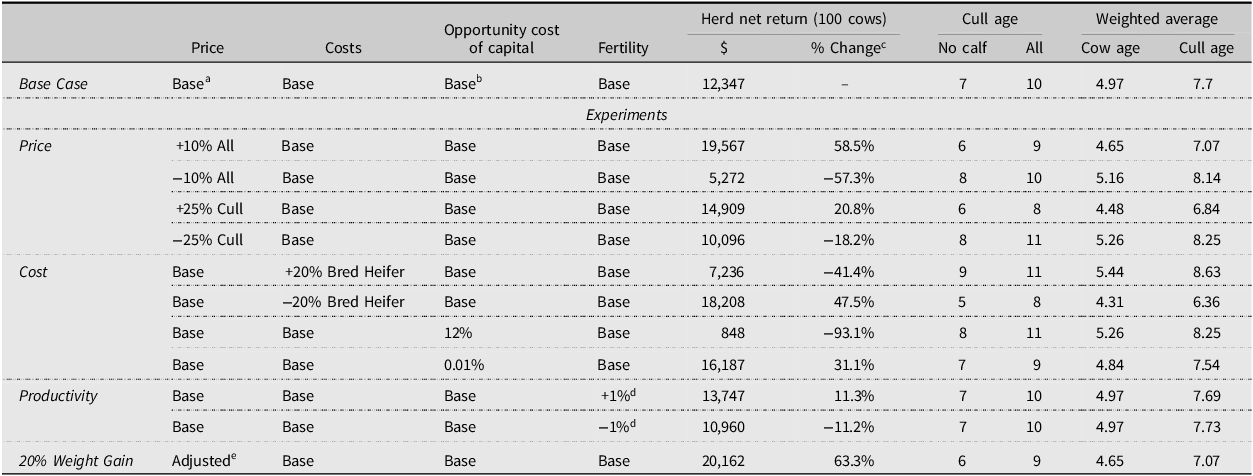
Notes: aSteer and heifer prices are age adjusted and cull prices are same for all ages.
bRate is 3% in the base model.
cChange from net return in the base case.
dPregnant, live calf: 1% for age 2–12 and 0.4% for age 13 & open to pregnant: 1%.
eSteer and heifer prices are adjusted.
Table 5. Optimal culling strategies: herd composition and sales
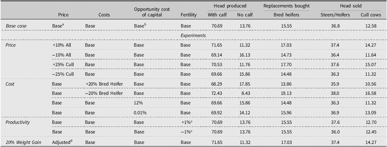
Notes: aSteer and heifer prices are age adjusted and cull prices are same for all ages.
b Rate is 3% in the base model.
c Pregnant, live calf: 1% for age 2-12 and 0.4% for age 13 & open to pregnant: 1%.
d Steer and heifer prices are adjusted.
Sensitivity analysis
To measure the sensitivity of these findings, several experiments are run with different prices, costs, fertility values, and genetic improvement resulting in weight gain. A pregnancy check experiment is also run to estimate the impact of pregnancy checking on the returns. The experiments’ outcomes underline the sensitivity of the optimal strategies to market conditions, cost structure, cow fertility, calf weights, and pregnancy check use (Tables 4–7). Several experiments are also run with different prices, costs, and fertility values to analyze the sensitivity of the optimal culling strategies to simultaneous changes in model components. Selected experiments are displayed in Table 6. The results show that producers enjoy favorable conditions where product prices and cow fertility are higher and production costs are lower. In addition to increases in net returns, herd structure also changes, and herd gets younger compared to the base model. That being said, optimal culling age and herd structure do not change under the experiments with adjusted cull cow prices by age (to account for decreasing carcass quality as cows get older) and simultaneous price changes in calf and replacement heifer prices (to reflect the price transmission between calf and replacement heifer markets). Changing the annual variable cost assumption also does not impact the optimal culling age, herd composition, or sale amount. This was an expected outcome since annual variable costs are assumed to be same across cow ages. These three experiments cause changes only in net return above selected costs comparing to base model results.
Table 6. Optimal culling strategies: multi-factor sensitivity analysis- selected experiements

Notes: aSteer and heifer prices are age adjusted and cull prices are same for all ages.
bRate is 3% in all models.
cChange from net return in the base case.
dPregnant, live calf: 1% for age 2–12 and 0.4% for age 13 & open to pregnant: 1%.
Table 7. Optimal culling strategies: pregnancy check

Prices
To evaluate the impact of different price assumptions on the optimal culling strategies, all output prices were changed by 10%. As expected, a simultaneous 10% increase in cow and calf prices enhances steer and heifer calf values, leading to a suggestion that producers should cull cows that did not calve and are older than 6 (one year sooner than the base model) and cull all cows older than 9. As shown in Table 5, calf sales rise to 74.8, the number of cows with calves at side increases to 71.6, and the number of cows without calves decreases to 11.3. On the other hand, a 10% decrease in prices favors a strategy of culling later at age 8 for cows that failed to calve. The optimal culling age for all cows is the same as the base model but the production amount is higher. This is a rational behavior since producers can take advantage of good market conditions and sell their calves and less productive cows, specifically by culling earlier when prices are high and keeping their cows and calves when prices are low. These results are consistent with Mackay et al. (Reference Mackay, Whittier, Field, Umberger, Teichert and Feuz2004) and Trapp (Reference Trapp1986) who pointed to the varying herd decomposition with prices.
To examine the impact of cull cow prices on decision variables, the model is run with a 25% increase only in cull cow prices. The results show a 20.8% increase in expected net return and the optimal strategy becomes culling cows with calves at their side at age 8 and those without calves at age 6. As expected, a stronger cull cow market encourages an earlier culling strategy. The experiment with the same amount of decrease in cull cow prices suggests a later culling strategy in which the optimal culling age is 8 for cows that did not calve and 11 for all cows. These results underline the correlation between cull cow prices and culling age.
Costs
The model includes three cost components: variable production costs, replacement heifer purchase price, and interest costs. Cost experiments for each component are performed separately to assess their individual impacts on culling decisions. Although the experiment with annual variable costs does not alter optimal culling decisions, the optimal culling strategy in the base model is highly sensitive to ownership costs of bred replacement heifers which includes both heifer value and opportunity cost of capital. Replacement heifer costs are a major part of operation costs for those producers who prefer to purchase a replacement heifer instead of raising it in the operation (Halich, Burdine, and Shepherd, Reference Halich, Burdine and Shepherd2022). When replacement is costly, producers tend to keep cows longer despite their declining productivity.
A 20% increase in replacement heifer value leads to a culling age of 11 for cows with calf at side and 9 for cows without calves. The same percentage decrease in replacement heifer values suggests an optimal culling of cows with calves at their side at age 8 and cows without calves at age 5. These are the largest changes in optimal age among all experiments performed. The average cow age in the herd is 4.3 years and the average age of cows culled is 6.4 years with a 16.6% culling rate when replacement heifer prices decrease by 20%. Producers buy 13.9 bred heifers each year when replacement heifer value increases by 20% and 19.1 replacement heifers when replacement heifer value is 20% cheaper compared to the value in base model.
Opportunity cost of capital changes also affect results by changing optimal culling age, net return, and herd structure. A 12% rate which makes replacement heifer purchases more costly for the producer, results in a later culling age of 8 for cows without calves and age 11 for all cows. The herd becomes older with an average cow age of 5.3 years.
Fertility
Cow’s genetics, body condition, and age are major determinants of reproductive efficiency and can be improved by appropriate management practices (Corah and Lusby, Reference Corah and Lusby2000; Tronstad et al., Reference Tronstad, Gum, Ray, Rice, Tronstad, Gum, Ray and Rice1993).
The selection of better replacement heifers, improvement of health and nutrition programs, and adoption of advanced technologies in fertility assessment and improvement can lead to more productive beef cows in the herd (Moorey and Biase, Reference Moorey and Biase2020). The model is also solved under different productivity values to see the impacts of enhanced management on optimal culling decisions. To this end, the probability of a cow that failed to calve becoming to be pregnant in the next year is changed by 1% across all ages, and calving rate is changed by 1% for age 2–12 and 0.4% for age 13. An increase in calving rate and fertility rates of 1% generates an additional 11.3% net return above specified costs and a similar optimal culling strategy of herd composition with same ages but higher sale amounts and culling rates compared to the base model’s outcomes.
Weight gain
An experiment is also run to measure the impact of calf weights on the optimal culling strategy. Steer and heifer weights are increased by 20% over the base model. Prices per pound are also adjusted downward to account for the heavier calves. A 20% increase in calf weights results in a considerable change in net return with a younger herd and an early culling strategy. The optimal culling age moves to 6 for cows that did not wean calves and 9 for cows that did wean calves. The operation sells 37.4 steers, 37.4 heifers, and 14.3 cull cows.
Pregnancy check
Although pregnancy checking is generally advised, it is not common among U.S. beef operations. According to USDA National Animal Health Monitoring System (2020) data, the percentage of operations that regularly pregnancy checking their cows (palpation, blood test, and ultrasound) was 31.6 for all operations in 2017. The reasons are labor and time costs, test costs, and producers’ beliefs and habits. For these reasons, previous results have been based on the assumption that cows are not pregnancy checked and culling decisions are made when calves are sold. To estimate the impact of pregnancy checking on the optimal culling decisions, an experiment with pregnancy checking is run. In the experiment, the marginal cost of pregnancy check is assumed to be $10 per cow with $150 flat trip charge and annual variable costs in the base model are adjusted accordingly. Fertility data is recalculated for the experiment based on the results of pregnancy testing.
The base model, as defined by equations 1 –6 is modified to run the pregnancy checking use experiment. The model objective function, herd size, market balance, and cull cows’ linkage constraints are the same as in the base model. Pregnant and open cows’ linkage constraints are adjusted, and two additional constraints are added to the model:
Linkage between ages:
Pregnant:
 $$\eqalign{ & \sum _{c}\left({Retention} \;{Probability}\left(c,'{Pregnan}t', y\right)\;{*\;Herd}\left(c,y\right)\right)\cr & \quad-Herd\left(\mathit{'}\mathit{WithCalfTestPregnant}\mathit{'},y+1\right)-Herd\left(\mathit{'}\mathit{WithCalfTestOpen}\mathit{'},y+1\right)\cr & \quad\leq 0\;\;\forall y\lt 12}$$
Open:
 $$\eqalign{ & \sum _{c}\left({Retention} \;{Probability}\left(c,'Open',y\right){*Herd}\left(c,y\right)\right)-\cr & \quad Herd\left({'NoCalfTestPregnan}t',y+1\right)-Herd\left(\mathit{'}\mathit{NoCalfTestOpen}\mathit{'},y+1\right)\leq 0\;\;\forall y\lt 12}$$
Pregnancy Test Constraints:
With Calf:
 $$\eqalign{ & {PregConstProbabilities}\left({'WithCalfTestOpen},'{WithCalfPregRateCons}t',y\right)\cr & \quad {*\;Herd}\left({'WithCalfTestPregnan}t',y\right)- \cr & \quad {PregConstProbabilities}\left({'WithCalfTestPregnant},'{WithCalfPregRateCons}t',y\right) \cr & \quad {*\;Herd}\left({'WithCalfTestOpe}n',y\right)- \cr & \quad {PregConstProbabilities}\left({'WithCalfTestPregnant},'{WithCalfPregRateCons}t',y\right) \cr & \quad {*\;Sale}\left('Cull',y\right)\leq 0\;\;\forall y}$$
No Calf:
 $$\eqalign{ & {PregConstProbabilities}\left({'NoCalfTestOpen},'{NoCalfPregRateCons}t',y\right)\cr & \quad{*\;Herd}\left({'NoCalfTestPregnan}t',y\right)-\cr & \quad{PregConstProbabilities}\left({'NoCalfTestPregnant},'{NoCalfPregRateCons}t',y\right)\cr & \quad{*\;Herd}\left({'NoCalfTestOpe}n',y\right)-\cr & \quad{PregConstProbabilities}\left({'NoCalfTestPregnant},'{NoCalfPregRateCons}t',y\right)\cr & \quad{*\;Sale}\left('Cull',y\right)\leq 0\;\;\forall \,y}$$
With the incorporation of pregnancy check into the model, there are five different types of cows (index c) in the herd: cows that weaned calves are tested as pregnant, cows that weaned calves, but are not pregnant, cows without calves that tested as pregnant, cows that did not wean calves and are open again, and first-time heifer. Two-year-old bred heifers are not tested since they are purchased as bred heifers. The linkage equations (7–8) are modified versions of equation 4 and 5 and ensure that the number of cows c of age y + 1 must be less than or equal to number of that cow type that was kept until age y. Equations 9 and 10 are the pregnancy test constraints and balance the production and cull amounts after testing cows for every cow age to ensure proper ratios of pregnant cows. The cow is tested as pregnant or non-pregnant and culled after the pregnancy test.
The results are presented in Table 7. The model results suggest that producers should keep cows that are weaning a calf and pregnant until age 13 and cull all cows without calves that are open. To be clear, the latter are cows that are essentially open back-to-back years. This indicates that a producer is better off starting with a cow that is already confirmed to be pregnant each year, and replacing those that are not pregnant with a bred heifer. Based on the herd decomposition following pregnancy checking, the model only keeps cows that did not wean calves that are 4-year-old and younger and only if they tested as pregnant. Similarly, culling age was determined to be 3 years of age for cows that did have a calf at their side, but were not pregnant. The 100-cow operation consists of 73.1 cows with calves at their side tested as pregnant, 2.9 cows with calves at their side tested as open, 3.3 cows without calves that tested as pregnant, and 20.7 first-time heifers. The average cow age in the herd is 4.24 years and the average age of cows culled is 6 years. The net return above selected costs increases by 68.2% compared to the base model because of the culling management changes enabled by pregnancy check information and increased calf sales (an additional $106.2 return per cow). Each year, the operation sells 44.9 steers (about 8 more than the base model), 44.9 heifers, and 17.3 cull cows (4.7 more than the base model) in the model.
Conclusion
Developing a culling strategy has great influence on financial and structural soundness of cow-calf operations and draws substantial attention from academics and extension field specialists. This study contributes to the current discussions with its methodology and results.
A single-year dynamic linear programing model is formulated and run with cow fertility estimates as well as price and cost data obtained for a spring calving herd in Kentucky to provide a set of culling strategies with optimal cow culling age for beef cattle producers. The initial base model assumed that all culling decisions were made at calf weaning/sale time, without the use of pregnancy testing. Results of the base model suggest that producers should cull all cows older than 10 and cows that fail to calve once they reach the age of 7. Given the base cost and price values, the 100-cow operation generates a net return above selected costs (mostly cash costs) of $12,347 and produces 70.7 cows with calves at their side, 15.5 bred replacement heifers and 13.8 cows that failed to wean a calf. Each year, the operation sells 73.6 calves and 12.6 cull cows. The average cow age in the herd is 5 years and the average age of cows culled is 7.7 years with a 12.6% culling rate in the base model.
The impact of each variable on the optimal decisions is also measured with several experiments to evaluate the sensitivity of the optimal strategy to changes in the markets, farm production costs, and management practices. The outcome of these experiments underlines the sensitivity of the optimal strategies to market conditions, particularly calf/cull cow prices, ownership costs of bred replacement heifer, and herd management skills to increase cow’s productivity and calf weights as essential parameters in optimal culling. While cow-calf price changes impact net return values to a considerable extent among experiments conducted, the cost sensitivity analysis with changing bred heifer replacement value alter both net return and herd age decomposition most substantially. Culling age in the base model (age 7 for cows that did not wean calves and 10 for cows with calves at their side) decreases to 5 for cows without calves and 8 for cows calves when replacement prices decrease by 20% and increases to 9 for cows without calve and 11 for cows with calves when replacement prices increase by 20%.
When pregnancy checking is incorporated into the model, net return above selected costs increased by 68.2%. This alone is noteworthy and occurs because the number of cows for which maintenance costs are incurred without the benefit of a calf in the following year is greatly reduced. Culling strategies also change as producers only keep cows without calves that are 4-year-old or younger and only if they are pregnant. No cows were kept that failed to wean a calf and also tested as open for the upcoming year. The cost of pregnancy testing was also important, which was assumed to be relatively low at $10 per cow, plus the $150 flat fee. This largely assumes that cattle were already being worked and can be thought of as the marginal costs of pregnancy checking.
One of the primary implications of the sensitivity analysis is that producers should pay a considerable amount of attention to management practices to monitor and improve cow’s productivity and calf weights since better management creates a potential to have lower number of open cows in the operation and earn higher net returns. The impact of higher weaning weights and increased probability of weaning calves results in substantive improvement in returns above the base model.
Data availability statement
Data and code are provided at Open Science Framework webpage and can be accessed from the link: https://osf.io/ery6x/?view_only=304a8fe855aa44cd89edbb172df8534f
Author contribution
Conceptualization, E.E., C.R.D., and K.H.B.; Data curation, E.E.; Formal analysis, E.E., C.R.D., and K.H.B.; Methodology, E.E. and C.R.D.; Software E.E. and C.R.D.; Validation, E.E., C.R.D., and K.H.B.; Writing – original draft, E.E.; Writing – review & editing, E.E., C.R.D., and K.H.B.
Financial support
This work was supported by Hatch Project no. KY004058 from the USDA National Institute of Food and Agriculture.
Competing interests
Erdal Erol, Carl R. Dillon, and Kenneth H. Burdine declare none.


 Open access