


1. Introduction
The use of food labels as marketing tools to distinguish products has become increasingly prevalent in recent years (McCluskey and Loureiro, Reference McCluskey and Loureiro2003). The increasing demand for local foods is one example, with state marketing programs such as New Jersey’s Jersey Fresh, Arizona’s Arizona Grown, and Oklahoma’s Made In Oklahoma branding efforts emphasizing products’ origins to capture the interest of state residents for in-state products. The marketing techniques employed by these state programs, some of which began in the 1980s, focus on promoting and improving the relationships between resident consumers and local food businesses within state borders. Previous studies have found large increases to in-state producer surplus from state promotion programs (Govindasamy et al., Reference Govindasamy, Schilling, Sullivan, Turvey, Brown and Puduri2004). Yet, consumers have varying definitions of “local,” and their proximity to state borders may or may not impact their definitions of “local.” According to the US Congress, locally grown constitutes food grown or produced within 400 miles, which in some cases could cover multiple states and/or territories (Martinez et al., Reference Martinez, Hand, Da Pra, Pollack, Ralston, Smith, Vogel, Clark, Lohr, Low and Newman2010).
The main goal of state branding programs, which have been established in every state (Onken and Bernard, Reference Onken and Bernard2010), is to use these improved relationships as a means to increase in-state producer income (Carpio and Isengildina-Massa, Reference Carpio and Isengildina-Massa2016). While these programs have the potential to benefit local food systems, they generally do not effectively measure their impacts or the cost-effectiveness of public funds used in these efforts (Hand and Clancy, Reference Hand, Clancy, King, Hand and Gomez2014). When assessing the effectiveness of these programs on consumer choices, out-of-state consumers are generally not included in the evaluations because most of the promotional techniques rely on motivating an in-state consumer’s state pride (i.e. the level of ethnocentrism that draws consumers to choose products promoting their respective states). However, consumers’ definitions of local are not necessarily tied to geo-political boundaries, and their relative preferences/values for regional-brand products or products from neighboring states within close proximity may not be significantly different from their preferences/values for in-state products. As noted in Neill et al. (Reference Neill, Holcomb and Lusk2020) excluding out-of-state consumers overstates willingness-to-pay estimates which leads to inaccurate policy recommendations. However, this result could be heterogeneous within each state depending on individuals’ distance to state borders and their respective level of state ethnocentrism.
The extensive literature on regional and local allegiances has muddled the expected response to varying geographical labeling schemes. Moreover, the tradeoffs between state and regional branding are difficult to parse out without having a better understanding of one’s state pride and how each individual views the effect of distance on food sourcing. The exclusion of both out-of-state consumers and neighboring states’ branded products from state market program evaluations raises an interesting question: how does a consumer’s proximity to state borders and the level of state pride affect his/her willingness to pay (WTP) for in-state, neighboring state, regional and even national brands?
2. Previous literature
Throughout the literature, there are numerous accounts of the importance of beliefs, location, and the local attribute when examining WTP for various food products (see Holcomb et al., Reference Holcomb, Neill, Lelekacs, Velandia, Woods, Goodwin and Rainey2018 for a review of the literature). Further, there is a growing literature on how traditional models, even those used to account for consumer heterogeneity, may be improved by clustering or stratifying the data to reveal deeper levels of preference heterogeneity. However, few studies consider all these attributes in a single model. This review of previous literature exemplifies the need to combine all of these attributes and techniques to enhance policy recommendations for state marketing programs.
2.1. Ethnocentrism and beliefs
For promotions to be successful, the marketing entity must first understand its consumer base. In the case of food marketing, a noticeable shift in consumer preferences toward more local options has occurred due to increasing concern for issues such as supply chain transparency, on-farm production practices, and quality (e.g., Thilmany et al., Reference Thilmany, Bond and Bond2008; Nganje et al., Reference Nganje, Hughner and Lee2011; Hu et al., Reference Hu, Batte, Woods and Ernst2012; Adalja et al., Reference Adalja, Hanson, Towe and Tselepidakis2015). To capitalize on this phenomenon, programs and businesses have increased labeling efforts designed to emphasize certain attributes (McCluskey and Loureiro, Reference McCluskey and Loureiro2003). With a variety of location and attribute (e.g. organic, non-GMO) labels in the market, consumers have a multitude of options.
State agricultural marketing programs emphasize the location attributes of fresh and/or processed food products. Hinrichs (Reference Hinrichs2003) points out that these politically based efforts tend to follow one of the two strategies: defensive localization, which imposes strict boundaries around a well-defined and homogenous view of “local”; and diversity-receptive localization, which imposes less-strict borders around “local”, but recognizes the heterogeneity both within and outside of a spatially defined “local.” Keeping policy implications in mind, these programs focus on how well their promotional methods capture their consumers’ attention. In turn, these promotion efforts presumably create “brand awareness” within the state (Govindasamy et al., Reference Govindasamy, Sullivan, Puduri, Schilling and Brown2005).
In some cases, regional food marketing on the basis of cultural similarities may be the most appropriate and impactful marketing strategy (Clancy and Ruhf, Reference Clancy and Ruhf2010). For regional brands such as Appalachian Grown, which covers both the Western North Carolina and the Southern Appalachian Mountains regions, the marketing scheme draws upon the state/regional pride of consumers with higher potential to purchase local or state labeled foods (Aborisade et al., Reference Aborisade, Carpio, Mathwes, Boonsaeng, Perrett and Desciex2016). Still, the study focused on consumers residing within the branded region. By excluding substitutes within the Appalachian region (i.e. Virginia Grown), the cross-market adverting effects become a form of omitted variable bias (Cakir and Balagtas, Reference Cakir and Balagtas2010).
Shimp and Sharma (Reference Shimp and Sharma1987) were the first to quantify the country of origin effect in their reinvention of the consumer ethnocentrism definition to “represent the beliefs held by American consumers about the appropriateness, indeed morality, of purchasing foreign-made products.” Scaling down to the state level, a common theme of state programs is to invoke state pride when creating marketing tactics. Examples of state-unique branding are the Go Texan logo featuring a Texas-shaped brand or Louisiana issuing additional logos to brand Certified Creole and Certified Louisiana Cajun (Onken and Bernard, Reference Onken and Bernard2010). However, reliance on state pride or “loyalty” alone may not be enough to encourage consumers to pay a premium for a state branded product.
More recent literature also addresses the importance of personal values/beliefs when estimating WTP. For example, separating subjective beliefs about health from preferences substantially alters economics interpretations of demand for beef (Lusk et al., Reference Lusk, Schroeder and Tonsor2014). This is further confirmed by Neill and Williams (Reference Neill and Williams2016), who separate the effects of environmental beliefs for glass bottled milk from other explanatory factors when estimating WTP. This study expands previous work by explicitly testing if ethnocentrism, the equivalent to one’s beliefs about his/her place of residence (either country or state) relative to other locations, is a vital component to include in choice estimation.
2.2. Location/local attributes
Some studies follow a more generalized path and study one product with multiple location attributes. When analyzing local food demand in Ohio and Kentucky, Hu et al. (Reference Hu, Batte, Woods and Ernst2012) considered the following attributes: price, organic certification, other brands/labels (i.e. national, regional, store), and local factor (presence or absence of state label and geographic location). The results showed that organic certification, small farm information and local indications were all significant in the consumer’s decision-making. The presence of the state logo was found to increase the probability of product selection by as much as 12%. This highlights the idea that state branding is viewed as local (Hu et al., Reference Hu, Batte, Woods and Ernst2012).
Although state-of-origin may constitute “local” in the eyes of some consumers, the value of local may be better correlated with the distance between the food source and its final retail location rather than geopolitical boundaries. Grebitus et al. (Reference Grebitus, Lusk and Nayga2013) focus on WTP for food as a function of distance traveled. They find that there is a clear preference for local (i.e. less distance traveled), but that the marginal impact varies by type of food. Pate and Loomis (Reference Pate and Loomis1997) also consider the issue of biased WTP measures when distance/location is not included in the marginal utility calculations, and also find that the effect of distance is product specific.
2.3. State versus Regional/National Branding
Consumers’ preferences for “local” or in-state products may also be impacted by the presence of regional or national brands with strong brand loyalty. Bosworth et al. (Reference Bosworth, Bailey and Curtis2013) tested Utah’s Own brand against locally produced, regional and national labels for packaged ice cream. Results from the survey analysis determined that local products could stand against regional or national brands if Utah consumers perceived the products as high quality. Conflicting this finding was the revelation that Utah consumers did not fully understand the connection between Utah’s Own and supporting local concepts. Similar to Onken and Bernard (Reference Onken and Bernard2010), Bosworth et al. (Reference Bosworth, Bailey and Curtis2013) concluded that “quality control can be achieved…as a means to achieve more brand quality.”
While there have been several studies covering how state advertising programs affect in-state consumer demand, as seen in Batte et al. (Reference Batte, Hu, Woods and Ernst2010), not many have addressed the impacts on out-of-state demand. Neill et al. (Reference Neill, Holcomb and Lusk2020) consider these consumers in an empirical study of the “beggar-thy-neighbor” effects on consumers’ valuation of their own state’s label and those of neighboring states over a generic commodity, milk (similar to Alston et al. Reference Alston, Freebairn and James2001). Conversely, cross-state WTP ratios revealed that not all state brands were perceived equally, indicating asymmetry in state brand valuation.
2.4. Consumer aggregation and bias
Recently, a growing body of literature has focused on consumer heterogeneity and the use of pooled or aggregated models. Aggregation can lead to potentially biased results and policy recommendations. Neill and Holcomb (Reference Neill and Holcomb2019) find that pooled models conceal the varying impacts of demographics on WTP for fresh tomatoes. By employing clustering methods, they find a wide range of impacts for specific demographic attributes across clusters. Other studies, such as Lusk (Reference Lusk2017) and Malone and Lusk (Reference Malone and Lusk2017), also find that disaggregate models enrich the results of WTP models even when consumer heterogeneity is explicitly accounted for within the models. Other studies have even demonstrated that shopping channels and location also contribute to consumer preference heterogeneity (Naasz et al., Reference Naasz, Jablonski and Thilmany2018; Onozaka et al., Reference Onozaka, Nurse and Thilmany-McFadden2010). Using McFadden’s (Reference McFadden and Zarembka1973) Random Utility Framework, this study will further demonstrate that aggregation can misconstrue a layer of consumer heterogeneity, even when heterogeneity is explicitly accounted for through a Random Parameter Logit model.
3. Data
The dataset is the same dataset used in Neill et al. (Reference Neill, Holcomb and Lusk2020), and is derived from an online choice experiment distributed by Survey Sampling International, Inc. (SSI), which yielded approximately 6,900 responses. Eight states were included in this study: Arkansas, Colorado, Kansas, Louisiana, Missouri, New Mexico, Oklahoma, and Texas. This group of states represents a unique overlap of multiple US regions – the Southeast, the Southwest, Mountain states, and the Midwest – and account for slightly more than one-fourth of the land mass of the contiguous 48 states and the District of Columbia. The inclusion of Texas, as the country’s second largest state encompassing multiple geographic regions, provides an excellent opportunity to address in-state consumer heterogeneity across multiple geographic identities.
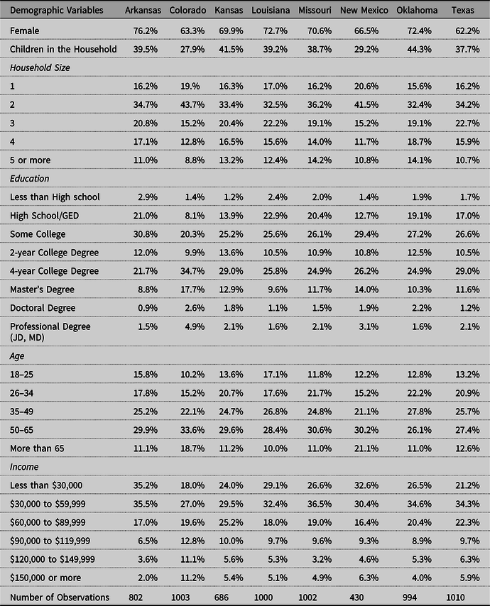
Although the survey was distributed to an eight-state region, the ultimate sample size for analysis reflected the individual state populations in terms of size and demographic representativeness. All respondents in the sample consumed milk at least once a week. The sample contains the following number of responses: 802 from Arkansas, 1,003 from Colorado, 686 from Kansas, 1,000 from Louisiana, 1,002 from Missouri, 430 from New Mexico, 994 from Oklahoma, and 1,010 from Texas. The survey data also included variables for demographics, location (county and state), choice decisions and questions designed to elicit ethnocentric (state pride) responses. For the purposes of this research, we also measured the shortest (haversine) distance from the geographic center of each respondent’s county to the individual state borders of the seven other states and included them in the dataset. The summary statistics for demographics by state are reported in Table 1.
Table 1. Summary Statistics of Demographic variables by State
To gauge the respondents’ preferences for different state labeled milk options, choice-based conjoint analysis was employed. Due to the ten possible labels (one for each of the eight states, regional, and national) and retail price per gallon ($2.75 or $4.50) a Partially Balanced Incomplete Block Design (PBIBD) was implemented. As a result, the survey included 20 choice sets. An example of the survey question can be seen in Figure 1. While survey fatigue is always a concern, the survey focused only on the choice questions with limited attributes and demographic information. As noted in the previous literature, there are tradeoffs in number of choice sets, choice alternatives, and additional questions (Chung et al., Reference Chung, Boyer and Han2011). In each choice question, respondents were asked to choose between four different gallons of milk, with the fifth option of not purchasing. While no food product is generalizable to all other products, milk has remained as a regional product even though most states have some level of milk production (Stephenson and Nicholson, Reference Stephenson and Nicholson2018). Thus, it is an interesting product to study within the context of substitution between regional and state branding programs.
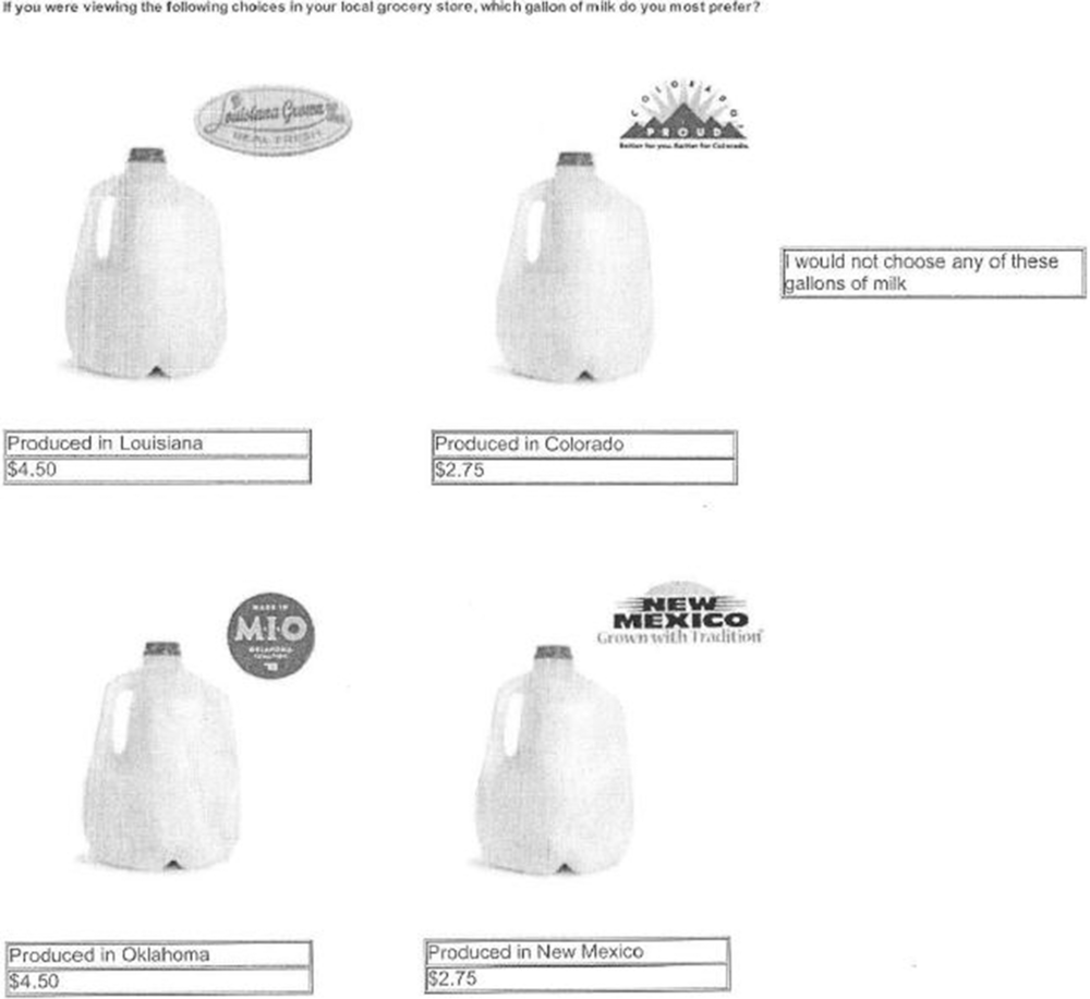
Figure 1. Example choice question used to determine respondent’s preference for state labeling.
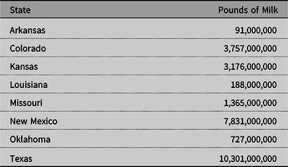
At the time of this survey (December 2015), the national average (median) retail price was approximately $2.84 ($2.81) per gallon, but milk prices had reached a national high within the previous 2 years of $4.01 per gallon and a low of $2.04 (USDA-AMS, 2015). Thus, the two prices used in the experiment ($2.75 and $4.25) represent prices below the mean/median and slightly above the highest price. Milk was chosen for this research as it is a fairly homogeneous product, in quality and packaging, as well as a staple food item for most households. Using a product with such generic attributes, more emphasis is placed on the labels, or prices, than on the specific product’s attributes. Within the region of interest, annual milk production varies from a high of 10.3 billion pounds of milk in Texas to a low of 91 million pounds in Arkansas (USDA-NASS 2015). Table 2 reports the production statistics by state.
Table 2. Milk Production by State in 2015 (Source: NASS, 2015)
3.1. Factor analysis and state pride
To elicit a state pride score, respondents were asked to rank on a five-point Likert scale, from strongly disagree to strongly agree, 12 statements from a version of Neuliep and McCroskey’s (Reference Neuliep and McCroskey1997) Revised GENE Scale that was modified to reflect consumer ethnocentrism at the state level. Half of these statements were worded positively toward the respondent’s current state of residence and the other half worded negatively.
To establish the level of state pride, factor demand analysis was conducted on the 12 pride statements and a flag value of 0.4 was used to ensure that each statement reflected its corresponding factor, as per Neuliep and McCroskey (Reference Neuliep and McCroskey1997). These factors were: (1) positive sentiments towards one’s state, and (2) negative sentiments toward one’s state. After removing statements that were double flagged and below the cutoff value, the factor analysis revealed ten questions (five positive and five negative statements) to be used in the state pride calculation. The statements were coded according to the question type: positive state sentiment questions were coded 1 (strongly disagree) to 5 (strongly agree) and negative state sentiment questions reverse coded. Through the summation of this coding, the respondent’s base pride score could range from a minimum of 10 to a maximum of 50. The ten statements used in the state pride calculation are included in Table 3.
Table 3. Adapted Statements from the Revised GENE scale for use in State Pride Calculation
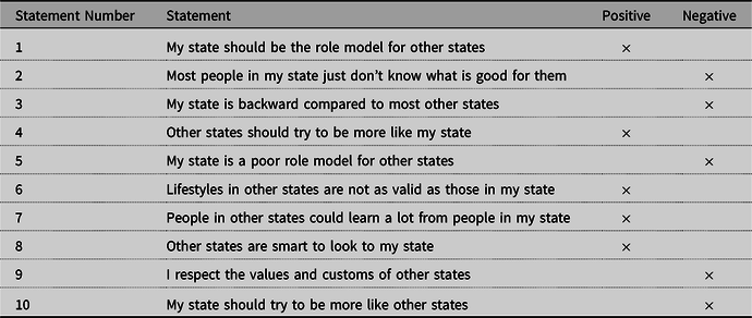
Note: Positive and Negative refers to the factor classes identified by Neuliep and McCroskey (Reference Neuliep and McCroskey1997).
4. Model
To determine the effects of the calculated state pride scores and distances, the data were analyzed on an aggregate (region) and disaggregate (state) level. A random parameters logitFootnote 1 model was employed to determine the heterogeneity of consumer preferences for both the regional and state-specific model. Derivations of own-state WTP from both models were estimated and compared to examine differences. Additionally, actual model comparisons via likelihood ratio were derived and used to determine overall model fit.
4.1. Regional model
The use of McFadden’s (Reference McFadden and Zarembka1973) Random Utility Model to estimate the consumer utility has become commonplace in examining discrete choice experiments. The typical utility model can be derived within a linear framework and is expressed as one state’s consumer choosing a labeled gallon of milk from the options across the region. While the regional model is an aggregated form of state-specific models, one is still able to estimate own- and cross-state WTP values since the individual states’ consumers are identified by distance and state pride scores. The pooled model is used to determine the effect of state pride scores and each consumer’s distance from neighboring state borders on preferences for state branded products on a regional scale. The general model is as follows:
 $${U_{ijn}} = {V_{ijn}} + {\varepsilon _{ijn}}$$
where ${U_{ijn}}$
is the utility that consumer, i, who resides in state, j, derives from choosing label, n, relative to the utility of choosing the “no milk” option;
${U_{ijn}}$
is the utility that consumer, i, who resides in state, j, derives from choosing label, n, relative to the utility of choosing the “no milk” option; ${V_{ijn}}$
is the observable or indirect utility from choosing label, j; and
${V_{ijn}}$
is the observable or indirect utility from choosing label, j; and ${\varepsilon _{ijn}}$
is the stochastic element of utility. The deterministic part of the utility equation, V, is constructed by
${\varepsilon _{ijn}}$
is the stochastic element of utility. The deterministic part of the utility equation, V, is constructed by
 $${V_{ijn}} = \;{\beta _i}{X_{ijn}} + \;\gamma Pric{e_n} + \mathop \sum \limits_{l = 1}^8 {\alpha _l}\left( {{X_{ij}}*{D_{ij}}} \right) + \mathop \sum \limits_{k = 1}^8 {\theta _k}({X_{ij}}*S{P_{ij}})$$
where β
i
is the individual-specific parameter for the corresponding attribute coefficients relative to the utility of the “choose no milk” option, and ${X_{ijn}}$
is a vector of attributes corresponding to state, region, or national labels. Label choices included dummy variables for Arkansas, Colorado, Kansas, Louisiana, Missouri, New Mexico, Oklahoma, Texas, Regional and National. Regional brand was represented by a private company, while national was represented by a national supermarket chain’s brand. Label preferences are assumed to be heterogeneous, denoted in a Random Parameters Logit model as
${X_{ijn}}$
is a vector of attributes corresponding to state, region, or national labels. Label choices included dummy variables for Arkansas, Colorado, Kansas, Louisiana, Missouri, New Mexico, Oklahoma, Texas, Regional and National. Regional brand was represented by a private company, while national was represented by a national supermarket chain’s brand. Label preferences are assumed to be heterogeneous, denoted in a Random Parameters Logit model as
 $${\beta _i} = \;\beta + {\eta _i}$$
where $\beta $
is the vector of mean label utility weights, and
$\beta $
is the vector of mean label utility weights, and ${\eta _i}$
is consumer i’s specific deviation from the respective mean (Zhang and Sohngen, Reference Zhang and Sohngen2018). Only the label alternative parameters are considered to be randomly distributed using a normal distribution.
${\eta _i}$
is consumer i’s specific deviation from the respective mean (Zhang and Sohngen, Reference Zhang and Sohngen2018). Only the label alternative parameters are considered to be randomly distributed using a normal distribution.
Price indicated the label price (either $2.75 or $4.50). ${D_j}$
represents the shortest distances from the geographic center of each respondent’s county to the j
th neighboring state’s border. For scaling purposes, the distances were divided by 10, while the respondent’s own state’s distance equaled zero. Distance was also recorded as zero for purposes of the regional and national labels. In order for distance to enter the model, it is interacted with the respective state label.
${D_j}$
represents the shortest distances from the geographic center of each respondent’s county to the j
th neighboring state’s border. For scaling purposes, the distances were divided by 10, while the respondent’s own state’s distance equaled zero. Distance was also recorded as zero for purposes of the regional and national labels. In order for distance to enter the model, it is interacted with the respective state label. $S{P_{ij}}$
represents the state pride score of the individual respondent (i) for his/her respective state (j). As with distance, state pride was interacted with each consumer’s own-state label.
$S{P_{ij}}$
represents the state pride score of the individual respondent (i) for his/her respective state (j). As with distance, state pride was interacted with each consumer’s own-state label.
4.2. State-specific model
To contrast the regional model an individual, state-specific model is used to represent disaggregated consumer preferences and heterogeneity. Similar to the regional model, the random variables were normally distributed and consisted of all 10 label options. The price, state distances and respective pride scores variables were all fixed. The model follows the same format as the regional model, except now there are 10 state-specific, s, models. Further, there is only one state pride parameter included. The state-specific indirect utility model is denoted as:
 $${V_{ijns}} = \;{\beta _{is}}{X_{ijns}} + \;{\gamma _s}Pric{e_{ns}} + \mathop \sum \nolimits_{l = 1}^8 {\alpha _{ln}}\left( {{X_{ijn}}*{D_{ijn}}} \right) + {\theta _s}({X_{ijs}}*S{P_{ijs}})$$
This model formula is similar to that presented in Neill, Holcomb, and Lusk (Reference Neill, Holcomb and Lusk2020), but these models now include distance and state pride parameters, which will lead to different estimates of WTP.
4.3. Marginal willingness to pay
Within this application, we focus on marginal WTP of the label alternatives and the effects of state pride and distance. As is standard in the literature, WTP is calculated as the negative ratio of the mean coefficient of interest and the price coefficient (Syrengelas et al., Reference Syrengelas, DeLong, Grebitus and Nayga2017). WTP standard errors are calculated via the Daly et al. (Reference Daly, Hess and deJong2012) method. Thus, a WTP value for a one-point increase in one’s respective state pride is calculated across the aggregate and disaggregate models. Accordingly, the regional model will estimate a state pride WTP value for each state; however, the state-specific models will only estimate state pride for that respective state. Similarly, for distance, the regional model will estimate WTP values for every distance measure while state-specific models will not have a WTP value for their own-state. We also estimate marginal WTP values at the average state pride scores for each state for comparison between the aggregate and disaggregate models. Finally, using Arkansas as an example, we present the marginal WTP distributions for state pride across all consumers between the two models. Using kernel densities of the distributions, one will be able to see the differences in distribution shapes.
4.4. Comparing aggregate and disaggregate models
It is likely that the aggregate and disaggregate models will lead to mixed WTP measures that do not present a clear distinction on model fit. Thus, we derive a joint Likelihood Ratio (LR) test for equality between the aggregate and disaggregate models. Using the Log-Likelihood (LL) from each model:
 $$LR = 2*\left( {L{L_{region}} - \mathop \sum \limits_{s = 1}^S L{L_s}} \right)\~\ \chi _{{m_s}*s - {m_{region}}}^2$$
where $L{L_{region}}$
and
$L{L_{region}}$
and $L{L_s}$
are the regional (aggregate) and state-specific (disaggregate) model log-likelihood values. The LR test is distributed chi-squared and has degrees of freedom equal to the number of parameters across all state-specific models,
$L{L_s}$
are the regional (aggregate) and state-specific (disaggregate) model log-likelihood values. The LR test is distributed chi-squared and has degrees of freedom equal to the number of parameters across all state-specific models, ${m_s}*s$
, minus the number of parameters in the region model,
${m_s}*s$
, minus the number of parameters in the region model, ${m_{region}}$
. Specifically, the degrees of freedom in this case is 121, since
${m_{region}}$
. Specifically, the degrees of freedom in this case is 121, since ${m_s}$
= 19, s = 8, and
${m_s}$
= 19, s = 8, and ${m_{region}}$
= 31.
${m_{region}}$
= 31.
5. Results
The results of the RPL model suggest significant heterogeneity within the regional and state-specific models for own and cross state labels (Table 4). Within the regional model, consumers have the strongest average preference for the Regional label. As expected, consumer pride scores have a positive impact on own state preferences and distance has a negative effect on cross state preferences. Once the data is disaggregated, the state-specific models reveal that consumers may have stronger preferences for the regional or national labels rather than their own state label. One surprising result from the Oklahoma state model is that the pride score has a negative and statistically significant impact on utility. All other fixed coefficients that are statistically significant have the expected signs.
Table 4. Random Parameter Logit Estimates for the Regional and State-Specific Models
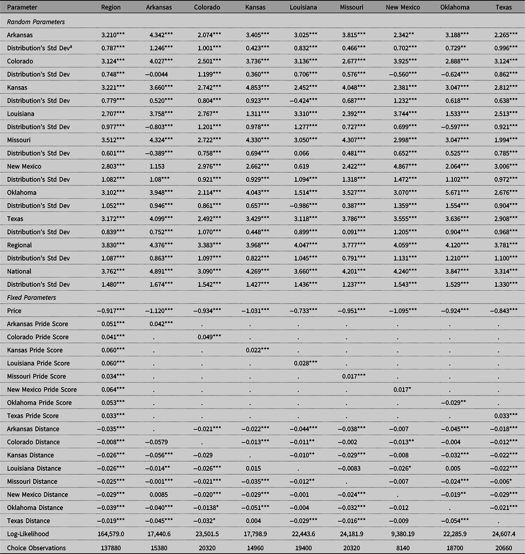
Note: *, **, *** denote statistical significance at the 0.10, 0.05 and 0.01 levels, respectively (Standard errors are removed for readability).
a Estimates are standard deviations of the alternative specific constants.
5.1. Willingness to pay between aggregate and disaggregate data
To ease the interpretation of the results, Table 5 presents the marginal WTP values for each of the attributes, including interaction terms (state pride and distance). On an aggregate (regional) level, consumers are willing to pay the most for the regional label on average, $4.18, followed by the national label, $4.10. For the state labels, consumers across the whole region have the highest marginal WTP for the Missouri label ($3.83) and the lowest WTP for the Louisiana label ($2.95). Kansas, Louisiana, and New Mexico consumers have the highest marginal WTP for one-point increases in state pride scores, with Colorado and Texas consumers having the smallest marginal WTP. This may be an example of diminishing marginal WTP for a one-point change in pride scores, as Colorado and Texas consumers have the highest average state pride scores. When considering out-of-state consumers, marginal WTP discounts for distances vary between $0.01 and $0.04 per 10 miles. Within the sample some consumers live more than 800 miles from certain state borders, which could impact marginal WTP by more than $3.20.
Table 5. Regional and State-Specific Model Estimates of Own and Cross State Marginal Willingness-to-Pay Estimates
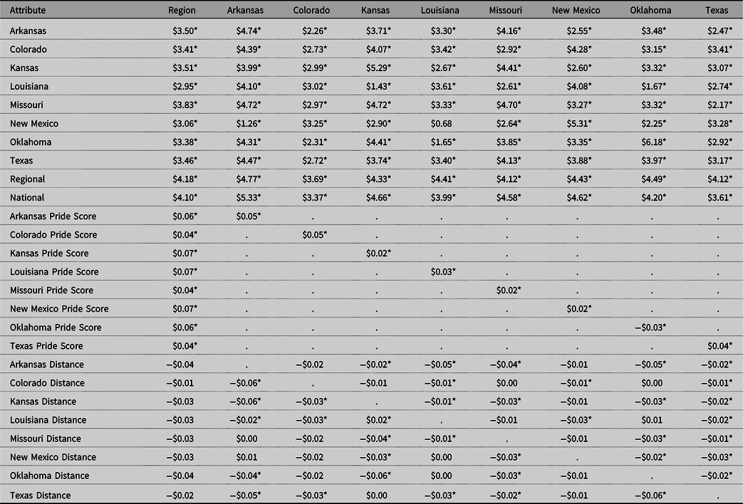
Note: * denotes statistical significance at the 0.05 level (Standard errors are removed for readability, but available upon request).
When looking across the disaggregate models (state-specific), only Kansas, Missouri, New Mexico, and Oklahoma consumers have a higher marginal WTP for their own state label as compared to all other labels. Colorado, Louisiana, and Texas consumers have the highest marginal WTP for the regional label, while Arkansas has the highest marginal WTP for the national label. Excluding Arkansas and Texas, the marginal WTP of state pride for each state’s consumers is less than the WTP from the regional model. Again, Oklahoma consumers experience a negative marginal WTP from increases in state pride, which contradicts the expected result. These results are quite different from that of Neill et al. (Reference Neill, Holcomb and Lusk2020) as they found that all states, except Texas and Louisiana, have the highest WTP for their own brand. Our results suggest much more heterogeneous preferences when distance and state pride are accounted for within the model. As for distance from the state specific models, almost all have the expected negative sign or are zero. The effect of distance is heterogeneous across the disaggregate models, which is expected as distances to different states are relative due to the geographical position.
Although Oklahoma has a negative and significant coefficient for the pride score, it also has the highest marginal WTP for the state logo ($6.18). Furthermore, New Mexico has the lowest average pride score, but one of the highest marginal WTP for the local label ($5.31). Last, Texas has a high average pride score, but a low marginal WTP. To the detriment of state marketing programs, this result could indicate that state pride does not play as significant a role in consumers’ WTP.
5.2. Comparing aggregate and disaggregate models
While it is easy to interpret the marginal WTP for state pride from model estimates, the more interesting WTP measure is the marginal WTP at the average state pride score for each state. Figure 2 presents the distribution of WTP from the aggregate and disaggregate models. Colorado consumers had the highest average state pride score at 34 out of 50, while New Mexico consumers has the lowest score at 27 out of 50. Only 0.3% of all consumers in the sample fell at one of the extremes (10 or 50) and the overall average pride score was 30. Upon examination of the differences, the aggregate model almost always estimates a higher average WTP than the disaggregate models. The average difference over the state-specific models, excluding Colorado and Texas, is $1.18 at the average state pride score.

Figure 2. Histograms and kernel densities of marginal WTP for all state pride scores between the regional and state-specific model.
From the marginal WTP related to the state pride values, the regional model overestimates WTP for some states and underestimates for other states in comparison to the state-specific models. This supports the hypothesis of masked heterogeneity from aggregated models. To demonstrate the aggregate and disaggregate models’ differences, we calculate marginal WTP for each consumer based on individual state pride scores. The distributions and resulting kernels for all states are shown in Figure 2. Using Arkansas as an example, it is clear from kernel mapping that the regional marginal WTP distribution has a higher mean ($1.75 vs $1.46). The kernel also reveals some differences in variance. Using an F-test for equal variances, we find that there is a statistically significant difference at the 5% level between the variances of the two distributions (F = 1.44 with 754 degrees of freedom)Footnote 2 . Next, we perform a formal LR test as presented in equation (7). The chi-squared value between the aggregate and disaggregate models is equal to 5,878.02 which is significant at the 1% level. Between the visual examination and the formal hypothesis tests, we find that aggregate and disaggregate models will lead to non-negligible differences in marginal WTP distributions.
6. Discussion and conclusions
State branding programs for agricultural products were designed to promote in-state agricultural sustainability and increase regional economies (Govindasamy et al., Reference Govindasamy, Italia and Thatch2000). The intentions of state brands are to leverage public funds to generate net economic gains for states’ agricultural industries, yet previous studies suggest that the predominant marketing strategy of merely adding a state brand to a product label may not generate the desired consumer response (e.g. Collart et al., Reference Collart, Palma and Carpio2013). Studies such as Khachatryan et al. (Reference Khachatryan, Rihn, Campbell, Behe and Hall2018) suggest that a lack of understanding regarding consumers’ perceptions of “local” can lead to conflicting results when assessing perceptions across a large population base. These imperfect, and sometimes conflicting, consumer preference results may be due to the exclusion of other factors, such as consumer loyalty to a regional brand or proximity to neighboring states with similarly valued, state-branded products.
This study provides a unique but replicable assessment of the values consumers place on products from their own states and neighboring states, including the impacts of state pride, border proximity, and the presence of recognized regional and national brands on WTP calculations. For economists analyzing the impacts of state market promotion programs, this study may provide insights on more inclusive explanatory variables for assessing the values associated with brands. Specifically, incorporating beliefs (state pride) and geographic information (distances) significantly changes the results and corresponding WTP estimates.
Because state marketing programs constitute public dollars being spent on advertising and promotion efforts for private goods, the spill-over effects for state-labeled products marketed across state lines should be considered. As Hinrichs (Reference Hinrichs2003) notes, state officials may tout the existence of state-based promotional efforts without fully recognizing or understanding that a spatially defined marketing effort needs to consider social and environmental relations that may also be spatialized within/near the state’s borders. Recognizing the heterogeneity of consumer attitudes towards a state brand, even within the state, may help state program administrators better target the use of public funds towards more impactful marketing campaigns.
The findings from this study are consistent with the arguments of Hand and Clancy (Reference Hand, Clancy, King, Hand and Gomez2014), Collart et al. (Reference Collart, Palma and Carpio2013), and Khachatryan et al. (Reference Khachatryan, Rihn, Campbell, Behe and Hall2018), suggesting that evaluations of consumers’ preferences for state labeled products needed to be more robust to obtain accurate measures of program impact. Comparing our results to that of Neill et al. (Reference Neill, Holcomb and Lusk2020), we find that consumers do not necessarily have the highest preference for their own state’s products. As shown, three of the state-specific models and the regional model suggest that the Regional label has the highest preference for milk among consumers. This supports previous work suggesting that a collective action to advertising may result in higher welfare (Alston et al., Reference Alston, Freebairn and James2001; Crespi and James, Reference Crespi and James2007; Cakir and Balagatas, Reference Cakir and Balagtas2010). General commodity advertising programs, and corresponding producer check-off programs, likely also affect the consumer views on milk, which are not discussed in this study since the focus was specifically on state branding programs.
The results are not homogenous between the regional and state-specific models and show a tradeoff in model estimates between raw preferences for state labels and the effect of state pride. Thus, the answer to our question about a consumer’s proximity to state borders and the level of state pride affecting WTP for different brands is mixed. Some states’ consumers are more sensitive to measures of state pride than other states. Distance shows to have a negative effect, if any effect at all, on WTP. These types of issues would not be as relevant in generic commodity advertising.
While this work has contributed to the literature on state and regional branding programs, there are several limitations worth noting. First, this study does not include other consumer beliefs about local and regional food such as environmental, health, and local economy benefits. Previous studies have shown that these beliefs can vary greatly across a sample population, including consumers’ personal definitions of “local” or “healthier” (e.g. Holcomb et al., Reference Holcomb, Neill, Lelekacs, Velandia, Woods, Goodwin and Rainey2018; Khachatryan et al., Reference Khachatryan, Rihn, Campbell, Behe and Hall2018; Hand and Clancy, Reference Hand, Clancy, King, Hand and Gomez2014), yet they can play a role in WTP for state branded products. Second, our study is limited to one homogeneous product which does limit the generalizability of the results to all other types of products. Finally, our study does not look at the tradeoffs between geographical production labels and other attributes of milk. While the last limitation would be of interest, it may also confound the results and should be carefully approached in future research.
This study also contributes to the growing literature on the masking of consumer heterogeneity within pooled/aggregated models (e.g., Lusk, Reference Lusk2017; Malone and Lusk, Reference Malone and Lusk2017; Neill and Holcomb, Reference Neill and Holcomb2019). Like other recent studies, the findings illustrate the importance of considering the degree of consumer heterogeneity present within samples when comparing aggregate versus disaggregate models. From the marginal WTP values for state pride and formal tests of equality, we have demonstrated that there are non-negligible differences between aggregate and disaggregate models. Policy makers need to be keenly aware that aggregated models may overestimate the impacts of a marketing program on consumers’ preferences and WTP, meaning less “bang for the buck” from tax-payer-funded promotional programs.
Acknowledgements
The authors would like to extend our appreciation to Jayson Lusk for his advice and suggestions on survey design and discussions about the general research topic. Financial support is provided by the Oklahoma Agricultural Experiment Station and the Browning Endowed Professorship Fund.


 Open access