


1. Introduction
In the course of the trend toward the intelligent factory as part of the future project Industry 4.0, manufacturing companies are faced with considerable tasks. Sales markets demand greater flexibility, products must be customizable and, at the same time, products and their manufacturing processes are becoming more complex. Depending on the intended use, these should be able to process a large number of different components and raw materials in small quantities at the same time. Increasing complexity of the process sequences is accompanied by increasing demands on automation. This in turn is supported, facilitated, or made possible in the first place by a broad, reliable, and immediately available information base.
In order to achieve a consistently high production quality even with small consumption quantities and dynamic processes, all relevant control variables of an automated manufacturing process must be permanently available. These include the filling quantities of liquids, viscous substances, and free-flowing bulk materials in an increasing number of small and application-specific geometrically adapted storage and process containers, which must be continuously recorded by sensors, as shown in Fig. 1. These level measurements are realized with a wide variety of measuring methods, all of those have their advantages and disadvantages. Optical sensors, for example, have potentially high accuracy. However, they reach their limits, in case of adverse visibility conditions.

Fig. 1. Example of a modern factory, where fill level measurements play an important role.
Contact-based measurements, such as guided wave radars [Reference Wegner, Del Galdo and Gebhardt1, Reference Kaineder, Stelzer, Michenthaler and Hammerschmidt2] or capacitive probes [Reference Kumar, Rajita and Mandal3, Reference Chetpattananondh, Tapoanoi, Phukpattaranont and Jindapetch4], have the major disadvantage that they are not suitable for volumetric measurement of a complete container, since, depending on the application, bulk cones can also form. Contactless radar measurements have the advantage that they can measure volumetrically. The disadvantage is the large number of multipath propagation components, especially in closed metal containers, which can negatively influence the measurement. To reduce this effect, electrically large [Reference Vogt and Gerding5, Reference Heddallikar, Rathod and Pethkar6] or lens antennas [Reference Vogt7] are often used to focus the beam of the electromagnetic waves. In small containers, however, this is not practical, since the installation space does not allow for large antennas. In addition, this means that volumetric measurement is only possible to a limited extent. For this reason, this paper investigates the feasibility and achievable accuracy of volumetric radar level measurement with an electrically small patch antenna under the influence of large multipath components.
In a first step, the accuracy of an M-sequence ultra-wideband (UWB)-guided wave radar is analyzed and it is investigated whether it is suitable as a reference system for other level measurement systems. The main advantage of a guided wave radar is the elementary propagation of the electromagnetic wave. In fact, as the wave is guided along a line or cable, no multipath propagation occurs. This allows a very high accuracy to be achieved. After successful evaluation of the guided wave radar as a suitable reference system, the results of the contactless level measurement are shown and discussed.
2. Background
In this paper, results of contact-based measurements using a guided wave radar as well as results of contactless radar measurements are shown. For reasons of simplification, the signal processing in this section is described using the guided wave radar. The algorithms used can also be adapted to the contactless measurements with slight additions. These additions are explained in the corresponding section of the result analysis.
The main principle of a guided wave radar is based on a time-domain reflectometer [Reference Cataldo, Tarricone, Vallone, Attivissimo and Trotta8]. The electromagnetic wave emitted by a radar travels along a wire. When this wave encounters a medium transition, such as water surface, part of it is reflected and another part penetrates the medium. The reflected signal is received again and the level can be determined by measuring the time of flight, analogous to distance determination in radar technology. This principle is shown in Fig. 2. On the left there is the resulting signal with the reflection of the wire connection or feeding point, because it is not perfectly matched, the reflection of the water surface, the reflection of the bottom as well as some multiple reflections at the container wall.

Fig. 2. Resulting signal reflections of a guided wave UWB radar inside a container and illustration of the principle of level measurement.
2.1 Delay time estimation
If one wants to analyze the accuracy of the level measurement, the calculation of the distance or delay time must be considered more closely. A physically realizable signal always has a temporal extension, which depends in particular on the bandwidth. Accordingly, there exist the most different definitions for the time position of an impulse, for example by exceeding a threshold value, the maximum of the impulse, or the energetic center [Reference Sachs9]. For the analysis in this work, the temporal position of a selected pulse maximum was used, since this yielded the best accuracy in preliminary studies. In order to be able to specify a precise assignment of pulse maximum and filling level, a calibration measurement is necessary.
To achieve an accuracy of the delay estimation below the sampling interval $\Delta t$ , the data are usually first interpolated. The fast Fourier transform method using zero padding in the frequency domain is suitable for this. Additionally, a fourth-order polynomial adjustment is performed around the searched maximum of the interpolated received signal, and then the position of the zero crossing (sign change) of the first derivative is searched for. With this method, given the high signal to noise ratio by measuring with a guided wave radar, a time resolution of $10^{-4}\Delta t$
 could be achieved. This corresponds to an accuracy of some micrometers, which is directly dependent on the clock frequency [Reference Sachs10].
A consistent high accuracy of the level measurement over the complete container height has, however, further prerequisites. The signal shape must not change over the observation time and fill height. Only if the signals to be compared have an identical shape can two identical states (e.g. maxima) be compared with each other. If the shape of the pulse changes even minimally, the position of the maximum used for estimating the time delay also changes. The consequence is a falsification of the level measurement. One reason for the signal deformation can be interference with other static or quasi-static reflections also known as background, e.g. by mismatch of the feeding point. For this reason, these interfering reflections must be subtracted from the intended signal.
2.2 Background subtraction
In order to subtract quasi-static background components, e.g. due to temperature drift effects, the background must be continuously recalculated. A real-time capable background subtraction (BS) method is given by an exponential averaging [Reference Zetik, Crabbe, Krajnak, Peyerl, Sachs and Thomä11]. We estimate the background $\bar {h}$ for each observation time indexed by $k$
 with
with

where $\bar {h}_k$ and $\bar {h}_{k-1}$
 are the estimated backgrounds for time indices $k$
 and $k-1$
 , $h_{k}$
 is the impulse response, $\alpha \in [ 0,\; 1]$
 is a scalar weighting factor, and $\beta$
 is a binary value which is based on the calculated difference between two consecutive impulse responses. The optimal value for $\alpha$
 was experimentally determined to be $\alpha = 0.99$
 for both contact-based and contactless measurements. As initial background, we use the measurement of the empty container, where the reflection of the bottom and subsequent multiple reflections are set to zero. Therefore, these reflections are not part of the initial background. The resulting signal $\hat {h}_k$
 is now

A special case arises if the fill level does almost not change a moment. In this case, $\bar {h}_k$ approaches $h_{k}$
 with (1) and $\hat {h}_k$
 only consists of noise if $\beta$
 is not introduced. Therefore, we set $\beta$
 according to the calculated intensity of level change $\gamma _k$
 inspired by [Reference Lee, Choi and Cho12]

We set $\beta _k = 1$ if $\gamma _k$
 is above a certain threshold and $\beta _k = 0$
 otherwise. In the latter case, no update of the background is performed. To minimize the influence of the slow occurring temperature drift, the current temperature at the antenna is compared in parallel with the temperature at the time of the last update of the BS, if $\beta _k = 0$
 . If the temperature difference near the feeding point exceeds 0.1 K, $\beta _k = 1$
 is set for one measurement to be able to compensate very slow temperature drift effects even at long lasting level.
3. Measurement setup
To analyze the accuracy of the level measurement and the long-term stability, it is essential to be able to carry out reproducible measurements and to approach the levels under investigation with sufficient accuracy. Great importance was attached to these two aspects when designing the experimental measurement setup. The actual measurement setup is shown in Fig. 3 and as a detailed sketch in Fig. 4. The reference measurement and the test measurement are carried out in two separate containers so that the systems do not influence each other. Both containers are connected via a pipe and are always filled or emptied simultaneously via a water reservoir.

Fig. 3. Experimental setup for the evaluation of liquid level measurements by an M-sequence UWB-guided wave radar.
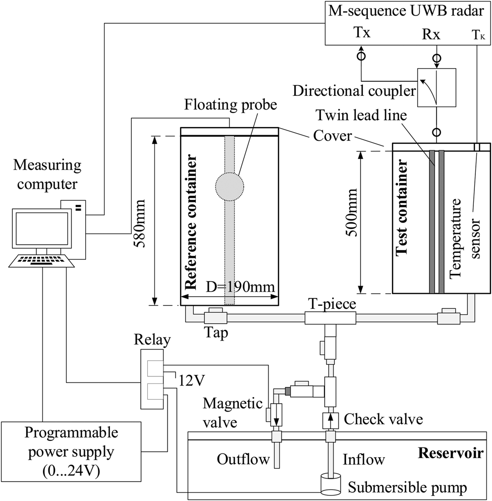
Fig. 4. Experimental setup for the evaluation of liquid level measurements by an M-sequence UWB-guided wave radar.
The principle is used that the level in two connected containers balances each other out. This principle reaches its limits during dynamic processes like filling and emptying. The dynamic balancing processes between the containers must be taken into account. In order to balance the levels in the containers, a level must be maintained for a certain period of time. This will be discussed in more detail in the next section.
A floating probe with an accuracy of 0.5 mm over the entire height of the container is located in the reference container. The test container contains a twin lead cable, which is fed via an $12{\rm th}$ -order M-sequence radar with a clock frequency of 13.3 GHz featuring 6 GHz bandwidth supplied by Ilmsens GmbH. An M-sequence has various advantages compared to pulse signals such as low crest factor and a high time stability. To get the raw impulse response of the scenario for further analysis, a wideband correlation between transmit and receive signals is performed. A more detailed description of the principle can be found in [Reference Sachs, Peyerl and Roßberg13].
This is a high-priced radar for experimental setups. However, it can be integrated and would therefore be cheap for large quantities.
For automation purposes, a solenoid valve and a water pump are connected to a relay which is controlled by the measuring computer. To be able to additionally vary the speed of the water supply, a programmable laboratory power supply was used. The ability to accurately approach the level allows a much more accurate analysis than in [Reference Pečovský, Galajda, Sokol and Kmec14], where the level change was only simulated by moving the complete container using a positioner.
4. Contact-based measurement
In this section, the accuracy of a guided wave radar will be analyzed. The aim is to investigate whether a guided wave radar is comparable with commercially available reference systems and can therefore act as a reference system itself.
A large number of measurements were carried out to analyze the accuracy of the level measurement. As an example, water is used here as the filling material, as many industrial products contain a large percentage of water. Other fluids such as liquid glue and oil were also tested, showing similar accuracy.
4.1 Measurement data
In Section 2.1 it was mentioned that a constant pulse shape is essential to achieve high accuracy in level measurement. Any deformation of the pulse due to, e.g. interference would affect the accuracy. These interference effects can be seen, e.g. in Fig. 5. This is a measurement in which the container is filled continuously at the beginning until the container is completely full. Then the container is emptied step by step by 1 mm until the container is completely empty. Each fill level was held for approximately 1 min to allow the levels in the reference container and test container to equalize. Due to the very small step size, the stepwise measurement is not visually visible in the data. However, this explains the measurement duration of approximately 610 min. The stepwise measurement and its effects will be discussed in more detail in the next section. At high filling levels, the reflection of the medium overlaps with the reflection of the feeding points. For reasons of better visualization, only a section of the measurement data is shown. The actual length of the impulse response is about 300 ns.

Fig. 5. Radargram of a container being emptied recorded by a contact-based M-sequence UWB-guided wave radar before BS.
The resulting signal after BS is shown in Fig. 6, where the influences of interference were minimized. The reflection of the water surface and the container bottom is clearly visible. The reflection caused by the bottom has a different slope because the propagation speed in water is lower than in air.

Fig. 6. Radargram of a container being emptied recorded by a contact-based M-sequence UWB-guided wave radar after BS.
The results show that BS is indispensable, otherwise static reflections, such as those of the feeding point, would significantly worsen the accuracy of the measurement.
4.2 Fill level measurement
As mentioned above, the measurement system has dynamic effects that must be taken into account in the analysis. For this reason, the container was emptied step by step. To illustrate this, the measured level in the reference container and in the test container during emptying is shown in Fig. 7.

Fig. 7. Comparison of two measuring systems with regard to the reaction time of level changes and measuring accuracy.
First, the container is emptied, the solenoid valve closes and the levels in the containers equalize. The maximum duration of the equalization process was 30 s. The measured values of the equalized level were used for the analysis. On the right, it can be seen how the measurement systems react when the solenoid valve opens. The measurement in the test container (UWB system) reacts faster than in the reference container. In particular, we can see two effects that overlap, the dynamics of the overall system (two connected containers) and the different dynamics of the measuring instruments. An exact separation of these effects is not possible on the basis of this measurement. This will be discussed in more detail in the section on contactless measurement.
For the analysis of the system we distinguish between accuracy and precision. The accuracy describes the difference between the reference level and the measured level over all levels.
The results of the accuracy analysis are shown in Fig. 8. The graph shows the maximum difference between the reference and test measurement for each level approached. An accuracy of better than 0.5 mm could be achieved up to a fill level of 2 cm below container top. An accuracy of at least 0.9 mm could be demonstrated for the last 2 cm. One of the reasons for the lower accuracy is that there are strong interference effects with the feeding point, which could not be completely eliminated even by BS.

Fig. 8. Accuracy of the M-sequence UWB-guided wave radar in comparison with a floating probe. A 0.5 mm accuracy in the green area, 0.9 mm in the orange area.
It should be noted that the reference system used here is specified with an accuracy of 0.5 mm. An exact analysis of the accuracy is therefore limited to this 0.5 mm. The precision describes the maximum distance between mean value and measured value of a level. To determine the precision of the measuring system, the mean value of each level approached was calculated and the maximum distance was determined. The precision of the system is found by taking the maximum of the value over all levels. The precision of the reference system is 31 ${\rm \mu }$ m. With 3 ${\rm \mu }$
 m the precision of the UWB system is more than 10 times higher under laboratory conditions. In addition, the floating probe reacts to level changes with a delay. This is probably due to the mass inertia of the probe and static friction effects between guide rail and float. Both effects do not occur with UWB measurements. The UWB system can thus measure the level with better accuracy and precision compared to a currently commercially available reference system. This makes this system suitable as a reference system for other sensors.
5. Contactless measurements
In this section, the achievable accuracy of volumetric radar level measurement with an electrically small patch antenna, also fed with a 12th-order M-sequence UWB radar, is investigated under the influence of large multipath components, see Fig. 9. For the analysis in this paper, a closed metal container was chosen, since the multipath propagation that occurs strongly here represents a major challenge in level measurement.

Fig. 9. Experimental setup for the evaluation of contactless liquid level measurements by an M-Sequence UWB radar.
In the previous section, it was shown that the guided wave radar under investigation can be used as a reference measurement for contactless radar measurement. The choice of the UWB-guided wave radar as a reference system has the additional advantage that the measured values of the reference system and the test system can be easily synchronized in time. For the contactless measurements, the guided wave radar is therefore taken as the reference.
5.1 Measurement data
To better illustrate the differences between contact-based and contactless measurements, a similar measurement was used to illustrate the results in this paper. This measurement is shown in Figs. 10 and 11 before and after BS. Compared to the measurement data of the contact-based measurement as shown in Fig. 5, a significantly higher influence of multipath components and interference due to the antenna feeding point can be seen. The interference due to the antenna feeding point can be eliminated to a major degree by BS, see Fig. 11. A closer look at Fig. 11 reveals a large number of multipath components. In addition, the pulse shape is strongly deformed at very high levels just before the antenna. This affects the accuracy, as described in the next section.

Fig. 10. Radargram of a container being emptied recorded by an M-sequence UWB radar before BS.
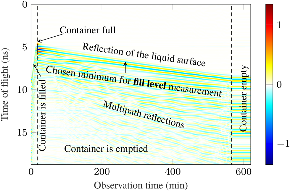
Fig. 11. Radargram of a container being emptied recorded by an M-sequence UWB radar after BS.
In the case of guided wave radar, there was a clear maximum that was suitable for level measurement. With contactless measurement, this is not the case due to the high number of multipath components. With contactless measurement, there are a large number of maxima and minima that can be used. However, looking at the radargram in Fig. 11, there is exactly one minimum that has sufficient amplitude and is only slightly affected by multipath components. For this reason, this minimum was used for the level measurement. This is the first minimum which exceeds a threshold value of 50 % of the corresponding global pulse minimum. By choosing such a threshold, no further tracking algorithm is needed.
5.2 Contactless fill level measurement
For the analysis of the measurements, attention was paid to the fact that the algorithm can also be used in practical, industrial applications. For this reason, an empty level calibration was performed for the analysis of the measurements, and thus the zero level was defined. An increased accuracy can be achieved, e.g. by a 3-point calibration.
The results of the accuracy analysis are shown in Fig. 12. An accuracy of better than 3 mm could be achieved up to a fill level of 2 cm below container top. An accuracy of at least 16.7 mm could be demonstrated for the last 2 cm. The main reason for the low accuracy in the last 2 cm is the pulse deformation due to the measurement in the near field of the antenna. For practical applications the accuracy in the near field of the antenna would be too low. Furthermore, it was checked whether the course of the curve, which can be seen in Fig. 12, can be assumed to be partly systematic. For this purpose, the accuracy values for each level were stored in a table in 1 mm steps (look-up table). The current measured level was then corrected by the value of the nearest neighbor in the table. Taking into account the curve progression or the calibration table, an accuracy of 0.6 mm could be achieved. However, such a calibration measurement is not practical in many applications. For this reason, it will be shown in the next section how to define the full state more precisely.
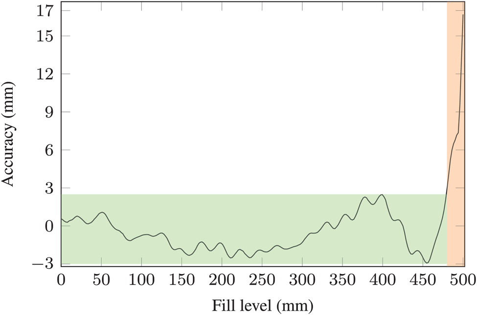
Fig. 12. Accuracy of the contactless M-sequence UWB radar compared to the guided wave radar evaluated above. A 3 mm accuracy in the green area, 16.7 mm in the orange area.
Figure 13 shows a similar representation as Fig. 7. A big difference can be seen at the bottom right. In Fig. 13, the reference system and the test system (both UWB systems), detect the emptying simultaneously. In Fig. 7 a delay of the reference system can be seen. This behavior could be observed over all filling levels. Furthermore, a more continuous course of the level change in the reference container during the equalization process is visible. Thus, it can be assumed that both contact-based and contactless level measurement can be performed more dynamically by using an M-Sequence radar than with the commercially available reference system described in Section 3. One reason for the delayed response time of the floating probe may be that the probe slides along a rail. This causes friction effects to occur. These frictional effects can also explain why a more continuous change of the level during the balancing process of the two containers can be seen here than in Fig. 7.
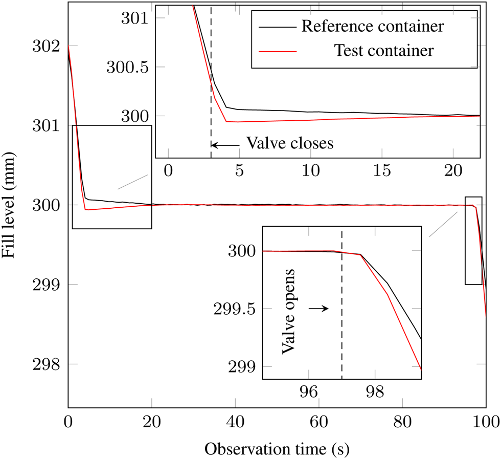
Fig. 13. Comparison of the reference (guided wave radar) and the test system (contactless radar) with regard to the reaction time of level changes and measuring accuracy.
The precision was defined in Section 4.2 and also determined for this system as the maximum value over all levels. A precision of 30 ${\rm \mu }$ m could be achieved under laboratory conditions.
5.3 Full state measurement
Depending on the application, the accuracy of the level measurement mentioned above may not be sufficient, especially for limit levels. Thus, the overflow of a container should be prevented in any case. For this reason, it is of great interest to be able to accurately detect the full state of a container. In the case of the container used, the full level is reached at an exact filling level of 500 mm.
With level determination based on time-of-flight or distance measurement, pulse deformation leads to a loss of accuracy, as already mentioned several times. This pulse deformation is now to be exploited for full state measurement, since the signal changes significantly here. To illustrate this, a section of the impulse responses for different levels up to full state is shown in Fig. 14. In addition to the change in shape, a clear increase in amplitude can also be seen.
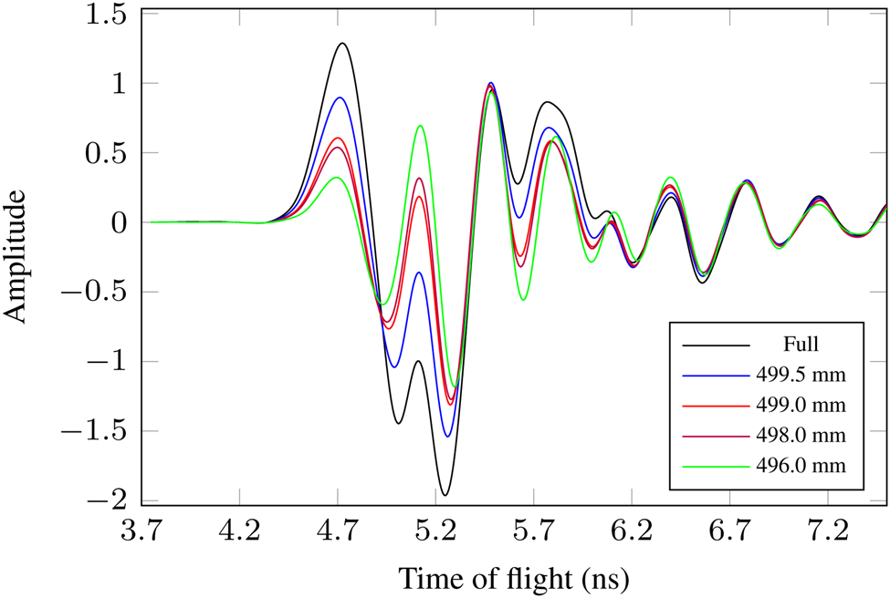
Fig. 14. Pulse deformation at full state of the container illustrated over several filling levels.
As mentioned above, an empty level calibration is made for the level calculation. In order to have the most practical solution for the full state determination, no further full state calibration was made, but the existing empty level calibration measurement was used. For the estimation of the full limit state, the impulse response of this calibration measurement $\bar {h}_E( t)$ is stored and subtracted from the currently measured impulse response $h_{k}( t)$
 and the mean squared error $MSE_k$
 compared to the empty state is calculated

The course should be as follows. When the container is empty, $MSE_k$ approaches zero. At medium levels, the curve should be almost constant, since the amplitude ratios in the signal do not change. As soon as the level is close to the antenna, $MSE_k$
 should increase, because especially increasing amplitudes can be detected. The results of this method are exemplified in Fig. 15. At medium levels, the $MSE_k$
 is at an approximately constant level. As soon as the container becomes empty, the $MSE_k$
 goes almost to zero. As the level approaches the full state and thus the near field of the antenna, the $MSE_k$
 increases rapidly. This rapid increase can be used to define the full state, e.g. by exceeding a threshold value. The investigations have shown that the impulse response of the empty container is time-stable. Thus, it was possible to define a time-stable threshold for $MSE_k$
 of 200 above which the container is assumed to be full.
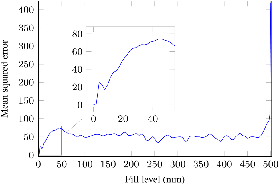
Fig. 15. Results of the full limit state measurement of water in a closed metal container
The measurement was repeated several times over the course of a year to test the long-term stability of the system. An accuracy of 0.5 mm could be achieved for the full state indication, whereby the threshold value was not changed. The calibration measurement of the first measurement run was used for the analysis. Thus, it could be shown that the calibration is also stable in the long term. This is particularly interesting for practical applications.
6. Conclusion
In this paper, contact-based and contactless level measurement in small metallic and non-metallic containers using an M-sequence UWB radar featuring 6 GHz bandwidth were presented.
In contact-based measurements using a guided wave radar, levels could be measured in the sub-millimeter range. It was shown to provide more precise and dynamic measurements than a commercially available reference system. A precision of 3 ${\rm \mu }$ m was achieved in the detection of fill level fluctuations. This enables the detection of the smallest fluctuations in the level of liquid materials and could play a major role in the future, e.g. in machine operation or diagnostics.
In contactless volumetric level measurements, it was shown how a simple empty level calibration could be used to achieve an accuracy of better than 3 mm up to close to full state. A precision of 30 ${\rm \mu }$ m could be achieved in the detection of level fluctuations. In addition, it was shown how to carry out a sub-millimeter accurate full state measurement independently of the actual level measurement. This allows accurate level measurement over the complete container height without dead zone.
In this paper, level measurements were carried out in cylindrical vessels. The influence of the container height and diameter is currently under investigation. Next steps could be to investigate more complex container geometries. In fact, in many applications containers have tubings and other internals which will influence the measurement, making their investigation of great interest for industrial applications.
Acknowledgments
This work was partly supported by the German Federal Ministry for Economic Affairs and Technology (BMWi) under research contracts ZF4463501RR7 and ZF4087105RR7.
 Tim Erich Wegner received his B.Sc. and M.Sc. degrees in electrical engineering and information technology from Technische Universitét Ilmenau, Germany, in 2016 and 2018, respectively. He is a researcher at the Electronic Measurement and Signal Processing Group and pursuing his Dr.-Ing. degree. His research interests include signal processing and data fusion for ultra-wideband radar applications.
 Stefan Gebhardt studied industrial and electrical engineering at Technische Universitét Ilmenau. In 2014, he received his doctoral degree in the topic of capacitive tomography. He is currently working as a senior development engineer at RECHNER Sensors GmbH, where he is responsible for research activities and developments in the field of level measurement technology.
 Giovanni Del Galdo studied telecommunications engineering at Politecnico di Milano. In 2007, he received his doctoral degree from Technische Universitét Ilmenau on the topic of MIMO channel modeling for mobile communications. He then joined Fraunhofer Institute for Integrated Circuits IIS working on audio watermarking and parametric representations of spatial sound. Since 2012, he leads a joint research group composed of a department at Fraunhofer IIS and, as a full professor, a chair at TU Ilmenau in the research area of electronic measurements and signal processing. His current research interests include the analysis, modeling, and manipulation of multi-dimensional signals, over-the-air testing for terrestrial and satellite communication systems, and sparsity promoting reconstruction methods.


 Open access