


1 Introduction
Over the past few decades, high-power laser systems have been the subject of increasing scientific interest for various applications, resulting in more than 50 systems worldwide with peak powers of more than 200 TW that have been in operation, are operational or are in the construction or planning phase[ Reference Danson, Haefner, Bromage, Butcher, Chanteloup, Chowdhury, Galvanauskas, Gizzi, Hein, Hillier, Hopps, Kato, Khazanov, Kodama, Korn, Li, Li, Limpert, Ma, Nam, Neely, Papadopoulos, Penman, Qian, Rocca, Shaykin, Siders, Spindloe, Szatmári, Trines, Zhu, Zhu and Zuegel1]. One of their multidisciplinary applications is the acceleration of charged particles, such as protons or ions, generated by the laser being focused onto a target[ Reference Macchi, Borghesi and Passoni2, Reference Daido, Nishiuchi and Pirozhkov3]. The acceleration in a plasma provides highly energetic protons with properties that are complementary to radiofrequency (RF) acceleration, in particular by ultra-high peak intensities[ Reference Jahn, Schumacher, Brabetz, Kroll, Brack, Ding, Leonhardt, Semmler, Blažević, Schramm and Roth4, Reference Cowan, Fuchs, Ruhl, Kemp, Audebert, Roth, Stephens, Barton, Blazevic, Brambrink, Cobble, Fernández, Gauthier, Geissel, Hegelich, Kaae, Karsch, Le Sage, Letzring, Manclossi, Meyroneinc, Newkirk, Pépin and Renard-LeGalloudec5]. Potential applications of laser-driven proton sources are in biomedical physics, nuclear physics and material research[ Reference Macchi, Borghesi and Passoni2, Reference Daido, Nishiuchi and Pirozhkov3, Reference Esplen, Mendonca and Bazalova-Carter6]. Dedicated beamlines for proton bunch manipulation have been developed to transport and focus a selected part of the ion spectrum emitted from the plasma to a small spot with a typical size of a few mm[ Reference Busold, Schumacher, Deppert, Brabetz, Frydrych, Kroll, Joost, Al-Omari, Blažević, Zielbauer, Hofmann, Bagnoud, Cowan and Roth7– Reference Rösch, Szabó, Haffa, Bin, Brunner, Englbrecht, Friedl, Gao, Hartmann, Hilz, Kreuzer, Lindner, Ostermayr, Polanek, Speicher, Szabó, Taray, Tökés, Würl, Parodi, Hideghéty and Schreiber9]. This technological advance has recently enabled tremendous progress in radiation-biological applications[ Reference Rösch, Szabó, Haffa, Bin, Brunner, Englbrecht, Friedl, Gao, Hartmann, Hilz, Kreuzer, Lindner, Ostermayr, Polanek, Speicher, Szabó, Taray, Tökés, Würl, Parodi, Hideghéty and Schreiber9– Reference Kroll, Brack, Bernert, Bock, Bodenstein, Brüchner, Cowan, Gaus, Gebhardt, Helbig, Karsch, Kluge, Kraft, Krause, Lessmann, Masood, Meister, Metzkes-Ng, Nossula, Pawelke, Pietzsch, Püschel, Reimold, Rehwald, Richter, Schlenvoigt, Schramm, Umlandt, Ziegler, Zeil and Beyreuther11].
Online characterization of these focused ion bunches has remained a challenge[ Reference Macchi, Borghesi and Passoni2, Reference Romano, Subiel, McManus, Lee, Palmans, Thomas, McCallum, Milluzzo, Borghesi, McIlvenny, Ahmed, Farabolini, Gilardi and Schüller12]. One promising approach relies on measuring the acoustic wave excited by the ions stopping in water by ultrasonic transducers[ Reference Sulak, Armstrong, Baranger, Bregman, Levi, Mael, Strait, Bowen, Pifer, Polakos, Bradner, Parvulescu, Jones and Learned13– Reference Jones, Seghal and Avery16]. Recently, this ionoacoustic method was employed for reconstructing the proton bunch energy distribution from a single acoustic trace, dubbed I-BEAT (Ion-Bunch Energy Acoustic Tracing)[ Reference Haffa, Yang, Bin, Lehrack, Brack, Ding, Englbrecht, Gao, Gebhard, Gilljohann, Götzfried, Hartmann, Herr, Hilz, Kraft, Kreuzer, Kroll, Lindner, Metzkes-Ng, Ostermayr, Ridente, Rösch, Schilling, Schlenvoigt, Speicher, Taray, Würl, Zeil, Schramm, Karsch, Parodi, Bolton, Assmann and Schreiber17]. The benefit of I-BEAT for laser-accelerated ions is the analogue delay of amplification and digitization due to the low speed of sound, which enables separation from prompt disturbances such as the electromagnetic pulse (EMP). In addition, the conversion of deposited energy density into pressure is linear over a large range of bunch intensities[ Reference Lehrack, Assmann, Bender, Severin, Trautmann, Schreiber and Parodi18]. So far, I-BEAT has yielded the energy spectrum of an individual proton bunch by an iterative reconstruction algorithm that has also approximated the lateral bunch size by using only one ultrasonic transducer[ Reference Haffa, Yang, Bin, Lehrack, Brack, Ding, Englbrecht, Gao, Gebhard, Gilljohann, Götzfried, Hartmann, Herr, Hilz, Kraft, Kreuzer, Kroll, Lindner, Metzkes-Ng, Ostermayr, Ridente, Rösch, Schilling, Schlenvoigt, Speicher, Taray, Würl, Zeil, Schramm, Karsch, Parodi, Bolton, Assmann and Schreiber17].
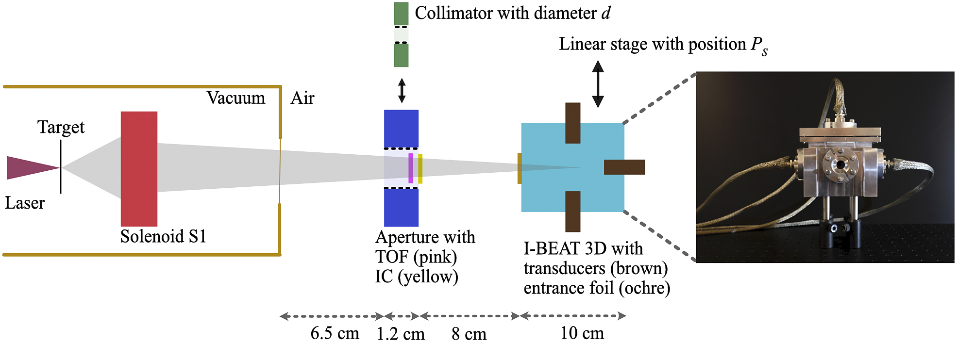
Figure 1 Schematic top view of the experimental setup (not to scale) with all components relevant for this study; in addition, a picture of the I-BEAT 3D detector is shown with the circular entrance window being visible in the centre of the detector. The laser (magenta) is focused onto a thin foil target (black) from which protons are accelerated (grey). One energy selective solenoid S1 focuses the protons to a spot in air. The protons pass either an aperture equipped with a time-of-flight spectrometer (TOF, pink) and an ionization chamber (IC, yellow), or a collimator with a variable diameter (green). Finally, the protons reach the I-BEAT 3D detector, which is positioned on a linear stage. I-BEAT 3D consists of a water reservoir (turquoise) surrounded by four ultrasonic transducers (brown, three are visible). The ions enter the water through a thin Kapton entrance foil (ochre).
Here we present an extension to I-BEAT 3D for analysing particle bunch properties in three dimensions. I-BEAT 3D is equipped with three additional transducers for improving the sensitivity to lateral bunch properties. Using simplified but fast filtered raw data analysis, this setup allows monitoring of the proton bunch mean energy and energy width, lateral position and lateral size as well as the bunch particle number directly from the four acoustic traces.
2 Materials and methods
2.1 Experimental setup
Figure 1 shows the experimental setup that is implemented at the ALBUS-2S ion irradiation beamline of the DRACO laser at Helmholtz-Zentrum Dresden-Rossendorf (HZDR Dresden)[ Reference Brack, Kroll, Gaus, Bernert, Beyreuther, Cowan, Karsch, Kraft, Kunz-Schughart, Lessmann, Metzkes-Ng, Obst-Huebl, Pawelke, Rehwald, Schlenvoigt, Schramm, Sobiella, Szabó, Ziegler and Zeil8]. We operated solenoid S1 to select a small energy range around a design energy value between 13 and 31 MeV from the broad spectrum of laser-accelerated protons, which reached up to 54 MeV. Information on the bunch manipulation by the solenoids can be found in Ref. [Reference Brack, Kroll, Gaus, Bernert, Beyreuther, Cowan, Karsch, Kraft, Kunz-Schughart, Lessmann, Metzkes-Ng, Obst-Huebl, Pawelke, Rehwald, Schlenvoigt, Schramm, Sobiella, Szabó, Ziegler and Zeil8] along with an example of the transported spectrum. After exiting the vacuum chamber, the bunch travels through an air gap of 6.5 cm in length. Then, the proton bunch passes either an aperture equipped with a time-of-flight (TOF) spectrometer[ Reference Kroll, Brack, Bernert, Bock, Bodenstein, Brüchner, Cowan, Gaus, Gebhardt, Helbig, Karsch, Kluge, Kraft, Krause, Lessmann, Masood, Meister, Metzkes-Ng, Nossula, Pawelke, Pietzsch, Püschel, Reimold, Rehwald, Richter, Schlenvoigt, Schramm, Umlandt, Ziegler, Zeil and Beyreuther11, Reference Reimold, Assenbaum, Bernert, Beyreuther, Brack, Karsch, Kraft, Kroll, Loeser, Nossula, Pawelke, Püschel, Schlenvoigt, Schramm, Umlandt, Zeil, Ziegler and Metzkes-Ng19, Reference Scuderi, Milluzzo, Doria, Alejo, Amico, Booth, Cuttone, Green, Kar, Korn, Larosa, Leanza, Martin, McKenna, Padda, Petringa, Pipek, Romagnani, Romano, Russo, Schillaci, Cirrone, Margarone and Borghesi20] and a parallel plate ionization chamber (IC, X-Ray Therapy Monitor Chamber 7862, PTW Freiburg) positioned behind the aperture connected to a dosemeter (UNIDOS, PTW Freiburg) to deduce the proton bunch particle number or a collimator of variable diameter between 1 and 5 mm. The bunch then enters the I-BEAT 3D detector, which is positioned 8 cm behind the aperture or the collimator, respectively. To allow accurate lateral shifts in the horizontal direction relative to the proton axis, the I-BEAT 3D detector is positioned on a motorized stage. I-BEAT 3D consists of an aluminium box with dimensions of 16 cm × 14 cm × 10 cm filled with water into which protons enter through a 50 μm thin Kapton entrance window. While the previous I-BEAT detector was equipped with only one ultrasonic transducer[ Reference Haffa, Yang, Bin, Lehrack, Brack, Ding, Englbrecht, Gao, Gebhard, Gilljohann, Götzfried, Hartmann, Herr, Hilz, Kraft, Kreuzer, Kroll, Lindner, Metzkes-Ng, Ostermayr, Ridente, Rösch, Schilling, Schlenvoigt, Speicher, Taray, Würl, Zeil, Schramm, Karsch, Parodi, Bolton, Assmann and Schreiber17] positioned on the proton axis, the I-BEAT 3D design has four transducers chosen out of the Videoscan series, Olympus Deutschland GmbH. This series offers immersion transducers with various properties, particularly a variable frequency response represented by a central frequency. Furthermore, transducers with flat and spherical sensitive surfaces are available; the latter kind is further referred to as focused. One transducer is mounted in extension of the proton bunch axis (‘axial transducer’, 10 MHz central frequency, 2.54 cm focal length) and has a distance of 3 cm to the entrance window. The three lateral transducers are installed to the right (1 MHz, flat), left (1 MHz, flat) and top (3.5 MHz, 2.54 cm focal length) of the water volume. We chose transducers with lower central frequency for the lateral positions to account for the difference in the frequency spectrum of the acoustic wave at the lateral and axial transducer positions. This is due to the expected sharper gradient in energy deposition in the axial extent of the Bragg peak (BP). It is expected that the central frequency of the transducer influences the deduction of the lateral bunch width. To investigate this, transducers with two different central frequencies are picked for the right/left and top positions. While the top and the axial transducers are chosen to be focused for the optimal signal amplitude, the right and the left transducers are flat to support the scan of the lateral bunch position. For the study presented here, I-BEAT 3D is aligned such that the BP of 30 MeV protons is in the centre of the four transducers (besides when varying the lateral position of the detector relative to the bunch). The distance of each transducer to this design centre is 2.54 cm, which corresponds to the focal length of the axial and the top transducers. The signal of each transducer is 60 dB, amplified by a commercial low-noise amplifier (HVA-10M-60-B, Femto Messtechnik GmbH).

Figure 2 Exemplary ionoacoustic signal recorded with the (a) axial transducer and (b) the right lateral transducer. Curves represent the lowpass filtered data (red, cut-off frequencies: ${f}_{\max, \mathrm{ax}}=4$
MHz for the axial transducer and
${f}_{\max, \mathrm{ax}}=4$
MHz for the axial transducer and ${f}_{\max, \mathrm{lr}}=1$
MHz for the right transducer) and the signal envelope (black). The read-out positions for the deduction of the bunch properties from the signal envelope are marked by dashed lines. For the axial transducer, the arrival time difference between the first and the third maxima corresponds to twice the proton bunch range
${f}_{\max, \mathrm{lr}}=1$
MHz for the right transducer) and the signal envelope (black). The read-out positions for the deduction of the bunch properties from the signal envelope are marked by dashed lines. For the axial transducer, the arrival time difference between the first and the third maxima corresponds to twice the proton bunch range ${R}_{\mathrm{ax}}$
, the pulse width
${R}_{\mathrm{ax}}$
, the pulse width ${w}_{\mathrm{ax}}$
is related to the width of the BP and the amplitude
${w}_{\mathrm{ax}}$
is related to the width of the BP and the amplitude ${A}_{\mathrm{ax}}$
reveals the bunch particle number. For the lateral transducers, the position of the maximum
${A}_{\mathrm{ax}}$
reveals the bunch particle number. For the lateral transducers, the position of the maximum ${P}_{\mathrm{lat}}$
is used to define the lateral bunch position and the pulse width
${P}_{\mathrm{lat}}$
is used to define the lateral bunch position and the pulse width ${w}_{\mathrm{lat}}$
relates to the lateral bunch diameter.
${w}_{\mathrm{lat}}$
relates to the lateral bunch diameter.
2.2 Data analysis
The duration of the proton bunch at the detector position is of the order of tens of ns, which is much smaller than the stress confinement time[
Reference Askariyan, Dolgoshein, Kalinovsky and Mokhov21] that is typically a few μs. In this case, the initial pressure is the product of the energy density distribution deposited by the protons and the material-dependent Grüneisen parameter, which relates energy density to pressure. The propagating pulse amplitude is proportional to the spatial derivative of this initial pressure. Hence, if the deposited energy distribution exhibits only a single spike, such as the BP of focused protons, we expect a single-cycle pulse with a central wavelength and a pulse duration proportional to the size of the distribution in the respective direction of observation. As the phase and amplitude of the acoustic signal will be modified on detection, depending on the spatial and impulse response of the complete geometry and amplifier system[
Reference Wieser, Dash, Savoia, Assmann, Parodi and Lascaud22], we restrict the analysis to the signal envelope calculated by taking the absolute value of the signals’ Hilbert transformation and deduce the amplitudes with their respective positions as well as their full width at half maximum (FWHM) values. Figure 2 shows an exemplary signal for both the axial and the right lateral transducers. The $t$
= 0 μs position corresponds to the time when the laser interacts with the target. The red curves show the single-cycle nature of the pressure pulses and the black curves show the amplitude envelopes. The envelopes recorded with the axial transducer are used to deduce the axial proton bunch properties, while the envelopes from the lateral transducers are employed to measure the lateral bunch properties. All data presented in this study are recorded using individual proton bunches: no averaging is performed. For all transducers, the measured data is filtered with a Butterworth lowpass filter (sixth-order) with cut-off frequencies of
$t$
= 0 μs position corresponds to the time when the laser interacts with the target. The red curves show the single-cycle nature of the pressure pulses and the black curves show the amplitude envelopes. The envelopes recorded with the axial transducer are used to deduce the axial proton bunch properties, while the envelopes from the lateral transducers are employed to measure the lateral bunch properties. All data presented in this study are recorded using individual proton bunches: no averaging is performed. For all transducers, the measured data is filtered with a Butterworth lowpass filter (sixth-order) with cut-off frequencies of ${f}_{\max, \mathrm{ax}}=4$
MHz (axial transducer),
${f}_{\max, \mathrm{ax}}=4$
MHz (axial transducer), ${f}_{\max, \mathrm{top}}=1.5$
MHz (top transducer) and
${f}_{\max, \mathrm{top}}=1.5$
MHz (top transducer) and ${f}_{\max, \mathrm{lr}}=1$
MHz (right and left transducers) to reduce noise.
${f}_{\max, \mathrm{lr}}=1$
MHz (right and left transducers) to reduce noise.
2.2.1 Axial transducer signal
The axial signal in Figure 2(a) reveals three temporally separated pulses that are typical for proton bunches with narrow energy spread[
Reference Assmann, Kellnberger, Reinhardt, Lehrack, Edlich, Thirolf, Moser, Dollinger, Omar, Ntziachristos and Parodi14]: the first one corresponds to the acoustic wave emitted from the BP directly towards the axial transducer. Likewise, an acoustic pulse is emitted from the BP location in the opposite direction towards the entrance foil, where it is reflected and propagates towards the axial transducer, leading to the third peak. The arrival time difference between both pulse envelope maxima, marked by the vertical magenta lines, corresponds to twice the proton bunch range ${R}_{\mathrm{ax}}$
divided by the speed of sound. Using the exponential range–energy relationship[
Reference Bortfeld23], the mean energy
${R}_{\mathrm{ax}}$
divided by the speed of sound. Using the exponential range–energy relationship[
Reference Bortfeld23], the mean energy $E$
of the particle bunch before entering the detector can be deduced[
Reference Lehrack, Assmann, Bertrand, Henrotin, Herault, Heymans, Stappen, Thirolf, Vidal, de Walle and Parodi24].
$E$
of the particle bunch before entering the detector can be deduced[
Reference Lehrack, Assmann, Bertrand, Henrotin, Herault, Heymans, Stappen, Thirolf, Vidal, de Walle and Parodi24].
The width of the pulse ${w}_{\mathrm{ax}}$
is related to the width of the BP
${w}_{\mathrm{ax}}$
is related to the width of the BP ${w}_{\mathrm{BP}}$
. As a measure for this pulse width, we choose the FWHM of the signal envelope (blue vertical lines) multiplied by the speed of sound in water and refer to this as the axial signal width. We assume the following
${w}_{\mathrm{BP}}$
. As a measure for this pulse width, we choose the FWHM of the signal envelope (blue vertical lines) multiplied by the speed of sound in water and refer to this as the axial signal width. We assume the following
 $$\begin{align}{w}_{\mathrm{ax}}=\sqrt{k_{\mathrm{ax}}\cdot {w}_{\mathrm{BP}}^2+{w}_{\mathrm{min}}^2}\end{align}$$
results from the convolution of the axial energy density distribution with width ${w}_{\mathrm{BP}}$
and the shortest possible acoustic pulse
${w}_{\mathrm{BP}}$
and the shortest possible acoustic pulse ${w}_{\mathrm{min}}$
related to the minimal measurable wavelength
${w}_{\mathrm{min}}$
related to the minimal measurable wavelength ${\lambda}_{\mathrm{min}}={c}_{\mathrm{s}}/{f}_{\max, \mathrm{ax}}=0.38$
mm. Thereby,
${\lambda}_{\mathrm{min}}={c}_{\mathrm{s}}/{f}_{\max, \mathrm{ax}}=0.38$
mm. Thereby, ${c}_{\mathrm{s}}$
is the speed of sound in water and
${c}_{\mathrm{s}}$
is the speed of sound in water and ${f}_{\max, \mathrm{ax}}$
is the maximum detectable frequency defined by the lowpass filter. The factor
${f}_{\max, \mathrm{ax}}$
is the maximum detectable frequency defined by the lowpass filter. The factor ${k}_{\mathrm{ax}}$
accounts for a proportional relationship between the BP width and the width of the pressure wave and depends on the shape of the exact distribution function. Based on previous work[
Reference Bortfeld23], the dependence of the BP width on bunch energy
${k}_{\mathrm{ax}}$
accounts for a proportional relationship between the BP width and the width of the pressure wave and depends on the shape of the exact distribution function. Based on previous work[
Reference Bortfeld23], the dependence of the BP width on bunch energy $E$
can be modelled by
$E$
can be modelled by ${w}_{\mathrm{BP}}^2\propto {\sigma}_{\mathrm{E}}^2{E}^{2p-2}$
with
${w}_{\mathrm{BP}}^2\propto {\sigma}_{\mathrm{E}}^2{E}^{2p-2}$
with ${\sigma}_{\mathrm{E}}$
being the width of the Gaussian energy distribution and the constant
${\sigma}_{\mathrm{E}}$
being the width of the Gaussian energy distribution and the constant $p\approx 1.77$
. In our case, the proton bunch energy spread is large and thus it dominates the BP width. The range straggling of a monoenergetic bunch caused by scattering of the protons in water is neglected. The energy spread of the proton bunch focused by the solenoid
$p\approx 1.77$
. In our case, the proton bunch energy spread is large and thus it dominates the BP width. The range straggling of a monoenergetic bunch caused by scattering of the protons in water is neglected. The energy spread of the proton bunch focused by the solenoid ${\sigma}_{\mathrm{E}}$
is first-order proportional to the mean energy,
${\sigma}_{\mathrm{E}}$
is first-order proportional to the mean energy, ${\sigma}_{\mathrm{E}}\propto E$
. Therefore,
${\sigma}_{\mathrm{E}}\propto E$
. Therefore,
 $$\begin{align}{w}_{\mathrm{ax}}=\sqrt{{\tilde{k}}_{\mathrm{ax}}\cdot {E}^{2p}+{w}_{\mathrm{min}}^2}\end{align}$$
is expected to depend on energy.
The second pulse that appears in the centre of the signal trace is generated at the location of the entrance foil. We will show that this signal, in particular the amplitude of its envelope ${A}_{\mathrm{ax}}$
, contains information on the particle number of the proton bunch. This is also true for the first pulse; however, the amplitude of the first pulse is heavily dependent on the energy spread, which makes reconstruction more difficult and less robust. At the entrance window, both mass density and hence deposited energy density as well as the Grüneisen parameter change suddenly. This causes a strongly localized gradient in the initial pressure, which causes the ionoacoustic signal. The ionoacoustic signal amplitude generated at the entrance window location is proportional to the number of protons per area, that is, the proton fluence, as long as the bunch duration is much shorter than the period of the registered acoustic pulse. If, in addition, the detection geometry and the spatial distribution remain constant from bunch to bunch, this amplitude could be a measure for the number of protons contained in a single bunch.
${A}_{\mathrm{ax}}$
, contains information on the particle number of the proton bunch. This is also true for the first pulse; however, the amplitude of the first pulse is heavily dependent on the energy spread, which makes reconstruction more difficult and less robust. At the entrance window, both mass density and hence deposited energy density as well as the Grüneisen parameter change suddenly. This causes a strongly localized gradient in the initial pressure, which causes the ionoacoustic signal. The ionoacoustic signal amplitude generated at the entrance window location is proportional to the number of protons per area, that is, the proton fluence, as long as the bunch duration is much shorter than the period of the registered acoustic pulse. If, in addition, the detection geometry and the spatial distribution remain constant from bunch to bunch, this amplitude could be a measure for the number of protons contained in a single bunch.
2.2.2 Lateral transducer signal
Figure 2(b) shows a typical lateral signal recorded with the right transducer. At $t$
= 0 μs, the measurement shows the decaying EMP contribution generated during laser–plasma interaction; at around 20 μs and thus well separated from the EMP contribution, the acoustic pulse due to the transverse energy density distribution is visible. The lateral bunch position and size can be deduced from this pulse envelope through the maximum position and the FWHM. The left transducer contributes complementary information and, in combination, the right and left transducers allow a cross-check of the extracted parameters for the horizontal bunch position and size. The top transducer signal is analysed in the same way and provides information in the vertical dimension. Finally, we define the lateral bunch position by the time of the envelope maximum (magenta vertical line) multiplied by the speed of sound in water. The FWHM of the lateral ionoacoustic signal envelope
$t$
= 0 μs, the measurement shows the decaying EMP contribution generated during laser–plasma interaction; at around 20 μs and thus well separated from the EMP contribution, the acoustic pulse due to the transverse energy density distribution is visible. The lateral bunch position and size can be deduced from this pulse envelope through the maximum position and the FWHM. The left transducer contributes complementary information and, in combination, the right and left transducers allow a cross-check of the extracted parameters for the horizontal bunch position and size. The top transducer signal is analysed in the same way and provides information in the vertical dimension. Finally, we define the lateral bunch position by the time of the envelope maximum (magenta vertical line) multiplied by the speed of sound in water. The FWHM of the lateral ionoacoustic signal envelope ${w}_{\mathrm{lat}}$
(blue vertical lines) is related to the bunch diameter in the water, which is connected to the collimator size
${w}_{\mathrm{lat}}$
(blue vertical lines) is related to the bunch diameter in the water, which is connected to the collimator size $d$
. As for the axial signal width, we propose the following
$d$
. As for the axial signal width, we propose the following
 $$\begin{align}{w}_{\mathrm{lat}}=\sqrt{k_{\mathrm{lat}}\cdot {d}^2+{w}_0^2}\end{align}$$
by virtue of a convolution of the collimator size $d$
and the shortest possible acoustic pulse with length
$d$
and the shortest possible acoustic pulse with length ${w}_0$
determined by the minimal measurable wavelength plus a potential contribution from lateral broadening during propagation from the collimator to the water and lateral straggling. Again, the constant
${w}_0$
determined by the minimal measurable wavelength plus a potential contribution from lateral broadening during propagation from the collimator to the water and lateral straggling. Again, the constant ${k}_{\mathrm{lat}}$
accounts for the proportionality of the lateral width of the proton bunch to the width of the pressure pulse.
${k}_{\mathrm{lat}}$
accounts for the proportionality of the lateral width of the proton bunch to the width of the pressure pulse.
3 Results
3.1 Axial bunch properties
Figure 3(a) shows the range ${R}_{\mathrm{ax}}$
deduced from the axial I-BEAT 3D signal and the related proton bunch mean energy for five different values of the solenoid magnetic field representing the machine parameter defining the design energy. In addition, the TOF result is shown in blue. For a magnetic field of 11.4 T (13.8 T), two (three) shots were performed that yielded very similar results in terms of mean energy and thus are hardly visible in the figure. For direct comparison between the TOF and I-BEAT 3D, one must account for energy loss in material between both detectors. For that, the IC, the air gap between the TOF and I-BEAT 3D and the I-BEAT 3D entrance window are considered in the reconstruction of the TOF mean energy. The TOF, IC and I-BEAT 3D results are available on the same shot level since the TOF and IC are both transmissive diagnostics. The uncertainty of the magnetic field is dominated by the accuracy of the Rogowski measurement of the solenoid current, which is 0.3% (not visible). The mean energy determined using the I-BEAT 3D detector has an uncertainty defined by the position of the envelope maxima given by half the minimal resolvable wavelength
${R}_{\mathrm{ax}}$
deduced from the axial I-BEAT 3D signal and the related proton bunch mean energy for five different values of the solenoid magnetic field representing the machine parameter defining the design energy. In addition, the TOF result is shown in blue. For a magnetic field of 11.4 T (13.8 T), two (three) shots were performed that yielded very similar results in terms of mean energy and thus are hardly visible in the figure. For direct comparison between the TOF and I-BEAT 3D, one must account for energy loss in material between both detectors. For that, the IC, the air gap between the TOF and I-BEAT 3D and the I-BEAT 3D entrance window are considered in the reconstruction of the TOF mean energy. The TOF, IC and I-BEAT 3D results are available on the same shot level since the TOF and IC are both transmissive diagnostics. The uncertainty of the magnetic field is dominated by the accuracy of the Rogowski measurement of the solenoid current, which is 0.3% (not visible). The mean energy determined using the I-BEAT 3D detector has an uncertainty defined by the position of the envelope maxima given by half the minimal resolvable wavelength ${\lambda}_{\mathrm{min}}/2$
with
${\lambda}_{\mathrm{min}}/2$
with ${\lambda}_{\mathrm{min}}={c}_{\mathrm{s}}/{f}_{\max, \mathrm{ax}}$
. The energy uncertainty is then
${\lambda}_{\mathrm{min}}={c}_{\mathrm{s}}/{f}_{\max, \mathrm{ax}}$
. The energy uncertainty is then $\Delta E=(\mathrm{d}E/\mathrm{d}R)\cdot {\lambda}_{\mathrm{min}}/2$
. The uncertainty of the TOF measurement is determined in the reconstruction process accounting for the complete detector response. The corrected TOF and I-BEAT 3D mean energy match within the uncertainties and absolute deviations remain below 0.8 MeV.
$\Delta E=(\mathrm{d}E/\mathrm{d}R)\cdot {\lambda}_{\mathrm{min}}/2$
. The uncertainty of the TOF measurement is determined in the reconstruction process accounting for the complete detector response. The corrected TOF and I-BEAT 3D mean energy match within the uncertainties and absolute deviations remain below 0.8 MeV.
Figure 3(b) shows the I-BEAT 3D signal width ${w}_{\mathrm{ax}}$
for the same shots as in Figure 3(a) and the fit according to Equation (1). The data points are displayed as a function of the estimated mean bunch energy. The uncertainty for the axial signal width is calculated using Gaussian error propagation, again assuming that
${w}_{\mathrm{ax}}$
for the same shots as in Figure 3(a) and the fit according to Equation (1). The data points are displayed as a function of the estimated mean bunch energy. The uncertainty for the axial signal width is calculated using Gaussian error propagation, again assuming that ${\lambda}_{\mathrm{min}}/2={c}_{\mathrm{s}}/\left(2\cdot {f}_{\max, \mathrm{ax}}\right)$
is the dominating uncertainty. With increasing energy, the I-BEAT 3D signal width rises with the expected parabolic behaviour. The fit parameter
${\lambda}_{\mathrm{min}}/2={c}_{\mathrm{s}}/\left(2\cdot {f}_{\max, \mathrm{ax}}\right)$
is the dominating uncertainty. With increasing energy, the I-BEAT 3D signal width rises with the expected parabolic behaviour. The fit parameter ${\tilde{k}}_{\mathrm{ax}}$
is
${\tilde{k}}_{\mathrm{ax}}$
is $\left(1.5\pm 0.1\right)\times {10}^{-5}\ {\mathrm{mm}}^2\ {\mathrm{MeV}}^{-2p}$
. The minimal measurable signal width
$\left(1.5\pm 0.1\right)\times {10}^{-5}\ {\mathrm{mm}}^2\ {\mathrm{MeV}}^{-2p}$
. The minimal measurable signal width ${w}_{\mathrm{min}}=0.53\pm 0.07$
mm is slightly larger than the minimal resolvable wavelength
${w}_{\mathrm{min}}=0.53\pm 0.07$
mm is slightly larger than the minimal resolvable wavelength ${\lambda}_{\mathrm{min}}=0.38$
mm.
${\lambda}_{\mathrm{min}}=0.38$
mm.

Figure 3 (a) Estimated mean energy and range as a function of the solenoid magnetic field for I-BEAT 3D (black) and TOF (blue). (b) I-BEAT 3D signal width as a function of the determined I-BEAT 3D mean energy. A fit of the I-BEAT 3D data dots according to Equation (2) is shown in green.

Figure 4 (a) I-BEAT 3D result of the bunch position in dependence of the stage position. The resolution limit is shown in red. (b) Measured lateral signal size in dependence of the collimator size along with a fit according to Equation (3) for the top and the right transducers. The minimal measurable pulse width ${w}_0$
is found to be
${w}_0$
is found to be $2.8\pm 0.2$
mm for the right transducer and
$2.8\pm 0.2$
mm for the right transducer and $2.1\pm 0.2$
mm for the top transducer.
$2.1\pm 0.2$
mm for the top transducer.
3.2 Lateral bunch properties
Figure 4 shows the lateral bunch position estimated from the I-BEAT 3D signal. The spatial resolution limit calculated by $\pm {\lambda}_{\mathrm{min}}/(2\cdot \mathrm{SNR})$
is represented by the red lines around the expected curve, for which the I-BEAT 3D bunch position
$\pm {\lambda}_{\mathrm{min}}/(2\cdot \mathrm{SNR})$
is represented by the red lines around the expected curve, for which the I-BEAT 3D bunch position ${P}_{\mathrm{lat}}$
is equal to the nominal bunch position defined by the stage position
${P}_{\mathrm{lat}}$
is equal to the nominal bunch position defined by the stage position ${P}_{\mathrm{S}}$
. SNR is the signal-to-noise ratio. The theoretical resolution limit describes the ability to distinguish two signals, accounting for the limited detector bandwidth. Deviations between the I-BEAT 3D bunch position and nominal bunch position are below 0.4 mm. This data set is recorded with the 3 mm collimator in front of the I-BEAT 3D detector. The uncertainty of the I-BEAT 3D bunch position is given by
${P}_{\mathrm{S}}$
. SNR is the signal-to-noise ratio. The theoretical resolution limit describes the ability to distinguish two signals, accounting for the limited detector bandwidth. Deviations between the I-BEAT 3D bunch position and nominal bunch position are below 0.4 mm. This data set is recorded with the 3 mm collimator in front of the I-BEAT 3D detector. The uncertainty of the I-BEAT 3D bunch position is given by ${\lambda}_{\mathrm{min}}/2$
, which is much larger than the uncertainty of the proton bunch position in the detector and is chosen more conservatively than the theoretical resolution limit. To have a hint as to the reproducibility of the measurement, for some positions several shots were collected. The two consecutive shots at 3 mm and three shots taken at –0.75 mm reveal that shot-to-shot fluctuations cause differences that are smaller than this uncertainty. Accounting for the error bars and the resolution limit, the estimated and the nominal bunch position coincide.
${\lambda}_{\mathrm{min}}/2$
, which is much larger than the uncertainty of the proton bunch position in the detector and is chosen more conservatively than the theoretical resolution limit. To have a hint as to the reproducibility of the measurement, for some positions several shots were collected. The two consecutive shots at 3 mm and three shots taken at –0.75 mm reveal that shot-to-shot fluctuations cause differences that are smaller than this uncertainty. Accounting for the error bars and the resolution limit, the estimated and the nominal bunch position coincide.
Figure 4(b) shows the width of the ionoacoustic signal ${w}_{\mathrm{lat}}$
measured with the right and top transducers as a function of the collimator size
${w}_{\mathrm{lat}}$
measured with the right and top transducers as a function of the collimator size $d$
. A fit of the data according to Equation (3) is shown in green with a dashed and full line, respectively. Shots were taken for the 2 and 5 mm collimators twice, which yielded similar results with deviations below 0.5 mm. The uncertainties of
$d$
. A fit of the data according to Equation (3) is shown in green with a dashed and full line, respectively. Shots were taken for the 2 and 5 mm collimators twice, which yielded similar results with deviations below 0.5 mm. The uncertainties of ${w}_{\mathrm{lat}}$
are calculated based on Equation (3) using Gaussian error propagation, again with
${w}_{\mathrm{lat}}$
are calculated based on Equation (3) using Gaussian error propagation, again with ${\lambda}_{\mathrm{min}}/2$
as the dominating uncertainty. A clear trend towards a larger signal width with increasing collimator size is visible. According to Equation (3), for very small collimator sizes the signal width is given by
${\lambda}_{\mathrm{min}}/2$
as the dominating uncertainty. A clear trend towards a larger signal width with increasing collimator size is visible. According to Equation (3), for very small collimator sizes the signal width is given by ${w}_0$
, which is found to be
${w}_0$
, which is found to be $2.8\pm 0.2$
mm for the right transducer and
$2.8\pm 0.2$
mm for the right transducer and $2.1\pm 0.2$
mm for the top transducer. Thus, it is considerably larger than the minimal resolvable wavelengths
$2.1\pm 0.2$
mm for the top transducer. Thus, it is considerably larger than the minimal resolvable wavelengths ${\lambda}_{\mathrm{min}}=1.5$
mm and 1 mm, respectively. For
${\lambda}_{\mathrm{min}}=1.5$
mm and 1 mm, respectively. For ${k}_{\mathrm{lat}}$
,
${k}_{\mathrm{lat}}$
, $1.8\pm 0.1$
and
$1.8\pm 0.1$
and $1.4\pm 0.1$
are deduced for the right and top signal, respectively.
$1.4\pm 0.1$
are deduced for the right and top signal, respectively.

Figure 5 The amplitude of the ionoacoustic signal envelope generated in the I-BEAT 3D entrance window is displayed in dependence of charge measured with the ionization chamber for various bunch particle numbers. In addition to the black data dots, the linear correlation curve is shown in green.
3.3 Bunch particle number
Figure 5 shows the amplitude of the window signal ${A}_{\mathrm{ax}}$
as a function of the IC signal recorded on the same shot level. For these measurements, the laser energy was varied between 12 and 30 J in order to cover a wide range of proton numbers at the detector position. The given IC signal is the charge collected on the detector electrodes (without further data processing). However, the relation between deposited energy in the detector volume and the read-out charge at the electrodes could be nonlinear for high particle fluxes[
Reference Esplen, Mendonca and Bazalova-Carter6]. The uncertainty of the I-BEAT 3D signal is given by the noise level in the recorded signal. The correlation between the window signal amplitude in I-BEAT 3D (a measure for the proton fluence) and the IC reading (a measure for the proton number) is, with
${A}_{\mathrm{ax}}$
as a function of the IC signal recorded on the same shot level. For these measurements, the laser energy was varied between 12 and 30 J in order to cover a wide range of proton numbers at the detector position. The given IC signal is the charge collected on the detector electrodes (without further data processing). However, the relation between deposited energy in the detector volume and the read-out charge at the electrodes could be nonlinear for high particle fluxes[
Reference Esplen, Mendonca and Bazalova-Carter6]. The uncertainty of the I-BEAT 3D signal is given by the noise level in the recorded signal. The correlation between the window signal amplitude in I-BEAT 3D (a measure for the proton fluence) and the IC reading (a measure for the proton number) is, with ${R}^2=0.93$
, very high. If both the IC and I-BEAT 3D are ideal detectors and the lateral bunch size is constant, a linear relationship is expected, as discussed in Section 2.2.1.
${R}^2=0.93$
, very high. If both the IC and I-BEAT 3D are ideal detectors and the lateral bunch size is constant, a linear relationship is expected, as discussed in Section 2.2.1.
4 Discussion and conclusion
Equipped with four transducers, the I-BEAT 3D detector provides acoustic traces in four spatial directions. As expected, the analysis of the envelope of the filtered raw signal amplitudes reveals the position and the width of the BP volume. The accuracy of this position is currently limited to the resolution limit of 0.04 mm in the axial dimension and 0.16 mm in the lateral dimension, depending on the maximal detectable frequency and the signal-to-noise ratio. In the axial direction, this analysis yields an absolute measure of the proton range[
Reference Assmann, Kellnberger, Reinhardt, Lehrack, Edlich, Thirolf, Moser, Dollinger, Omar, Ntziachristos and Parodi14,
Reference Lehrack, Assmann, Bertrand, Henrotin, Herault, Heymans, Stappen, Thirolf, Vidal, de Walle and Parodi24] and hence kinetic energy before entering the water reservoir in real-time with an accuracy of 0.8 MeV. Analysis of the width of the signal envelope allows in addition fast monitoring of the width of the BP, which is a measure of the energy spread $\mathrm{d}E/E$
as long as this is larger than 2% and other factors, such as range straggling, can be neglected. Equation (2) describes the relationship between the measured signal width and bunch energy well. The relation between the lateral signal width and aperture diameter is likewise well described by Equation (3). The minimum signal width
$\mathrm{d}E/E$
as long as this is larger than 2% and other factors, such as range straggling, can be neglected. Equation (2) describes the relationship between the measured signal width and bunch energy well. The relation between the lateral signal width and aperture diameter is likewise well described by Equation (3). The minimum signal width ${w}_0$
is smaller for the top transducer than for the right transducer, which is expected due to its larger frequency bandwidth. The difference in
${w}_0$
is smaller for the top transducer than for the right transducer, which is expected due to its larger frequency bandwidth. The difference in ${w}_0$
between the two transducers thus confirms our signal modelling. However, for both lateral signals, the width remains considerably larger than the ultrasound resolution limit though, and straggling within the remaining 8 cm of air after passing the collimator as well as the water cannot account for this. This hints at additional contributions, for example by the vacuum exit window, and deserves further investigation. Employing transducers with a larger bandwidth, increasing the number of transducers[
Reference Kellnberger, Assmann, Lehrack, Reinhardt, Thirolf, Queirós, Sergiadis, Dollinger, Parodi and Ntziachristos25] or utilizing computationally more expensive reconstruction algorithms that take into account the response functions[
Reference Haffa, Yang, Bin, Lehrack, Brack, Ding, Englbrecht, Gao, Gebhard, Gilljohann, Götzfried, Hartmann, Herr, Hilz, Kraft, Kreuzer, Kroll, Lindner, Metzkes-Ng, Ostermayr, Ridente, Rösch, Schilling, Schlenvoigt, Speicher, Taray, Würl, Zeil, Schramm, Karsch, Parodi, Bolton, Assmann and Schreiber17,
Reference Wieser, Dash, Savoia, Assmann, Parodi and Lascaud22] is expected to improve the accuracy of the demonstrated proton bunch monitor.
${w}_0$
between the two transducers thus confirms our signal modelling. However, for both lateral signals, the width remains considerably larger than the ultrasound resolution limit though, and straggling within the remaining 8 cm of air after passing the collimator as well as the water cannot account for this. This hints at additional contributions, for example by the vacuum exit window, and deserves further investigation. Employing transducers with a larger bandwidth, increasing the number of transducers[
Reference Kellnberger, Assmann, Lehrack, Reinhardt, Thirolf, Queirós, Sergiadis, Dollinger, Parodi and Ntziachristos25] or utilizing computationally more expensive reconstruction algorithms that take into account the response functions[
Reference Haffa, Yang, Bin, Lehrack, Brack, Ding, Englbrecht, Gao, Gebhard, Gilljohann, Götzfried, Hartmann, Herr, Hilz, Kraft, Kreuzer, Kroll, Lindner, Metzkes-Ng, Ostermayr, Ridente, Rösch, Schilling, Schlenvoigt, Speicher, Taray, Würl, Zeil, Schramm, Karsch, Parodi, Bolton, Assmann and Schreiber17,
Reference Wieser, Dash, Savoia, Assmann, Parodi and Lascaud22] is expected to improve the accuracy of the demonstrated proton bunch monitor.
Particularly interesting is the observed correlation between the ionoacoustic signal generated in the entrance window of the I-BEAT 3D detector and the IC signal, although the deviations are larger than the individual uncertainties. This hints at the differences due to the physics of the two approaches. While the IC measures the number of charges that is assumed to scale (eventually nonlinear) with the total particle number[ Reference Esplen, Mendonca and Bazalova-Carter6], the ionoacoustic signal depends on the spatial distribution of the bunch that traverses the entrance foil and on the detector geometry. That is, the signal is sensitive to proton bunch fluence, and not just particle number, which can be seen in Equation (1) in Ref. [Reference Haffa, Yang, Bin, Lehrack, Brack, Ding, Englbrecht, Gao, Gebhard, Gilljohann, Götzfried, Hartmann, Herr, Hilz, Kraft, Kreuzer, Kroll, Lindner, Metzkes-Ng, Ostermayr, Ridente, Rösch, Schilling, Schlenvoigt, Speicher, Taray, Würl, Zeil, Schramm, Karsch, Parodi, Bolton, Assmann and Schreiber17]. As an example for a 30 MeV proton bunch, when increasing the lateral signal width from 3 to 3.1 mm, the pressure amplitude is decreased by approximately 5%.
In conclusion, the presented fast and simple data analysis allows monitoring important proton bunch parameters of the focused and energy selected proton bunch in a compact, simple, fast and EMP-resistant online tool. Compared to the previously used simulated annealing approach[ Reference Haffa, Yang, Bin, Lehrack, Brack, Ding, Englbrecht, Gao, Gebhard, Gilljohann, Götzfried, Hartmann, Herr, Hilz, Kraft, Kreuzer, Kroll, Lindner, Metzkes-Ng, Ostermayr, Ridente, Rösch, Schilling, Schlenvoigt, Speicher, Taray, Würl, Zeil, Schramm, Karsch, Parodi, Bolton, Assmann and Schreiber17] demonstrated for dose reconstruction in the axial dimension (i.e., the depth dose curve), the here presented fast data analysis has the advantage that the extraction of information becomes compatible with 1 Hz operation and potentially much higher repetition rates. Having in mind that a full reconstruction of the depth dose curve is possible, for many use cases fast feedback on the energy width of a focused proton bunch is sufficient. The I-BEAT 3D detection method is not only promising as a beam monitor for laser-ion accelerators, but could also be applied for preclinical and clinical research in the context of FLASH radiotherapy[ Reference Esplen, Mendonca and Bazalova-Carter6], as the high dose rates used in this new treatment modality challenge well-established bunch monitoring systems.
Acknowledgements
This work was supported by the German Research Foundation (DFG) within the Research Training Group GRK 2274 and the Bundesministerium für Bildung und Forschung (BMBF) within project 01IS17048. F.B. acknowledges financial support by the BMBF within projects 05P18WMFA1 and 05P21WMFA1. The authors acknowledge J. Lascaud, W. Assmann and H.-P. Wieser for fruitful discussions on the project.


 Open access