3.1 Experimental details of the high-power wavelength-tunable SFS

We first investigated the wavelength-tunable operation of the high-power SFS. The inset of Figure 1(a) shows the output spectrum of the broadband SFS seed, which covers a spectral range of 1060–1115 nm under the measured optical signal-to-noise ratio (OSNR) of 45 dB, and the spectral peak is located at approximately 1080 nm with an FWHM linewidth of approximately 10 nm. Taking the filter passband of 4 nm as an example, the wavelength-tunable spectra after the BA-TOF are shown in Figure 1(b). Note that the seed power decreases dramatically with the filter wavelength deviating from the central peak; to improve the powers of the sideband wavelengths and reduce the amplification ratio of pre-amplifier 1, the filter passband for 1068, 1090, and 1092 nm is increased to 6 nm. Figure 1(c) shows the seed powers with different filter wavelengths. The highest seed power reaches approximately 18.7 mW at 1080 nm, whereas the powers at 1068 and 1092 nm decrease to 1.1 and 2.7 mW, respectively.

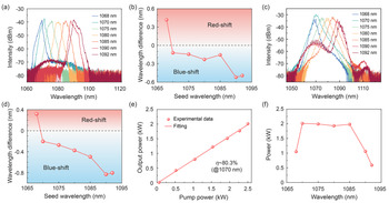
Figure 2(a) depicts the wavelength-tunable spectra after pre-amplifier 2. Unlike the seed spectra with sharp edges, the output spectra of pre-amplifier 2 show considerable spectral broadening. Moreover, due to the relatively low powers of the sideband wavelengths, such as 1068 and 1092  nm, amplified spontaneous emission (ASE) occurs during the amplification process. The intensity difference between the signal peak and the ASE background is approximately 35 dB. In addition, due to the gain competition, a variation in the central wavelengths has been observed^[ Reference Yan, Sun, Li, Gong and Xiao ^{31 –} Reference Yang, Wu, Li, Duan, Liu, Miao and Zhao ^{33 ]}, as presented in Figure  2(b). The wavelength difference Δλ is defined as λ _amp–λ _seed, where λ _amp and λ _seed represent the central wavelengths of pre-amplifier 2 and the filtered seed, respectively. The spectrum at 1068 nm shows a wavelength red-shift of approximately 0.4 nm, whereas the central wavelengths over 1070–1085 nm have no major changes, and the spectra at 1090 and 1092 nm exhibit an obvious blue-shift of approximately 0.5 nm. Figure 2(c) shows the wavelength-tunable spectra after the main amplifier, which are a little spiky due to the intermodal interference of the multi-mode (MM) coupling fiber used in the spectral measurement^[ Reference Hlubina ^{34 ]}. We also analyzed the wavelength variation of the main amplifier, as presented in Figure 2(d), where the wavelength difference Δλ is also defined as λ _amp – λ _seed. Compared with pre-amplifier 2, the main amplifier shows a further wavelength blue-shift. The longer the central wavelength, the more considerable the wavelength variation. For instance, the wavelength blue-shift at the central wavelengths of 1090 and 1092 nm increases to approximately 0.8 nm. The wavelength variation is related to the spectral distribution of the gain coefficient, and the central wavelength will drift towards the region with the maximum gain coefficient. The gain distribution in the spectral domain is dependent on the pump power, fiber parameters and even temperature^[ Reference Yan, Sun, Li, Gong and Xiao ^{31 ,} Reference Wu, Wang, Zhao, Zhao, Miao, Li, Gao and Zheng ^{32 ]}. In our case, the wavelength region with the maximum gain coefficient is located near 1070 nm (according to the ASE background), and thus the spectrum at 1068 nm shows a wavelength red-shift, whereas the central wavelengths over 1070–1085 nm have a small blue-shift and the spectra at 1090 and 1092 nm exhibit a larger blue-shift.

Figure 2 (a) Wavelength-tunable spectra after pre-amplifier 2. The filter passband for 1070–1085 nm is fixed at 4 nm, whereas that for 1068, 1090, and 1092 nm is increased to 6 nm. (b) Central wavelength difference between the output spectra of the filtered seed and pre-amplifier 2. (c) Wavelength-tunable spectra after the main amplifier. (d) Central wavelength difference between the output spectra of the filtered seed and the main amplifier. (e) Power evolution at 1070 nm. (f) Maximum output power as a function of the operating wavelength.

Figure 2(e) shows the power evolution of the main amplifier at the central wavelength of 1070 nm. The maximum output power reaches approximately 2010 W with the injected pump power of 2500 W, corresponding to a slope efficiency of about 80.3%. Figure 2(f) presents the maximum output power as a function of the operating wavelength. The full output power over the wavelength range of 1070–1085 nm exceeds 1930 W. Meanwhile, at 1090 and 1092 nm, due to the considerable growth of ASE light near 1070 nm (as shown in Figure 2(c), the intensity difference between the signal peak and the ASE reduces to below 20 dB), the maximum output power is only amplified to 1060 and 590 W, respectively. In addition, because the seed power is too weak at 1068 nm (~1.1 mW), and to ensure the system safety, the maximum output power at 1068 nm is only scaled to 1050 W.

3.2 Experimental details of the high-power linewidth tunable SFS

We also explored the linewidth tunable operation of the high-power SFS. Taking the central wavelength of 1080 nm as an example, the seed spectra with different filtering passbands are shown in Figure 3(a). The legend represents the FWHM linewidth of the filtered spectrum. Figure 3(b) shows that the seed power increases with the spectral linewidth; the minimum seed power is 4.7 mW whereas the maximum seed power reaches approximately 51.5 mW.

Figure 3 (a) Linewidth tunable spectra after the BA-TDF. The legend represents the FWHM linewidth of the filtered spectrum. (b) Output powers of the filtered SFS seed with different FWHM linewidths.

Figure 4(a) presents the linewidth tunable spectra after pre-amplifier 2. Due to the nonlinear effects, such as self-phase modulation (SPM)^[ Reference Ma, Tao, Wang, Zhou and Liu ^{23 ,} Reference Xu, Ye, Xiao, Leng, Liu and Zhou ^{24 ]}, the optical spectra have different degrees of broadening. Here we introduce a spectral broadening factor, defined as Δλ _out/Δλ _in, where Δλ _out and Δλ _in respectively represent the spectral FWHM linewidth of pre-amplifier 2 and the seed. As shown in Figure 4(b), the broadening factor decreases with the increment of the seed linewidth, indicating that the narrower the input spectrum, the stronger the spectral broadening in the amplifiers. The maximum broadening factor reaches 1.92 with the seed linewidth of 0.5 nm, while with the increasing seed linewidth to more than 4 nm, the broadening factor tends to approximately 1. However, this does not mean that those spectra are unchanged, since spectral broadening of the tails can be observed clearly.

Figure 4 (a) Linewidth tunable spectra after pre-amplifier 2. The legend represents the FWHM linewidth of the filtered SFS seed. (b) Spectral broadening factor as a function of the seed linewidth. (c) Linewidth tunable spectra after the main amplifier. (d) Spectral broadening factors of the main amplifier depending on the output power. (e) Power evolutions with the seed linewidths of 0.5, 4, and 10 nm. (f) Maximum output power of the main amplifier versus the seed linewidth.

The linewidth tunable spectra further broadened after the main amplifier. As presented in Figure 4(c), the FWHM linewidth is tunable over 2.5–9.7 nm. However, it is seen that the spectra after the main amplifier are symmetrical and have long tails, so the FWHM linewidth cannot fully describe the spectral evolution; here, we introduce another parameter, the root-mean-square (RMS) linewidth, to further analyze the spectral broadening^[ Reference Liu, Ma, Zhou and Jiang ^{35 ]}. Figure 4(d) presents the broadening factors of the RMS linewidth as functions of the output power. The spectral evolution is similar to that of the pre-amplifiers, where a narrower seed also shows stronger spectral broadening in the main amplifier; the broadening rate with a 0.5 nm seed linewidth reaches 1.4 kW^–1, while that with 4 and 10 nm seed linewidths decreases to 0.4 and 0.06 kW^–1, respectively. In addition, the seed linewidth has little impact on the power amplification. As shown in Figure  4(e), the power evolutions of the main amplifier with the seed linewidths of 0.5, 4, and 10 nm are nearly identical. Taking the case of 0.5 nm, for example, the maximum output power reaches 1950 W with the pump power of 2500 W, corresponding to a slope efficiency of approximately 78.3%. The maximum output power of the main amplifier as a function of the seed linewidth is plotted in Figure 4(f), showing that the output power over the whole tuning range exceeds 1940 W.

4.1 Theoretical model

To further investigate the generation and amplification of the wavelength and linewidth tunable SFS, especially for establishing the role of gain competition and nonlinear effects, a numerical simulation is conducted based on the combining of rate equations and the GNLSE (see Refs. [Reference Liu, Ma, Zhou and Jiang35–Reference Turitsyn, Bednyakova, Fedoruk, Latkin, Fotiadi, Kurkov and Sholokhov37] for details):

(1) \begin{align}\frac{\partial \tilde{A}\left(z,\omega \right)}{\partial z}&=\frac{1}{2}\left[g\left(z,\omega \right)-\alpha \left(\omega \right)\right]\tilde{A}\left(z,\omega \right) +i\sum \limits_{n=2}^3\frac{\beta_n}{n!}{\omega}^n\tilde{A}\left(z,\omega \right) \notag\\&\quad + i\gamma \left(\omega \right){\left|\tilde{A}\left(z,\omega \right)\right|}^2\tilde{A}\left(z,\omega \right)+{f}_{\mathrm{SEN}}\left(z,\omega \right),\end{align}

(2) \begin{align}\frac{\mathrm{d}{P}_{\mathrm{p}}(z)}{\mathrm{d}z}&=-{\Gamma}_{\mathrm{p}}\left\{{\sigma}_{\mathrm{a}}\left({\omega}_{\mathrm{p}}\right){N}_0- \left[{\sigma}_{\mathrm{a}}\left({\omega}_{\mathrm{p}}\right)+{\sigma}_{\mathrm{e}}\left({\omega}_{\mathrm{p}}\right)\right]{N}_2\right\}\notag\\&\quad\times{P}_{\mathrm{p}}(z)-{\alpha}_{\mathrm{p}}{P}_{\mathrm{p}}(z),\end{align}

(3) \begin{align}&\frac{N_2(z)}{N_0}=\frac{\Gamma_{\mathrm{p}}}{\mathrm{\hslash}{\omega}_{\mathrm{p}}A}{\sigma}_{\mathrm{a}} \left({\omega}_{\mathrm{p}}\right){P}_{\mathrm{p}} \nonumber \\&\quad +\frac{1}{2\pi {T}_{\mathrm{m}}A}\int \frac{\Gamma_{\mathrm{s}}\left(\omega \right)}{\mathrm{\hslash}\omega }{\sigma}_{\mathrm{a}}\left(\omega \right){\left|\tilde{A}\left(z,\omega \right)\right|}^2\mathrm{d}\omega \nonumber \\&\quad \times \left\{ \frac{\Gamma_{\mathrm{p}}}{\mathrm{\hslash}{\omega}_{\mathrm{p}}A}\left[{\sigma}_{\mathrm{a}}\left({\omega}_{\mathrm{p}}\right) +{\sigma}_{\mathrm{e}}\left({\omega}_{\mathrm{p}}\right)\right]{P}_{\mathrm{p}}+\frac{1}{\tau } \right. \nonumber \\&\quad \left. +\frac{1}{2\pi {T}_{\mathrm{m}}A}\int \frac{\Gamma_{\mathrm{s}}\left(\omega \right)}{\mathrm{\hslash}\omega}\left[{\sigma}_{\mathrm{a}}\left(\omega \right)+{\sigma}_{\mathrm{e}}\left(\omega \right)\right]{\left|\tilde{A}\left(z,\omega \right)\right|}^2\mathrm{d}\omega \right\}^{-1},\end{align}

(4) \begin{align}g\left(z,\omega \right)={\Gamma}_{\mathrm{s}}\left(\omega \right)\left\{{N}_2(z)\left[{\sigma}_{\mathrm{e}}\left(\omega \right)+{\sigma}_{\mathrm{a}}\left(\omega \right)\right]-{N}_0{\sigma}_{\mathrm{a}}\left(\omega \right)\right\}.\end{align}

The SFS seed and the amplifiers can be simulated by Equation (1), wherein $\tilde{A}\left(z,\omega \right)$ represents the complex field in the frequency domain, g and α are the active gain and loss coefficients, respectively, β_n represents the nth-order dispersion coefficients, γ is the nonlinear Kerr coefficient, and f _SEN represents the spontaneous emission noise (SEN). For the sake of simplicity, here we have neglected the SRS effect, because it has not been observed in the experiments. Equation (2) describes the evolution of the pump power P _p with the fiber length, where Γ is the overlap factor, σ _a and σ _e represent the absorption and emission cross-sections, respectively, N ₀ is the dopant concentration, N ₂ denotes the number of excited Yb ions, which is governed by Equation (3), τ is the lifespan of the excited state population, ℏ is the reduced Planck constant, and A is the doped cross-section area. The active gain is given by Equation (4), which acts as a bridge between the rate equations and the GNLSE^[ Reference Liu, Ma, Zhou and Jiang ^{35 ,} Reference Liu, Ma, Lv, Xu, Zhou and Jiang ^{36 ]}. The SEN is approximated by a Gaussian random process with zero mean value, which satisfies^[ Reference Liu, Ma, Zhou and Jiang ^{35 ]}

(5) \begin{align}&\left\langle {f}_{\mathrm{SEN}}\left(z,\omega \right){f}_{\mathrm{SEN}}^{\ast}\left(z^{\prime},\omega^{\prime}\right)\right\rangle\notag\\&\quad{}=\frac{\mathrm{\hslash}{\omega}^3}{\pi {c}^2}n\left(\omega \right)g\left(z,\omega \right){n}_{\mathrm{sp}}\delta \left(z-z^{\prime}\right)\delta \left(\omega -\omega^{\prime}\right),\end{align}

(6) \begin{align}{n}_{\mathrm{sp}}=\frac{1}{\exp \left[\frac{\mathrm{\hslash}\left(\omega +{\omega}_0\right)}{k_{\mathrm{B}}T}\right]-1},\end{align}

where n _sp is the average mode occupation number in equilibrium, δ is the Dirac delta function, and k _B and T represent the Boltzmann constant and the temperature, respectively. In addition, the effect of the BA-TOF can be described as

(7) \begin{align}{\tilde{A}}_{\mathrm{out}}\left(\omega \right)={\tilde{A}}_{\mathrm{in}}\left(\omega \right)\sqrt{T_{\mathrm{r}}\left(\omega \right)},\end{align}

where ${\tilde{A}}_{\mathrm{out}}\left(\omega \right)$ and ${\tilde{A}}_{\mathrm{in}}\left(\omega \right)$ are the output and input optical fields and ${T}_{\mathrm{r}}\left(\omega \right)$ represents the transmission spectrum of the filter, which can be approximated by a super-Gaussian function. Furthermore, it is worth noting that the theoretical model is numerically calculated using the well-known split-step Fourier method (SSFM)^[ Reference Turitsyn, Bednyakova, Fedoruk, Latkin, Fotiadi, Kurkov and Sholokhov ^{37 ]}; the parameter values used in the simulation are attached in the Supplementary Materials.

4.2 Simulation of the high-power wavelength-tunable SFS

We first simulated the generation and filtering of the SFS seed, as shown in Figure 5(a); the broadband SFS seed has a relatively sharp spectral edge at the short-wavelength side and a gentle tail at the long-wavelength side, and the 40-dB spectral coverage spans from 1045 to 1145 nm. The filtered spectrum shows a broad pedestal with a sharp peak, where the filtering passband is fixed at 4 nm and the out-band suppression ratio is set to 50 dB. Figures 5(b) and 5(c) present the temporal behaviors of the broadband seed and the filtered signal, respectively, which are normalized by the mean intensities <I(t)>. The temporal profiles exhibit strong fluctuations in the timescale of picoseconds^[ Reference Kelleher, Travers, Popov and Taylor ^{19 ,} Reference Liu, Ma, Lv, Xu, Zhou and Jiang ^{36 ]}, and the peak powers can reach several multiples of the mean value. The fluctuation scale increases after the spectral filtering, which can be verified by the intensity autocorrelation functions (ACFs). As depicted in Figure 5(d), the FWHM of the ACF increases from approximately 100 fs to approximately 0.8 ps after the filtering. In addition, the ACF background remains at 0.5, indicating that the filtering process does not affect the statistical property of the optical field, and the spectral components are still uncorrelated^[ Reference Churkin, Gorbunov and Smirnov ^{38 ]}. We can further verify this result through the intensity probability density functions (PDFs), as shown in Figure 5(e). The intensity PDF after the spectral filtering is the same as that of the broadband seed, and the exponential decay factor of –1 indicates that the optical field can be seen as a Gaussian random process^[ Reference Gorbunov, Sugavanam and Churkin ^{39 ]}. This conclusion is quite beneficial, since we can use the experimental seed spectrum with random phases as the input of the amplifiers, which can further improve the accuracy of the simulation.

Figure 5 (a) Simulated spectra of the unfiltered broadband SFS seed and the filtered SFS seed. Temporal intensity profile of (b) the unfiltered SFS seed and (c) the filtered SFS seed. (d) Intensity autocorrelation functions (ACFs) and (e) intensity probability density functions (PDFs) of the unfiltered SFS seed and the filtered signal. (f) Simulated wavelength-tunable spectra after pre-amplifier 2. (g) Simulated central wavelength difference between the output spectra of the filtered seed and pre-amplifier 2. (h) Simulated wavelength-tunable spectra after the main amplifier. (i) Simulated central wavelength difference between the output spectra of the filtered seed and the main amplifier.

Figure 5(f) illustrates the simulated wavelength-tunable spectra after pre-amplifier 2, which agree well with the experimental results. In addition, due to the uneven spectrum of the filtered seed and the gain competition in the amplifiers, the output spectrum shows a red-shift at the short-wavelength side and a blue-shift at the long-wavelength side. We also calculated the variations of the central wavelength, where the definition of wavelength variation is the same as that in Section 3 . As presented in Figure 5(g), the spectrum at 1068 nm shows a wavelength red-shift of approximately 0.3  nm, whereas the wavelengths over 1070–1085 nm have no great changes and the spectra at 1090 and 1092 nm exhibit an obvious blue-shift of approximately 0.5 nm, which also agrees well with the experimental data. Figure 5(h) shows the simulated wavelength-tunable spectra after the main amplifier, where with tuning the operating wavelength to the longer side, the ASE light grows dramatically. The intensity difference between the signal peak and the ASE reduces to approximately 20 dB at 1092 nm. It is worth noting that the ASE profile in the experiments is a little different from the simulated results, which could be attributed to the four-wave mixing (FWM) effect^[ Reference Xu, Ye, Xiao, Leng, Liu and Zhou ^{24 ]}, and another peak at approximately 1110 nm can be seen as an additional piece of evidence (see Figure 2(c)). We further analyzed the wavelength variation in the main amplifier, as shown in Figure 5(i). The red-shift increases at the short-wavelength side, for example, the spectrum at 1068 nm shows a wavelength red-shift of approximately 0.6 nm after the main amplifier, whereas the central wavelength at the long-wavelength side remains almost unchanged compared with the pre-amplifier. By optimizing the operating temperature and the system parameters, such as fiber length, in the seed and amplifiers^[ Reference Yan, Sun, Li, Gong and Xiao ^{31 ,} Reference Wu, Wang, Zhao, Zhao, Miao, Li, Gao and Zheng ^{32 ,} Reference Liu, Ma, Zhou and Jiang ^{35 ]}, it is possible to further suppress the ASE light, reduce the wavelength variation and increase the wavelength tunable range.

4.3 Simulation of the high-power linewidth tunable SFS

We also simulated the linewidth tunable operation of the SFS. Figure 6(a) shows the linewidth tunable spectra after pre-amplifier 2. Compared with the filtered spectra of the seed (Figure 3(a)), a noticeable broadening of the spectral tails can be observed. The spectral broadening factors calculated using the RMS and FWHM linewidth are presented in Figure 6(b). With the same initial seed linewidth, the broadening factor of the RMS linewidth is larger than that of the FWHM linewidth, because the RMS linewidth takes into account the spectral tails whereas the FWHM linewidth is only concerned with the spectral peak. In addition, both the evolution trends are similar, that is, the broader the initial seed linewidth, the smaller the broadening factors, which is qualitatively matched with the experimental results. The maximum broadening factors of the RMS and FWHM linewidths reach 2.3 and 1.4, respectively, with the initial seed linewidth of 0.5 nm, whereas with increasing the seed linewidth to 10 nm, the broadening factors of the RMS and FWHM linewidths decrease to 0.92 and 0.84, respectively, indicating that the amplified SFS has a narrower spectrum than the SFS seed. Figure 6(c) shows the linewidth tunable spectra after the main amplifier. The output spectrum further broadens due to the nonlinear effects, such as SPM. However, the simulated output spectrum with a narrowband seed is much broader than the experimental result. For example, the simulated FWHM linewidth with 2 nm initial seed linewidth reaches 4.6 nm, whereas the experimental value is 2.6 nm. This deviation may be attributed to the simulation model of the main amplifier, since it does not take into account the transverse modes, and the existence of MMs could bring additional dispersion, intermodal dispersion^[ Reference Kubota, Takara, Nakagawa, Matsui and Morioka ^{40 ]}, further affecting the interplay of dispersion and nonlinearity; thus, the experimental output spectra are narrower than the simulated ones (with narrowband seed spectra). Future research may employ the generalized multimode nonlinear Schrödinger equations (GMMNLSEs) to improve simulation accuracy^[ Reference Wright, Ziegler, Lushnikov, Zhu, Eftekhar, Christodoulides and Wise ^{41 ]}. Despite the deviation, we also calculated the broadening factor of the RMS and FWHM linewidths after the main amplifier, as shown in Figure 6(d). The evolution trend is similar to that of pre-amplifier 2. The broader the initial seed linewidth, the smaller the broadening factors.

Figure 6 (a) Simulated linewidth tunable spectra after pre-amplifier 2. (b) Broadening factors of the spectral width versus the seed linewidth (after pre-amplifier 2). (c) Simulated linewidth tunable spectra after the main amplifier. (d) Broadening factors of the spectral width after the main amplifier depending on the seed linewidth. (e), (f) Simulated output spectra of the main amplifier with and without Kerr nonlinearity (initial seed linewidth: (e) 0.5 nm; (f) 8 nm). The output spectrum of pre-amplifier 2 is also provided for the sake of comparison.

To further establish the limiting factors of the linewidth tuning range, we investigated the impacts of nonlinear effects and gain competition. By setting the nonlinear Kerr coefficient γ as 0, we can independently explore the influence of gain competition. Figure 6(e) shows the simulated output spectra of the main amplifier with γ = 0.5 W^–1 $\cdot$ km^–1 and without Kerr nonlinearity (γ = 0), in which the initial seed linewidth is 0.5 nm. Compared with the output spectrum of pre-amplifier 2, the output spectrum of the main amplifier without Kerr nonlinearity shows a lower ASE background, indicating that the signal peak obtains more gain in the amplification process. In addition, the spectral linewidth is almost the same as that of pre-amplifier 2 (see the yellow and blue lines in Figure 6(e)). While taking into account the Kerr nonlinearity, the spectrum shows considerable broadening both in the peak and tails (see the red line in Figure 6(e)), so we can conclude that the lower limit of the linewidth tuning range is mainly limited by the SPM effect^[ Reference Xu, Ye, Xiao, Leng, Liu and Zhou ^{24 ]}.

Furthermore, we simulated the impact of nonlinear effects and gain competition on the final output spectrum with the seed linewidth of 8 nm. As shown in Figure 6(f), in contrast to the case with 0.5 nm seed linewidth, the output spectrum of the main amplifier without Kerr nonlinearity shows a higher ASE background. In addition, the spectral linewidth broadens a little compared with that of pre-amplifier 2; specifically, the RMS linewidth broadens from 5.1 to 5.2  nm and the FWHM linewidth increases from 6.0 to 6.6 nm, indicating that the gain competition reshapes the spectral profile and results in a relatively flatter output spectrum^[ Reference Yan, Sun, Li, Gong and Xiao ^{31 ,} Reference Wu, Wang, Zhao, Zhao, Miao, Li, Gao and Zheng ^{32 ]}. However, the nonlinear effects further change the spectral profile, where the simulated output spectrum of the main amplifier with Kerr nonlinearity is quite symmetric and the RMS and FWHM linewidths are calculated to be 6.0 and 5.7 nm, respectively. Here we would like to discuss the spectral evolution and the underlying physical mechanism briefly. In general, the gain competition usually reshapes the optical spectrum, resulting in spectral narrowing or spectral broadening (depending on whether the spectral peak can obtain more gain than other components). The SPM effect is responsible for the spectral broadening, whereas the inverse four-wave mixing (IFWM) effect may contribute to the spectral narrowing. The IFWM is a new nonlinear self-action effect that may occur in the normal dispersion regime and lead to the spectral compression^[ Reference Turitsyn, Bednyakova, Fedoruk, Papernyi and Clements ^{42 ]}. In our case, the increase of RMS linewidth indicates that the spectral tails have broadened due to the SPM effect, while the decrease of FWHM linewidth may be attributed to the IFWM effect^[ Reference Zhang, Bai, Li, Yang, He and Zhou ^{43 ,} Reference Ye, Ma, Zhang, Xu, Zhang, Yao, Leng and Zhou ^{44 ]}. Thus, the lower limit of the linewidth tuning range is mainly affected by the SPM effect and the upper limit of the linewidth tuning range is defined by the combined effect of gain competition and nonlinear effects (such as SPM and IFWM effects).