


Social media summary
Earth3 global simulation model enables option exploration to achieve all 17 SDGs within planetary boundaries: extraordinary action needed.
1. Introduction
Seventeen global Sustainable Development Goals were agreed by the UN in 2015, with the ambition to achieve them by 2030. Our focus is the apparent conflict between the three ‘environmental’ goals (SDGs 13, 14 and 15) and the 14 ‘socio-economic’ goals. Griggs et al. (Reference Griggs, Stafford-Smith, Gaffney, Rockström, Öhman, Shyamsundar and Noble2013) pointed out the need to give priority to the environmental goals: ‘so that today's advances in development are not lost as our planet ceases to function for the benefit of a global population’. Efforts to achieve the 14 socio-economic goals in the coming decade could increase the human ecological footprint, and thereby intensify the pressure on planetary boundaries (Rockström et al., Reference Rockström, Steffen, Noone, Persson, Chapin, Lambin and Foley2009) moving the world further away from the three environmental SDGs.
We study this conflict by creating a relatively simple desk-top model, Earth3, to analyse scenarios for world development towards 2050. This practical tool is a first attempt at treating all SDGs and the planetary constraints within one quantitative framework. The existing literature on SDG analysis relies mainly on large, detailed integrated assessment models (IAMs), which occupy the space between comprehensive earth system models covering the biophysical domain and economic equilibrium models covering the socio-economic domain (Hughes, Reference Hughes2019; TWI2050, 2018; van Vuuren et al., Reference van Vuuren, Kok, Lucas, Prins, Alkemade, van den Berg and Stehfest2015). These IAMs are highly complex, thus opaque, requiring specialist expert teams merely to run them (Zimm et al., Reference Zimm, Sperling and Busch2018). More fundamentally, despite some recent progress (e.g. Pedercini et al., Reference Pedercini, Arquitt, Collste and Herren2019), these IAMs are still not configured for analysis of all the SDGs nor can they readily be modified to do so (Allen et al., Reference Allen, Metternicht and Wiedmann2016, van Vuuren et al., Reference van Vuuren, Lucas, Häyhä, Cornell and Stafford-Smith2016), limiting their ability to responsively inform policymakers and civil society about SDG implementation. Many actors are calling for changes well beyond ‘business as usual’ (Cohen, Reference Cohen2018; Hagedorn et al., Reference Hagedorn, Kalmus, Mann, Vicca, Van den Berge, van Ypersele and Hayhoe2019), so it is timely to supplement the large IAMs with transparent dynamic tools that are cheap to run by everyone and easy to understand – for both the model user and the eventual user of model insights. Replacing very detailed mathematics with simple and transparent causal descriptions may risk losing explanatory power and predicting power. Yet, in many areas there are no clear links between a model's forecasting accuracy and increasing sophistication through the number of variables (Green & Armstrong, Reference Green and Armstrong2015; Klosterman, Reference Klosterman2012). For our purposes, we want a very simple model to allow us to transparently explore the contextual assumptions of SDG policies and implementation.
This study builds on an earlier effort at assessing the likelihood of achieving the SDGs by 2030 with an emphasis on energy transitions (DNV-GL, 2018), and it explains the research and rationale behind our popular contribution to the debate on the need for wider societal transformation for SDG achievement, Transformation is feasible! (Randers et al., Reference Randers, Rockström, Stoknes, Goluke, Collste and Cornell2018). Other examples of simple models related to planetary boundaries include Anderies et al. (Reference Anderies, Carpenter, Steffen and Rockström2013) on land/ocean/atmosphere carbon dynamics; Heck et al. (Reference Heck, Donges and Lucht2016) whose study linked carbon cycle dynamics with societal land management to explore climate engineering options; and Nitzbon et al. (Reference Nitzbon, Heitzig and Parlitz2017) who investigated sustainability-and-collapse oscillations in energy systems. Earth3 also contributes to emerging efforts towards integrated World-Earth models of low complexity designed to simulate, analyse and understand the entanglement of humanity and the biophysical environment in the Anthropocene (Donges et al., Reference Donges, Winkelmann, Lucht, Cornell, Dyke, Rockström, Heitzig and Schellnhuber2017, Reference Donges, Lucht, Heitzig, Barfuss, Cornell, Lade and Schlüter2018; Robinson et al., Reference Robinson, Vittorio, Alexander, Arneth, Barton, Brown and Pugh2018; van Vuuren et al., Reference van Vuuren, Lucas, Häyhä, Cornell and Stafford-Smith2016; Verburg et al., Reference Verburg, Dearing, Dyke, van der Leeuw, Seitzinger, Steffen and Syvitski2016).
Earth3 is designed to measure how much environmental damage follows from a given degree of achievement of the 14 socio-economic goals. Additionally, we introduce a metric – the Earth3 Wellbeing Index – that covers the entire domain of reaching SDGs within planetary boundaries, and summarizes the overall attractiveness of scenarios. Widely used indices focused on just part of the scope of the SDGs may give misleading guidance when used to inform efforts to reach all SDGs within planetary boundaries.
We seek to answer the following questions:
1. If global society continues business-as-usual, how many of the 17 SDGs will be achieved by 2030 and by 2050?
2. What will be the resulting pressures on nine planetary boundaries?
We define business-as-usual as a pathway where decisions are made – at individual, corporate, national and global levels – following the same patterns that have dominated decision-making since 1980. The ways that societies react to emerging problems vary among the world's regions, hence we trace pathways by region. In our business-as-usual scenario, we assume that technologies will continue to advance at historical rates, ultimately depending on rates of learning and diffusion which embody technology in global infrastructure.
2. Our method: global systems modelling
We have built and used a quantitative simulation model which we call Earth3 (Figures 1, S1 and S2). It combines a description of the global socio-economic system and Earth's biophysical system into one integrated framework. Earth3 stops short of being a complete system dynamics model as we have not closed major causal loops, but this confers it with a high degree of flexibility and transparency. This relatively simple ‘global systems model’ can run on a desktop computer to clarify the evolving conflict between socio-economic change and planetary constraints. Earth3 produces internally consistent scenarios for the combined socio-economic and biophysical system from 2018 to 2050. To place these futures in a bigger perspective, they are presented as continuations of historical data for seven world regions for the time period 1980 to 2015. The regions are: the United States of America, other rich countries, emerging economies, China, Indian subcontinent, Africa south of Sahara, and the rest of the world (details in Table S1).
2.1. Data sources
Our 1980 starting point is a pragmatic choice because a broad set of global socio-economic and biophysical data sets are available for our analysis. Also, the 1980s have been argued to mark the onset of today's global ‘world system’, with a geographically widespread political shift towards laissez-faire capitalist systems (Newell, Reference Newell2012), increasingly globally interconnected trade and finance (Mol & Spaargaren, Reference Mol and Spaargaren2012), and the start of instantaneous social connectivity through the widespread use of computers (Held et al., Reference Held, McGrew, Goldblatt and Perraton1999). The 1980s also mark the time when the human ecological footprint first exceeded the global carrying capacity (Wackernagel et al., Reference Wackernagel, Schulz, Deumling, Callejas Linares, Jenkins, Kapos and Randers2002 as quoted in Meadows et al., Reference Meadows, Randers and Meadows2004).
Data sources for Earth3 include UN population data (United Nations Population Division, 2017), The Penn World Tables (Feenstra et al., Reference Feenstra, Inklaar and Timmer2015), BP's Energy Statistics (BP, 2017), Oak Ridge's CO2 data (Boden & Andres, Reference Boden and Andres2017), Ecological Footprint data (Global Footprint Network, 2018), the World Bank Development Indicators (World Bank, 2018a) and Educational Statistics (World Bank, 2018b). Data on other global constraints are taken from Randers et al. (Reference Randers, Goluke, Wenstøp and Wenstøp2016), Rockström et al. (Reference Rockström, Steffen, Noone, Persson, Chapin, Lambin and Foley2009) and Steffen et al. (Reference Steffen, Richardson, Rockström, Cornell, Fetzer, Bennett and Sörlin2015).
2.2. Description of Earth3
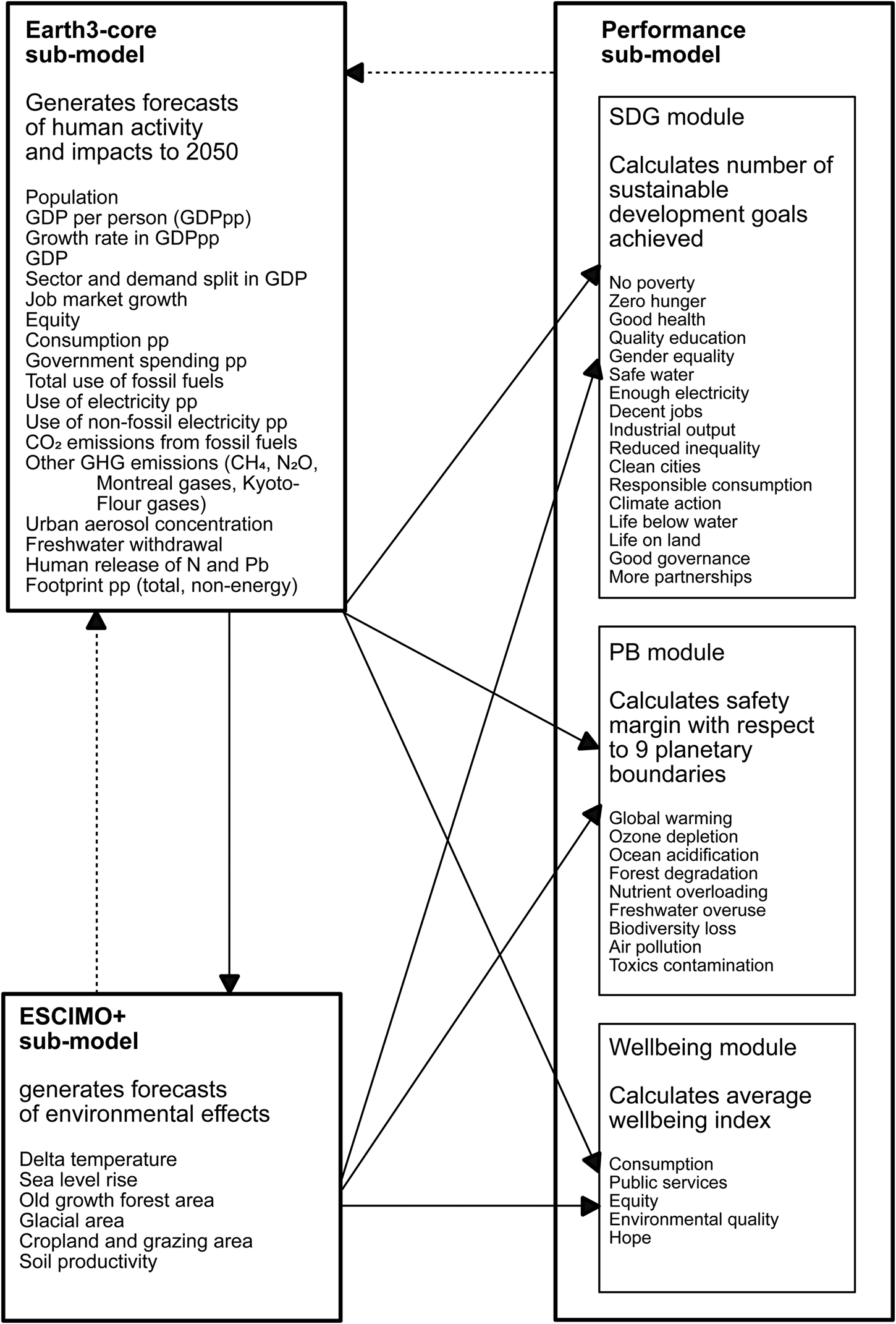
The detailed equations, parameter values and empirical basis of the Earth3 model system are described more fully in Goluke et al. (Reference Goluke, Randers, Collste and Stoknes2018) and Collste et al. (Reference Collste, Randers, Goluke, Stoknes, Cornell and Rockström2018). Earth3 consists of three interacting sub-models (Figure 1):
1. The socio-economic sub-model (Earth3-core) generates forecasts of the level of human activity to 2050, for seven world regions. Outputs include: population, GDP, income distribution, energy use, greenhouse gas release, and some other resource use and emissions.
2. The biophysical sub-model (ESCIMO-plus, Randers et al., Reference Randers, Goluke, Wenstøp and Wenstøp2016) calculates biophysical effects arising from human activity over the same time period. Outputs include: global warming, sea level rise, ocean acidity, forest area, extent of permafrost and glaciers, plus the productivity of biologically active land.
3. The performance sub-model (two modules, for SDGs and planetary boundaries) uses the outputs from the socio-economic and biophysical sub-models to calculate the development over time of three performance indicators: the number of the 17 SDGs achieved (by region); the safety margin (with respect to nine planetary boundaries); and an average Wellbeing Index (again by region).

Fig. 1. Overview of the Earth3 model system. Details in Goluke et al. (Reference Goluke, Randers, Collste and Stoknes2018). Dashed lines indicate where added feedbacks would convert Earth3 into a full system dynamics model.
2.2.1. The socio-economic sub-model
Earth3-core is a spreadsheet model written in Excel® 2016. The causal structure of Earth3-core is shown in Figure S1. Earth3-core utilizes high level relationships between SDG-relevant socio-economic variables and economic output expressed as Gross Domestic Product per person (GDPpp). In order to make comparisons between countries and over time, we use fixed (inflation adjusted) dollars, adjusted for purchasing power parity among nations, with 2011 as the base year. To give an example, we detail the relationship between births (CB in ‘per cent of the population per year’) and GDPpp. Figure 2a plots GDPpp on the horizontal axis as the independent variable and CB on the vertical axis as the dependent variable. Data are from 1960 to 2015, every fifth year, by region. Visual inspection confirms the central element of the demographic transition, namely falling birth rates for all regions and times where late-comers experience faster falling rates – when incomes rise. Figure 2b shows the same data but not by region. Using GNUplot to fit an exponential curve over the data in the form of
 $$f\lpar {\rm x} \rpar = a + b\cdot {\rm e}^{\left( {-\displaystyle{{{\rm GDPpp}} \over {\rm c}}} \right)}$$
gives a = 1.32, b = 2.97 and c = 5.22 with a root mean square of the residuals (RMSE) of 0.580.

Fig. 2. Examples of correlations used in Earth3-core (a–c) and the SDG performance module (d), based on historical data 1980–2015 for seven world regions. GDPpp is the independent variable in all cases. Panel a: births, as per cent of the population per year by region; b: births, globally; c: rate of change of GDPpp; d: fraction of population undernourished, as an indicator for SDG2. Details of correlations for all parameters are given in Goluke et al. (Reference Goluke, Randers, Collste and Stoknes2018) and Collste et al. (Reference Collste, Randers, Goluke, Stoknes, Cornell and Rockström2018).
We adjusted these parameters before using them in the model to better reflect demographic change. The dependent variable, births per population, contains the historical age pyramid of population in its historical data – it cannot do otherwise. Future age pyramids will likely be less pyramidal and more cylinder-like, with some nations even developing a top-heavy pyramid where older people outnumber younger people. We have adjusted a, which gives the minimum value for CB at high levels of GDPpp. We chose to set it at 0.8 to reflect age structures that become more dominated by old people in the future. We also rounded b to 3.0 and c to 5.0 giving a RMSE of 0.797 – statistically worse but causally better. (To be even more correct, we could replace our high-level formulation with a detailed age structure for each region and let that structure evolve causally dynamically – but then we would have left our intended path of low complexity modelling.) Finally, we forecast future values with this equation:
 $$CB_{\rm t} = CB_{{\rm t}-5}-\lpar {CB_{{\rm t}-5}-{\rm f}\lpar {\rm x} \rpar } \rpar \cdot \displaystyle{{{\rm dt}} \over {{\rm AT}}}$$
where dt is the solution interval, 5 years in our case, and AT is the adjustment time, which we set to 20 years. The causal meaning of this is that the crude birth rate approaches the value given by f(x) over a 20-year horizon. Equation [1] is a numerical approximation to the differential equation
 $$\displaystyle{{dCB} \over {dt}} = \displaystyle{{\lpar {CB-f\lpar x \rpar } \rpar } \over {AT}}$$
where
 $$f\lpar x \rpar = f\lpar {GDPpp} \rpar = 0.8 + 3.0\cdot e^{\left( {-\displaystyle{{GDPpp} \over {5.0}}} \right)}$$
and
 $$\displaystyle{{dGDPpp} \over {dt}} = f\lpar {GDPpp} \rpar $$
In this way we are able to replace very detailed mathematics with simple and transparent causal descriptions for many relationships in Earth3-core and the performance modules (Collste et al., Reference Collste, Randers, Goluke, Stoknes, Cornell and Rockström2018; Goluke et al., Reference Goluke, Randers, Collste and Stoknes2018). Figure 2c and 2d show other examples; the full list is shown in Tables S3 and S4.
We have been unable to endogenize some causal relations in a mathematical fashion. Inequality is one example, since it requires the dynamic development of income distributions as independent variables which we do not track in the Earth3-core spreadsheet. We therefore included a forecast for inequality exogenously, based on current trends (Alvaredo et al., Reference Alvaredo, Chancel, Piketty, Saez and Zucman2018). To leave the likely changes in inequality over the decades ahead in the business-as-usual scenario out would, in our judgement, be even less precise than to include it exogenously.
The forecast for the rate of change of GDPpp t as a function of GDPpp t-5 is based on the approach of Randers (Reference Randers2016) illustrated in Figure 2c.
In brief, values are calculated every five years through the following sequence:
1. Earth3-core simulates for each region the total output (GDP) per person through numerical integration, based on the historically observed correlation between the variables GDPpp and ‘rate of change in GDPpp’.
2. The size of the population is calculated based on values for birth and death rates that, in turn, depend on the value of GDPpp.
3. Total GDP is calculated as the product of population size and GDPpp.
4. Energy use (split between ‘use of electricity’ and ‘direct use of fossil fuels’ primarily for transport, heating and as raw material) is calculated as functions of GDPpp and population size.
5. CO2 emissions from energy use are calculated from the total use of fossil fuels and the fuel mix. The fuel mix is currently set exogenously in Earth3, as is the fraction of electricity from various sources, including renewable sources.
6. The use of resources and the release of other pollutants are calculated as functions of output and population and slowed by exogenous technological advance.
7. Income distribution, measured as the ‘share of national income to richest 10% of the population’, is exogenously determined based on historical trends.
8. Finally, the composition of GDP and of total demand is determined by the productivity level (i.e. GDPpp).
Whenever regional data exist, we estimated different parameter values for the different regions, thereby capturing the diversity of regional characteristics. Otherwise we estimated global averages. Where we discovered additional variation over time – for example indications of rapid technological advance – we included them as separate terms in the equations (see Table S3). Global activity levels are computed as the sum of the regional activity levels, weighted by population. Figure 3a and b shows some outputs from Earth3-core.

Fig. 3. Outputs from the socio-economic sub-model Earth3-core (a and b) and the biophysical model ESCIMO-plus (c and d) used to drive the Performance sub-model. Details in Goluke et al. (Reference Goluke, Randers, Collste and Stoknes2018). All outputs scaled from 0–1; output scale range given in key below each panel.
2.2.2. The biophysical sub-model
The biophysical sub-model ESCIMO-plus is a modified version of ESCIMO, a fully dynamic endogenous biophysical system model of low complexity (Randers et al., Reference Randers, Goluke, Wenstøp and Wenstøp2016), written in Vensim®. The modifications allow it to be driven by Earth3-core greenhouse gas emission scenarios. In contrast to the regionalized Earth3-core, ESCIMO-plus generates global average values for its variables when driven by outputs from Earth3-core. The causal structure of ESCIMO-plus is shown in Figure S2.
ESCIMO-plus dynamically and endogenously keeps track of carbon flows and stocks in the global ecosystem, of global heat flows and stocks, and of the areal extent and productivity of varying land types. ESCIMO-plus ensures conservation of carbon, heat, land area and biomes in model simulations, assuring consistency among scenarios. The current model does not conserve water, which appears in different forms in ESCIMO-plus – as ocean water, fresh water, ice and snow, vapour, and low and high clouds. Sensitivity analysis shows (Randers et al., Reference Randers, Goluke, Wenstøp and Wenstøp2016) that the biophysical sub-model is generally robust, except minor changes in the treatment of clouds and water vapour lead to major change in the model output, particularly in the long run (i.e. after 2050). These physical processes are persistently challenging issues in much more comprehensive modelling of Earth's dynamics (Boucher et al., Reference Boucher, Randall, Artaxo, Bretherton, Feingold, Forster, Wyant and Stocker2013; Flato et al., Reference Flato, Marotzke, Abiodun, Braconnot, Chou, Collins, Zhang and Stocker2013). We have stuck to our simple formulations, in the hope of finding less sensitive, but still tractable, solutions in future work.
Outputs from ESCIMO-plus include global average temperature rise, average sea level rise, ocean acidity, the extent of different land types, and others of relevance to planetary boundaries. Figure 3c and d shows some examples. The output from ESCIMO for given drivers has been compared with the output of other much more complex earth system models, including the models of the Climate Model Intercomparison Project (CMIP, 2016). Although ESCIMO is very simple to use, it generates similar results to the bigger models when subject to the same drivers (Randers et al., Reference Randers, Goluke, Wenstøp and Wenstøp2016).
2.2.3. The performance sub-model
The performance sub-model consists of two parts: one module measures the performance of achieving the SDGs and the other measures how well humanity stays within the planetary boundaries while trying to achieve the SDGs.
The outputs of Earth3-core and ESCIMO-plus are used as inputs in the performance sub-model, to generate three performance indicators relating to global sustainability objectives: the number of SDGs achieved; the global ‘safety margin’ calculated as the number of planetary boundaries kept within their low-risk zone; and the average wellbeing of the typical citizen in the region of interest, based on five components. Together, these performance indicators (Figure 4) facilitate comparison of alternative pathways as they evolve over time. All three indicators are calculated every fifth year, for every region except in cases where we only have global data.

Fig. 4. Outputs from the Performance sub-model 1980–2050.
2.3. The SDG success rate: the number of 17 SDGs achieved
This performance indicator measures the extent to which the SDGs are achieved in the model system, on an overall scale from 0 (no achievement at all) to 17 (full achievement of all goals). For each SDG, we specify one modellable indicator and define two threshold values for each indicator (Table 1), defining green, amber and red zones in the pathway plots. Green means that the SDG in question has been reached, red means it has not been reached. For example, for SDG1, the green zone denotes less than 2% of the population living below $1.90/day and is assigned a score of 1. The red zone is more than 13% of the population living below $1.90/day, assigned a score of 0. The zone between green and red we call amber and assign a score of 0.5.
Table 1. The 17 Sustainable Development Goals and 9 planetary boundaries in Earth3. Details in Table S1 in supplementary materials. GDP and Government spending are in 2011 PPP US$.

The number of 17 SDGs achieved is the sum of achievement scores for all 17 SDGs, calculated per region (Figure 4a). By summing the regional results weighted by population, we obtain an aggregate measure of the global average number of SDGs achieved (Figure 4b). In doing this, we weight each SDG equally in line with Agenda 2030, where the SDGs are ‘integrated and indivisible’. It is of course fully possible to choose different weights for different SDGs, by making minor changes in the spreadsheets in the SDG module of the performance sub-model.
2.4. The safe operating space for humanity: the global safety margin with respect to 9 PBs
This performance indicator measures the intensity (in the model system) of human pressure on Earth's life-supporting systems relative to our estimate of the planetary boundaries (termed PBs in the model system). The global safety margin is given on a scale from 9 for no pressure on any of nine planetary boundaries to 0 when human impacts have pushed beyond the safe operating space for all planetary boundaries. As for SDG achievement, we define two threshold values for the pressure on each planetary boundary (Table 1), marking a green low-risk zone (safety margin score 1), an amber medium-risk zone (score 0.5) and a high-risk red zone (score 0). For example, for PB1 – global warming – the green zone is an increase of less than 1°C over pre-industrial global average temperature, with a score of 1. The red zone is a temperature increase of 2°C or more, scoring 0. The global safety margin with respect to 9 PBs is the sum of the safety margin scores for all planetary boundaries, assessed globally. The result can be seen already by splitting the SDGs into 14 socio-economic and 3 environmental ones (Figure 4c; for PBs see Figure S3a).
3. Average Wellbeing Index
Reaching 17 SDGs within 9 PBs over time is a lot of indicators to track. Merely enumerating them one by one is possible, but drowns any message, even for one country (European Commission, 2019). Others have flagged the need for a transparent aggregated index but have not progressed beyond theoretical considerations of what such an index should accomplish (Chandrakumar & McLaren, Reference Chandrakumar, McLaren, Benetto, Gericke and Guiton2018; Clift et al., Reference Clift, Sim, King, Chenoweth, Christie, Clavreul and Murphy2017; Moyer & Bohl, Reference Moyer and Bohl2019; O'Neill et al., Reference O'Neill, Kriegler, Riahi, Ebi, Hallegatte, Carter and van Vuuren2014, Reference O'Neill, Fanning, Lamb and Steinberger2018; Riahi et al., Reference Riahi, van Vuuren, Kriegler, Edmonds, O'Neill, Fujimori and Tavoni2017; Wackernagel et al., Reference Wackernagel, Hanscom and Lin2017).
We suggest a new indicator that is suited to the task of summarizing the status of humanity's effort to achieve 17 SDGs within 9 PBs, and that can be useful as a high-level communication device. The average Wellbeing Index is intended to measure the wellbeing of a typical inhabitant in a region. It is defined as the arithmetic mean of the scores on five indicators of personal wellbeing (Table S2). The five indicators and their ‘satisfactory level’ are as follows:
1. private consumption of goods and services (>10.000 2011 PPP US$/person-year);
2. supply of public services available to each person (>1.500 2011 PPP US$/person-year);
3. equity in income distribution, defined as the share of national income going to the richest 10 per cent (< 40%);
4. quality of the biophysical environment, defined as fine particulate matter concentration in urban aerosol (< 10 µg PM2.5/m3); and
5. hope for a better future, defined as the recent rise in global temperature (< 0.05°C warming in 20 years).
These five components are meant to illustrate the approach. Other choices are fully possible and defensible, but they need to span the domain of reaching all SDGs within PBs and engage with the dynamics of sustainable development. Well-established indicators, like the Human Development Index, Ecological Footprint and even GDP per person, do not suffice because they do not cover the entire domain.
Each indicator is measured relative to its satisfactory level. Therefore, the average Wellbeing Index will equal 1 when all indicators are at the satisfactory level, and 0 when there is no satisfaction at all of any of the components. Figure 4d shows, by region, the result in the business-as-usual scenario.
We calculate the global average wellbeing as the sum of the Wellbeing Indices for all regions weighted by their population. This provides a single time series for the business-as-usual scenario (Figure 4d), and for any other scenario (Figure S3b), making it simpler to compare different scenarios.
4. Results: Business-as-usual in Earth3
In this paper we discuss one scenario produced with the Earth3 model system. We run ‘business-as-usual’ from 2018 to 2050 to describe the consequences on the level of human activity and the resulting biophysical effects. We have made other scenarios of accelerated economic growth, a stronger focus on SDGs and sustainability transformation (Randers et al., Reference Randers, Rockström, Stoknes, Goluke, Collste and Cornell2018). For each of these scenarios, the output from Earth3 constitutes a consistent, quantitative backbone of the broad developments towards 2050.
Business-as-usual is the baseline run of Earth3. It is made to match recent history and provides a picture of what is likely to happen if there are no extraordinary changes in human behaviour. We use parameters that track general trends in historical data from 1980 to 2015 to project regional and world development to 2050. The chosen parameters reflect our overall assumption in this scenario that the decision makers of the world will continue to perceive and respond to emerging problems in the conventional manner, with the gradual institutional development seen in the past few decades that we believe is likely to extend to the decades ahead.
Earth3-core tells the following story in the business-as-usual scenario:
Towards 2050, population growth slows down. In most regions population numbers stagnate, and in some they decline, with exception of the poorest regions, where population growth continues. Economic production (GDP) continues to grow everywhere, at high rates in China and many emerging economies, but at low rates in the rich regions, with stagnation in some cases. Per capita incomes continue up, but inequity – measured as the share of national income accruing to the richest 10% of the population – continues to rise in most regions, especially in the free market economies. (Figure 3a)
Energy use increases, but electricity use grows faster than fossil fuel use, which peaks around 2040. Electricity increasingly comes from renewable sources, and fossil fuel use for electricity generation peaks and declines in the 2030s. In the 2030s, greenhouse gas emissions also peak, because of increasing energy efficiency, the shift to wind and solar power, and the phasing out of other Kyoto and Montreal gases. The use of nitrogen and fresh water, as well as the release of lead, continue to rise, but at slowing rates. (Figure 3b)
ESCIMO-plus tells the following story about the resulting biophysical effects to 2050:
Global warming continues and reaches + 2°C already by 2050. Sea level rises by ~30 cm, the oceans become more acidic, on-land glaciers and permafrost area shrink. Old-growth forest area – both tropical and Northern – declines by another 20%. The fertilization effect of CO2 on soil productivity is increasingly counteracted by negative effects of higher temperatures and more variable precipitation. On the positive side, the concentrations of greenhouse gases decline and the amount of unused biocapacity stays above a lower threshold. (Figure 3c and d)
In summary, in business-as-usual scenario from 2018 to 2050, human societies become richer, in the sense that people live in countries with higher GDP per person, but they live in more unequal societies and in an environment that is increasingly damaged by human activity.
To what extent will the SDGs be achieved in this business-as-usual scenario? Figure 4a shows the number of SDGs achieved by region from 1980 to 2018. (Figure S4 shows the result for each SDG, by region.) Figure 4b shows the global average sustainable development progress since 1992. Figure 4c distinguishes between socio-economic and environmental SDGs and suggests that humanity has chosen to try to meet the former at the expense of the latter. For the environmental goals 13, 14 and 15, the situation deteriorates (Figure 4c-lower lines), as human pressures on climate, water and land continue to rise. In rich regions, the impact of the declining environmental SDGs on overall SDGs achievement leads to a general decline over coming decades. Going forward, global society (in the model system) achieves 10.5 of the 17 SDGs by 2030 and 11.5 by 2050 – up from 9 in 2015.
Figure S5 shows the resulting pressure on the planetary boundaries under business-as-usual. For most, the indicators move towards the higher-risk red zone. The exceptions to this problematic trend are ozone depletion, as releases of Montreal gases continue to decline, and air pollution, where the population affected by anthropogenic haze declines from 2020 onwards.
Again, the aggregated global measure gives a less noisy picture. Figure S3a-blue line shows a steadily shrinking global safety margin, from 8 in 1980, to 4.5 in 2018 and 2030, and 3.5 in 2050. In other words, by mid-century humanity (in the model system) has transgressed eight of the nine planetary boundaries and is deeply into the high-risk red zone for four of them.
Finally, to illustrate how humanity deals with reaching socio-economic and environmental SDGs and staying within planetary boundaries we look at how average wellbeing evolves under business-as-usual. Figure S3b shows that global average wellbeing remained largely constant from 1980 to 2020, because economic growth was insufficient to compensate for the combined effect of increasing inequity, increasing pollution levels, and increasing concern about dangerous climate change. Wellbeing rises towards 2050 in the business-as-usual scenario (blue line), because more people become better off: increased consumption counterbalances the negative effects of inequity, pollution and climate change. In the rich world, average wellbeing grew to 2020, but progress slows going forward, because the dis-amenities of inequity, pollution and despair grow faster than consumption and public service supply. In other regions, wellbeing rises from 2020, albeit from lower levels. In China, average wellbeing reaches Western levels at the end of the simulation period (Figure 4d).
This assessment depends on the weights chosen for the five components of the average Wellbeing Index. We weighted them equally as a demonstration of the Earth3 system. It would be simple to defend other weightings, and users of Earth3 are encouraged to do so in their exploration of policy ideas.
In sum, the business-as-usual scenario does lead to a rise in the number of SDGs achieved by 2030, and to a rise in average wellbeing globally. But there is little improvement on the SDGs to 2050, and at the same time the human pressure on the environment grows, eroding the global safety margin relative to the planetary boundaries.
5. Sensitivity analysis
For those used to equilibrium models and seeing the world in equilibrium terms, it is important to note that we see the world as a system away from equilibrium, with causal assumptions and parameter values selected in line with this view. We work in the system dynamics tradition of modelling and model validation (Barlas, Reference Barlas1996). The validation of a system dynamics model is contingent upon the model's purpose and typically includes not only behavioural pattern tests, as typically used in statistical models, but also structure tests and structure-oriented behaviour tests. An overall check of model plausibility was conducted by comparing the output of Earth3-core with two major global modelling efforts: DNV-GL's Energy Transition Outlook 2018 (DNV-GL, 2018) and IIASA's global population model (Lutz et al., Reference Lutz, Goujon, Samir, Stonawski and Stilianakis2018). We found no discrepancies that warranted model adjustment.
All models are subject to uncertainties. Earth3 is work in progress, so we remain uncertain about the level of precision in our conclusions due to the sensitivity in the numerous inputs used to generate them. If it were a fully endogenized model, Monte Carlo sensitivity analysis would be possible and appropriate. In order to get a better feel for Earth3 as it currently stands, we performed a simple sensitivity analysis focused on GDPpp, because it is such a central variable in the model. We changed our assumption about economic growth in the following manner:
Our formula for the rate of change of GDPpp is
 $$ \eqalign{&{\rm RoC}\lpar {{\rm GDPp}{\rm p}_{\rm t}} \rpar = \Big( {{\rm RoC}\lpar {{\rm GDPp}{\rm p}_{{\rm t}-5}} \rpar -\lpar {{\rm RoC}\lpar {{\rm GDPp}{\rm p}_{{\rm t}-5}} \rpar }}\cr& {{- {\rm a}\cdot {\rm e}^{\lpar {-{\rm b}\cdot {\rm GDPp}{\rm p}_{{\rm t}-5}} \rpar }-{\rm c}\cdot {\rm e}^{\lpar {-{\rm d}\cdot {\rm GDPp}{\rm p}_{{\rm t}-5}} \rpar }} \rpar \cdot \displaystyle{{{\rm dt}} \over {{\rm AT}}}} \Big)$$
where a = 9.0, b = 0.07, c = 6.0, d = 0.3, dt = 5 and AT = 20 (using logic like the crude birth rate formulation detailed above). To run the sensitivity test, we add an additive term of either +1 percentage point (accelerated economic growth) or −1 percentage point (slower economic growth).
The resulting impact on world SDGs and PBs is shown in Figures 4b, 4c and S3a. In 2050, 11.9 SDGs are reached for both accelerated and slower growth, as opposed to 11.5 under business-as-usual. However, the trajectory towards 2050 is better (i.e. more SDGs reached) for accelerated growth and much better for slower growth. Thus, adding or subtracting 1 percentage point to our formula above results in a 3.5% increase in global SDGs met by 2050. For PBs, both business-as-usual and accelerated growth end up with 3.5 boundaries met in 2050 and with 5 boundaries met for slower growth. Here, slowing growth by 1 percentage point results in a 35% increase in staying within PBs. This high sensitivity points to the need to endogenize the model.
Still, our main finding holds, that humanity will not be able to achieve the social and environmental SDGs, within planetary boundaries – without extraordinary action.
6. Discussion and conclusions
In the Earth3 model system, humanity does not achieve the SDGs within planetary boundaries by 2030, nor even by 2050 in the business-as-usual scenario. It also points out that whatever achievement humanity reaches on the socio-economic SDGs it pays a heavy price on the environmental SDGs, raising the spectre that Griggs’ warning of 2013 (Griggs et al., Reference Griggs, Stafford-Smith, Gaffney, Rockström, Öhman, Shyamsundar and Noble2013) might indeed come true. A sensitivity analysis shows little effect on this main conclusion from changes in the rate of change in GDP per person. But as in all modelling studies, our conclusions depend on the assumptions made.
Earth3 in its current form should be seen as a starting point – a proof of concept – for further elaboration. The low complexity of the model structure makes our principal assumptions transparent, but in some cases other assumptions may be equally plausible and would lead to different conclusions. Important examples are our choice of indicators for the individual SDGs and PBs, the choice of thresholds, and the choices of functional form, satisfactory levels and weighting in the Wellbeing Index. Thus, Earth3 is not a sustainability forecaster, but a ‘what-if’ calculator – which, in the end, all models are, even the high complexity IAMs and comprehensive earth system models that currently inform much global policy. When reality differs from the assumptions made, the more transparent and flexible the model, the more useful it can be in re-diagnosing the issues.
In its current formulation, Earth3 has no feedback from the biophysical sub-model to the socio-economic model. Examples where this matters are our exogenous treatment of inequity and near-exogenous treatment of forest cut. In our view, this limitation matters much more in the long run (i.e. after 2050), because history indicates that humanity responds slowly to changes in the global environment.
Methodologically, the Earth3 study shows that it is possible to build a global system model and use it to analyse future achievement of all SDGs within PBs. But despite its usefulness as an exploratory tool, Earth3 is far from perfect. New generations of integrated World-Earth models are needed to test and sharpen our conclusions, and to study the feasibility and consequences of transformational change. Much work remains to achieve a fully causally endogenous global model system that can provide better assessments of the consequences of alternative global policy sets on the achievement of the 17 SDGs and the evolution of the safety margin relative to planetary constraints. We plan to continue the work of developing and using a transparent low complexity dynamic model, cheap to run by everyone, and hope to inspire others to do likewise.
Supplementary material
To view supplementary material for this article, please visit https://doi.org/10.1017/sus.2019.22
Acknowledgements
We thank the Shanghai Academy of Social Sciences in Shanghai and the KR Foundation in Copenhagen for crucial moral and financial support to earlier stages of this project. We also thank two anonymous reviewers for valuable comments.
Author contributions
JRo conceived the study of SDGs within PBs. JRa designed the approach and built the central models in close cooperation with UG. DC gathered data on SDGs and PBs and contributed to the SDG module. PES devised the scenario perspective and contributed to SDG and PB modules, JD and SC positioned the study in the sustainability science literature. JRa wrote the paper, greatly assisted by SC.
Financial support
The work was made possible by a grant from the Global Challenges Foundation in Stockholm. DC thanks the European Union's Horizon 2020 research and innovation programme for support under the Marie Sklodowska-Curie Grant Agreement No. 675153 (ITN JD AdaptEconII). SC acknowledges partial funding from the European Research Council through JRo's Advanced Grant Earth Resilience in the Anthropocene.
Conflict of interest
None.
Ethical standards
Both the paper and the Earth3 model system are the original work of the authors.


 Open access