


1. Introduction
The availability of dense single-nucleotide polymorphism (SNP) arrays has considerably changed the landscape of dairy cattle selection worldwide. With such chips, it is now possible to retrieve information about quantitative trait locus (QTL) all over the genome. Genomic estimated breeding values (GEBV), which correspond to a combination of the sum of the effects of genetic markers (direct genomic value (DGV)) and estimated breeding value (EBV), can be used instead of the classical pedigree-based genetic evaluations in selection programmes. Meuwissen et al. (Reference Meuwissen, Hayes and Goddard2001) envisioned the consequences on the estimation of breeding values of a high-density marker map covering the whole genome (see also Haley & Visscher, Reference Haley and Visscher1998; Andersson & Georges, Reference Andersson and Georges2004). Through simulations, they showed that the use of GEBV can greatly improve accuracy of genetic evaluation of animals with no recorded performances hence leading to higher genetic gain, particularly by shortening generation intervals in dairy cattle. In dairy cattle, the use of GEBV is a promising alternative to the long and costly progeny test. Since 2007, the potential interest of genomic selection in dairy cattle has been clearly demonstrated in terms of accuracy of breeding values (Van Raden et al., Reference Van Raden, Van Tassell, Wiggans, Sonstegard, Schnabel and Taylor2009; Habier et al., Reference Habier, Fernando, Kizilkaya and Garrick2011) and in terms of design of breeding programmes (Goddard & Hayes, Reference Goddard and Hayes2007; Wensch-Dorendorf et al., Reference Wensch-Dorendorf, Yin, Swalve and König2011). Recently, several countries (Australia, France, Germany, the Netherlands, New Zealand, USA and others) implemented genomic selection for their national evaluations (Hayes et al., Reference Hayes, Bowman, Chamberlain and Goddard2009; Van Raden et al., Reference Van Raden, Van Tassell, Wiggans, Sonstegard, Schnabel and Taylor2009; Boichard et al., Reference Boichard, Guillaume, Baur, Croiseau, Rossignol and Boscher2010; Harris & Johnson, Reference Harris and Johnson2010; Liu et al., Reference Liu, Seefried, Reinhardt, Thaller and Reents2010).
Numerous methods have been proposed to perform genomic evaluations with variable resulting accuracy depending on the underlying genetic assumptions, on the trait, breed and reference population size. For instance, Habier et al. (Reference Habier, Fernando, Kizilkaya and Garrick2010a) tested a large panel of Bayesian approaches on a data set from the Holstein breed and even though Bayes A appeared to be a nearly optimal choice in their study, they recommended determining the best method for each quantitative trait separately. Indeed, in another study on Australian Holstein Friesian dairy cattle, Bayes A provided the lowest correlation between predicted GEBV and breeding values among the set of tested methods (Verbyla et al., Reference Verbyla, Hayes, Bowman and Goddard2009). On French data that Legarra et al. (Reference Legarra, Robert-Granié, Croiseau, Guillaume and Fritz2011) conducted for production traits, better predictions were obtained for Bayesian LASSO than for genomic BLUP (gBLUP). For other traits like fertility, it was shown that gBLUP performed slightly better than Bayesian LASSO (Hayes et al., Reference Hayes, Bowman, Chamberlain and Goddard2009; Van Raden et al., Reference Van Raden, Van Tassell, Wiggans, Sonstegard, Schnabel and Taylor2009).
Hence, it is still difficult to rank the large panel of available genomic evaluation methods according to their accuracy.
In a genomic evaluation procedure where the complete set of SNP is used, the statistical challenge is to evaluate effects attached to each of the available SNPs. In a context where the number of SNPs (p) is much higher than the number of bulls (n), this may lead to a poor estimation of the SNP effects even though the sum of genotypes time effects may be adequate on this reference population. In a routine evaluation with new animals, the best way to be confident in DGV or GEBV is to attach an effect to SNP in linkage disequilibrium with a QTL which reflects the effect of the QTL and an effect regressed towards zero to the others.
An alternative is to use approaches that have been developed especially to solve the p>>n problem. This is the case of variable selection methods and, among them, we focused on the Elastic-Net (EN) algorithm (Zou & Hastie, Reference Zou and Hastie2005) and we chose to compare it to gBLUP, which is currently the most used approach in practice. Secondly, a two-step approach was tested by adding an initial preparation step consisting of an SNP pre-selection based on results from a QTL detection analysis. The second step implements gBLUP or EN on this preselected set of SNP with the hope that individual estimates of effects of the retuned SNP would be more accurate. To compare benefits and drawbacks of these situations, a pedigree-based BLUP was used as the reference.
2. Materials and methods
2.1 Data
The data sets consisted of 1172 Montbéliarde, 1218 Normande and 3940 Holstein bulls, which were all progeny tested and genotyped with the Illumina Bovine SNP50 BeadChip®. With a minimum minor allele frequency of 3%, 38 460 SNPs were retained for the Montbéliarde breed, 38 534 SNPs for the Normande breed and 39 738 SNPs for the Holstein breed. Mendelian segregation was checked. The SNP pre-selection chosen in this study uses a QTL detection method based on haplotypes which requires phased data. To infer missing genotypes and phases, DualPHASE software was used (Druet & Georges, Reference Druet and Georges2009).
The data set was divided into a training data set to derive prediction equations and a validation data set where predictions were compared with observed phenotypes. Table 1 shows the size of training and validation data sets for the three breeds. To define the training and validation data sets, a cut-off date for the bulls’ birth date was introduced so that 25% of the youngest genotyped bulls were included in the validation dataset. Bulls without genotyped sire in the training dataset were excluded. Animals from the training data set were born before June 2002, while animals from the validation data set were born between June 2002 and 2004. This cross-validation design corresponds to the one used in studies of the EuroGenomics Consortium (Lund et al., Reference Lund, de Roos, de Vries, Druet, Ducrocq and Fritz2010).
Table 1. Number of animals genotyped per data set for the three breeds studied

Phenotypes used for this study were daughter yield deviations (DYD) corresponding to the average performance of a sire's daughters, adjusted for fixed and non-genetic random effects and for the additive genetic value of their dam (Mrode & Swanson, Reference Mrode and Swanson2004). To account for the varying accuracy of the DYD, they were weighted by their error variance, which is proportional to the sire's effective daughters’ contribution (EDC) (Fikse & Banos, Reference Fikse and Banos2001). DYD were included in the analysis if EDC exceeded 20.
For the three breeds, 25 traits were available: five production traits, two conception rate traits, 16 morphological traits, somatic cell counts and milking speed. Initially, only six traits were chosen to compare the different approaches and for fine tuning of different parameters. These six traits were the five production traits (Milk yield, Fat yield, Fat content, Protein yield and Protein content) and cow conception rate (Boichard & Manfredi, Reference Boichard and Manfredi1994). Mean results over the 25 traits will also be shown.
(ii) Methods
The first method used was gBLUP (Van Raden et al., Reference Van Raden2008) which uses the genomic relationship matrix, G (Habier et al., Reference Habier, Fernando and Dekkers2007; Van Raden, Reference Van Raden2008), instead of the pedigree-based relationship matrix
where m corresponds to the number of loci considered, pi is the frequency of an allele of the locus i and Z is the incidence matrix of SNP (genotype scores) on individuals, coded as in Van Raden (Reference Van Raden2008) . The model is therefore: y=Xb+g+e, where g is a vector of breeding values whose covariance matrix is described by Gσu2, where σ u 2 is the polygenic variance.
Van Raden (Reference Van Raden2008) and Goddard (Reference Goddard2009) showed that this model is equivalent to a mixed model fitting the effect of the genotype score of each SNP, all SNPs having a priori the same variance equal to ![]() , where σ
u
2 is the polygenic variance used in regular genetic evaluation and pi
is the frequency of an allele of the locus i (Gianola et al., Reference Gianola, de los Campos, Hill, Manfredi and Fernando2009).
, where σ
u
2 is the polygenic variance used in regular genetic evaluation and pi
is the frequency of an allele of the locus i (Gianola et al., Reference Gianola, de los Campos, Hill, Manfredi and Fernando2009).
The EN algorithm (Zou & Hastie, Reference Zou and Hastie2005; Croiseau et al., Reference Croiseau, Guillaume, Fritz and Ducrocq2009) corresponds to a combination of the ridge regression (RR) and LASSO procedures. The difference between RR ![]() and LASSO
and LASSO ![]() estimates lies in the form of the penalty term. In both equations, β is the vector of SNP effects β
j
, yi
is the phenotype of animal i and xi is its vector of genotypes. The λ parameter corresponds to the intensity of the penalty. In the EN algorithm, a second parameter α, taking a value in [0, 1] is used to weight the RR and LASSO penalties.
estimates lies in the form of the penalty term. In both equations, β is the vector of SNP effects β
j
, yi
is the phenotype of animal i and xi is its vector of genotypes. The λ parameter corresponds to the intensity of the penalty. In the EN algorithm, a second parameter α, taking a value in [0, 1] is used to weight the RR and LASSO penalties.

With α=1, a LASSO model is defined, whereas with α=0, a full RR model is chosen. Zou & Hastie (Reference Zou and Hastie2003, Reference Zou and Hastie2005) showed that in the presence of correlated explanatory variables (e.g. effects corresponding to SNP in linkage disequilibrium in our case), RR retains all predictors and their corresponding coefficients tend to be equal and no variable selection is performed. On the other hand, LASSO retains only one predictor and removes the others (Zou & Hastie, Reference Zou and Hastie2003, Reference Zou and Hastie2005). Hence, by including RR and LASSO as extreme cases, the EN algorithm provides a more flexible tool.
In this study, EN procedures were used using an R package named ‘glmnet’ (http://cran.r-project.org/web/packages/glmnet/index.html) implemented by Friedman et al. (Reference Friedman, Hastie and Tibshirani2008) . They proposed a fast implementation of EN using cyclical coordinate descent, computed along a regularization path.
(iii) Pre-selection of the SNP
For most traits, not all SNPs on the SNP chip are likely to be close to a QTL. In other words, the assumption that effects attached to each of the SNPs are non null is unrealistic. Consequently, our conjecture is that whatever the genomic evaluation method used, a pre-selection of the SNP with an attached non-null effect may help to improve the quality of genomic prediction. This was tested in the situation where pre-selection is based on QTL detection. QTL detection was performed using a combined linkage disequilibrium and linkage analysis (LDLA) (Meuwissen & Goddard, Reference Meuwissen and Goddard2001; Druet et al., Reference Druet, Fritz, Boussaha, Ben-Jemaa, Guillaume and Derbala2008). First, the existence of a single QTL was tested in the training data set at all positions along the chromosomes defined by haplotypes of six SNPs, with a sliding window of two SNPs. From this LDLA, a value of the likelihood ratio test (LRT) was obtained for each haplotype. Positions where a potential QTL is located were defined as haplotypes each time an LRT peak higher than a threshold value of 3 or 5 was found. These values were quite arbitrary at this stage and low enough to catch any potential QTL that can be identified through this analysis. An LRT peak was defined as the position where the highest LRT value was found within a window of 25 or 50 SNP upstream and downstream of the current haplotype.
Then, the 50 SNPs around each detected LRT peak (±25) were included in a pre-selected set of SNPs used for genomic evaluation using either a gBLUP or EN approach. The choice of the number of SNPs to retain was based on a preliminary study where this value of 50 gave the best results (data not shown).
(iv) Quality assessment of the genomic prediction
To measure the quality of prediction equations (derived from the training set), the equations were applied to the animals of the validation data set to get DGVs. Then, the weighted correlation between DGV and observed DYD was computed using EDC as weights. The weighted Pearson product moment correlation coefficient is calculated as (Peers, Reference Peers1996):

where ![]() ,
, ![]() and wi
is the EDC weight of yi
.
and wi
is the EDC weight of yi
.
The aim was to measure the accuracy of the different methods to predict DYD using genomic information (DGV). Since GEBV combine the information available from DGV and EBV, it is not possible to know if an observed gain in accuracy is due to the prediction equation or to a good combination of DGV and EBV. This is why the correlation between DGV and observed DYD was preferred in this study (see e.g. Guillaume et al., Reference Guillaume, Fritz, Boichard and Druet2008).
(v) Parameters used for the different methods
For the pedigree-based BLUP, genetic parameters were estimated using an Average Information-Restricted Expectation Maximization Likelihood (AI-REML) approach (Jensen et al., Reference Jensen, Mantysaari, Madsen and Thompson1996). For the LDLA, it is necessary to incorporate Identical by Descent (IBD) matrices among QTL allelic effects. Software of Misztal et al. (Reference Misztal, Tsuruta, Strabel, Auvray, Druet and Lee2002) was modified accordingly. Heritability estimates used in pedigree-based BLUP and gBLUP were those used in routine genetic evaluations.
For EN, values for the α and λ penalization parameters needed to be chosen and there is currently no way to predict which range of values is the most appropriate for each parameter. Consequently, a large range of combinations of α and λ was tested by grid search to find the optimal values. The search aimed at finding the maximum correlation between DGV and observed DYD in the validation data set. The validation data set is consequently used to identify the optimal set of parameters. This can be an advantage in comparison with other methods with respect to the accuracy of GEBV if this set of parameters is specific to this training and validation data sets. However, by looking at reference populations of increasing sizes, we found that these parameters were breed- and trait-specific with a rather large range of combinations giving similar results (data not shown). The EN approach appears robust to moderate departures from the optimal combination of parameters. To define the optimal α parameter, a dichotomous search was performed on the [0, 1] interval. Initially, α values of 0, 1 and 0·5 were tested. If α=0 provided the best correlation, at the second iteration, the interval was reduced to [0, 0·5]. If the best correlation was found with α=1, the new interval was [0·5, 1]. If the best correlation was found with α=0·5, the new interval was [0·25, 0·75]. We applied this method until the difference between two tested α was lower than 0·02. The dichotomous approach requires a unimodal distribution for these correlations which is not guaranteed. Nevertheless, after testing a large panel of α values for some traits (data not shown), this unimodal distribution seems to be the rule.
For each α, 500 values of the penalty intensity λ were tested in the interval [0–max(β)], where max(β) corresponds to the absolute value of the highest estimate when no penalization is applied.
This research of optimal values for α and λ was performed separately for the pre-selected and the full data sets. The search for the optimal α parameter is the most time-consuming step of the glmnet package and takes around 2 CPU minutes in Holstein for each tested α.
3. Results
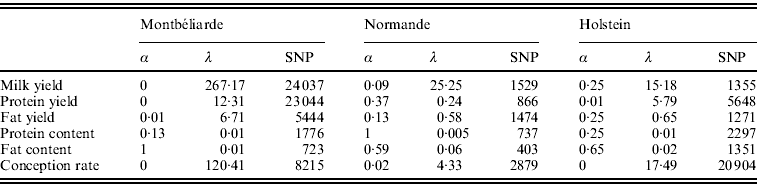
Table 2 shows the optimal set of EN parameters for the six traits initially studied. Depending on the trait and breed, the optimal set of parameters differed. For instance, a complete RR approach gave the best results for Milk and Protein yield in the Montbéliarde breed, while optimal α values of 0·25 for Milk yield in Holstein and of 0·37 for Protein yield in Normande were found, which correspond to a general EN model. Moreover, there was a strong impact of both α and λ on the number of SNPs included in the regression model. When α is near a complete LASSO procedure (α=1), there were many fewer SNPs retained compared with a complete RR procedure (α=0). Also, for a given a, high values of λ led to a high intensity of penalization and consequently to a lower number of SNP (results not shown).
Table 2. Optimal α and λ parameters and corresponding number of SNPs with non-null effect for the six traits studied and for the three breeds using the EN procedure on the complete set of SNPs
In the second analysis, the SNP pre-selection based on QTL detection was performed. As indicated before, this SNP pre-selection relied on two criteria: a given LRT threshold and a given window size. Table 3 reports the effect of both criteria on the number of LRT peaks identified in the case of milk yield.
Table 3. Number of LRT peaks identified for milk yield as a function of LRT threshold and window size in the Montbéliarde, Normande and Holstein breeds
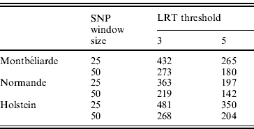
Table 4 presents for the three breeds the results obtained with the classical pedigree-based BLUP and the two genomic selection methods (gBLUP and EN) when either the whole set of SNP which passed the quality control was used or after a pre-selection of the SNP based on the LDLA approach.
Table 4. Weighted correlation between DGV and observed DYD for the three breeds obtained using pedigree-based BLUP, gBLUP and EN on the complete set of SNP (54 K) or after a pre-selection of the SNP (PS)

All genomic methods improved the correlation between DGV and observed DYD compared with pedigree-based BLUP and the genetic architecture of the trait seemed to play an important role on the gain in correlation: for traits where some QTLs explain a large part of the variance, such as protein content and fat content (where DGAT1 gene is present), a mean gain in correlation over the three breeds of +0·22 and +0·23, respectively, was observed. In contrast, when the trait background appears to be polygenic with many QTLs explaining only a small part of the variance each, as for conception rate, the observed mean gain in correlation was more limited (+0·06). Between the two genomic approaches, EN gave better results with a mean gain (compared with pedigree-based BLUP) over the six traits of 0·15, 0·13 and 0·20 for Montbéliarde, Normande and Holstein, respectively, compared with 0·12, 0·08 and 0·18 with gBLUP.
When an SNP pre-selection was applied, the gain in correlation using gBLUP and EN was very similar to the one observed using the complete set of SNP. Again, among the two different genomic approaches, the best results were obtained with EN. Compared with the pedigree-based BLUP, the mean gains over the six traits were 0·14, 0·15 and 0·20 for Montbéliarde, Normande and Holstein, respectively, compared with 0·12, 0·11 and 0·18 with gBLUP.
Table 5 shows the slope of the regression of observed DYD on DGV for Holstein. A value close to 1 is expected. In dairy cattle, genomic evaluations are validated by Interbull if the slope of regression is included between 0·8 and 1·2 (Interbull, 2011). Over the three tested methods, similar ranges of values were observed for pedigree-based BLUP and EN. The slope for gBLUP deviated more from 1 than for the two other methods (on average, 0·22 for gBLUP compared with 0·11 for pedigree-based BLUP and 0·12 for EN). The same analysis was performed for the approach with SNP pre-selection. For EN, the SNP pre-selection had no impact on the slope.
Table 5. Slope of the regression of observed DYD on DGV for the Holstein breed obtained using pedigree-based BLUP, gBLUP and EN on the complete set of SNP (54 K) or after a pre-selection of the SNP (PS)
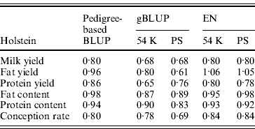
Table 6 presents the number of SNPs with a non-null effect retained by EN algorithm without or with a pre-selection of SNP in the Holstein breed. Similar results were obtained in Montbéliarde and Normande (data not shown). The results for the six traits are given, as well as the average of the number of SNPs over the 25 traits available for the three breeds. The number of SNPs retained was dependent on the genetic architecture of the trait. Traits such as Fat content where DGAT1 explains a very high part of the variance required fewer SNPs than conception rate. The mean number of SNPs over the 25 traits illustrates the impact of pre-selection on the number of retained SNPs.
Table 6. Correlation and number of SNP used in the prediction equation using the EN algorithm on the whole set of SNP (54 K) or after a pre-selection of the SNP (PS) for the Holstein breed

For the six presented traits, pre-selection led to a reduction of the number of SNPs needed in the prediction equation. Among these traits, conception rate is the one with the highest polygenic part as the number of SNPs included in the EN model shows. Production traits required between 1271 and 5648, which is much less than the 20 904 SNPs required for conception rate. The highest reduction of the number of SNPs retained was for conception rate (from 20 904 to 9677 SNPs, which corresponds to a reduction of 54%).
The impact of this SNP pre-selection on correlations was an absolute decrease limited to 1–2% and was relatively limited. For the 25 available traits, the average number of SNPs used in the prediction equation derived from the EN algorithm applied on the whole set of SNPs was 16 334. After pre-selection, this number declined to 10 059. This important decrease in the number of SNPs used was obtained while correlations remained relatively stable (loss of 1% on average). Surprisingly, for some traits, the number of SNPs retained by EN after pre-selection was higher than when EN was applied to the whole set of SNPs. This was the case for body depth, chest width and milking speed for Holstein. Nevertheless, this phenomenon was marginal and, for most traits, pre-selection allowed a large decrease in SNP numbers. The results presented in Table 6 correspond to the optimal α and λ values. During the EN procedure, a large number of parameter combinations were tested and some suboptimal combinations required an even smaller number of SNPs. Table 7 presents, for the Holstein breed and for the six initial traits, the highest correlations that were observed when the total number of SNPs with non-null effect was limited to a value between 2500 and 1000 SNPs. An option of the R package glmnet allows the maximum number of variables to be set. This option acts on the intensity of the penalization to validate this constraint.
Table 7. Highest correlation and corresponding number of selected SNPs when using the whole set of SNP (54 K), after a pre-selection of the SNP (PS) or when the number of selected SNPs is limited to 2500, 1500 or 1000 in the Holstein breed

Obviously, this limitation in the number of SNPs led to a decrease in correlation, but this was relatively limited: between 0 and 3·4% depending on the trait and the maximum number of SNPs defined. In complement to this table, Figure 1 presents the mean change in correlation over the 25 traits for the three breeds according to the number of selected SNPs.
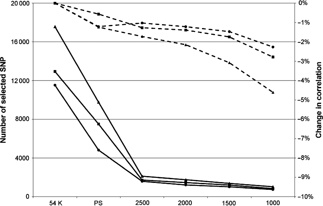
Fig. 1. Mean change in correlation (dashed lines) over the 25 traits for Montbéliarde (▪), Normande (•) and Holstein (▴) when the maximum number of SNPs selected by EN is restricted to the value indicated on the x-axis. Continuous lines represent the actual number of selected SNPs.
The breed found to be the most sensitive to the limitation of selected SNP in EN was the Holstein breed, but this is also the breed in which, on average, the largest number of SNPs without pre-selection are retained (17 341 selected SNPs in this situation against 11 526 in Normande and 12 939 in Montbéliarde). When the number of selected SNPs was limited to 2500, the average absolute loss in correlation over the 25 traits ranged from 1 and 1·7%. This average loss in correlation changed to 2·3 and 4·5% with a limit to 1000 selected SNPs.
4. Discussion
As for many previous studies, genomic evaluations with gBLUP and EN substantially improved the quality of prediction of observed DYD in the validation data set compared with pedigree-based BLUP (Hayes et al., Reference Hayes, Bowman, Chamberlain and Goddard2009; Wolc et al., Reference Wolc, Stricker, Arango, Settar, Fulton and O'Sullivan2011). Between these two genomic evaluations, gBLUP has the advantage of being conceptually simpler in the sense that there is no extra parameter to define or to optimize. In theory, a method that estimates all SNP effects should ensure that false-positive or uninformative effects are regressed towards zero, but in practice, these false positive or uninformative effects are not strictly equal to zero. EN, which shares some variable selection properties with other methods (like Bayes B, Cπ, …) limits the number of SNPs with non-null estimated effects in the model. This property can be an advantage because it alleviates the p>>n problems, in particular for smaller breeds. Limiting the number of SNP effects to estimates becomes important for an accurate prediction equation.
Since this study shows that EN provides better results than gBLUP for most traits in the three breeds studied, we tried to push further the idea of variable selection both in the case of gBLUP and EN by adding an SNP pre-selection step based on QTL detection. The resulting correlations between DGV and observed DYD and also the slopes of the regression of observed DYD on DGV were similar to the ones obtained using the complete set of SNPs. Moreover, both the EN algorithm and the pre-selection of the SNP led to a reduction of the number of SNPs included in the prediction equation with a minor effect on the quality of prediction. This procedure seems particularly relevant in the genomic selection context for two reasons:
• From a genetic standpoint, it is consistent with the assumption that not all SNPs are required to explain the genetic architecture of a given trait. Some of them, with non-significant effects, can still carry genetic information and particularly on genetic relationships (Habier et al., Reference Habier, Fernando and Dekkers2007, Reference Habier, Tetens, Seefried, Lichtner and Thaller2010b). However, since very similar correlations were obtained using the complete set of SNPs or a fraction of them after pre-selection, it means that a subset of SNPs included in the model was not really informative for the trait and pre-selection avoids including in the prediction equation these uninformative SNPs.
• Furthermore, it is expected that in the near future the number of genotyped animals and the number of SNPs will get larger and larger. This will represent a major challenge for genomic evaluations from a computing point of view. The SNP pre-selection implemented here requires an LDLA approach and a detection of the LRT peak, which is based on two parameters (windows of SNP to consider and an LRT threshold). The LDLA approach requires phasing the data which, depending on the methodology used, could be computationally time consuming. However, the LDLA approach does not have to be performed at each genomic evaluation because animals that are added between two genomic evaluations are young and their performances have a very low weight compared with older ones. Moreover, as mentioned before, the time-consuming step is to phase the data. Actually, this step is not required for all the genomic selection methods used in national evaluation and consequently, constraints due to phasing data are not encountered. But if an additional imputation step is required to mix different versions of chips (Illumina Bovine SNP50 BeadChip® V1 and V2 for example) or different sizes of chips (3, 50 and 777 K), this phasing step is routinely needed anyway. Then, SNP pre-selection strongly alleviates computing requirements and consequently ensures that national evaluations can be completed within a reasonable time frame.
In this study, we focused on one variable selection method that is the EN and one pre-selection method that is LDLA. Obviously, other genomic selection methods (Bayesian methods for instance) and other pre-selection approaches (based on ‘pure’ association studies instead of LDLA for instance) should be also tested to complete this study. EN provided better results in our study and our model assumed that all genetic variation was explained by SNP. The latter may be true if all causal mutations are bi-allelic and if SNPs are in strong linkage disequilibrium with all causal mutations. If causal mutations are multi-allelic or if SNPs are in weak linkage disequilibrium with this causal mutation, model based on haplotypes could be more advantageous. The current French genomic evaluation (Boichard et al., Reference Boichard, Guillaume, Baur, Croiseau, Rossignol and Boscher2010) combines Marker Assisted Selection (MAS) on QTL followed through haplotypes and genomic selection based on SNP detected with the EN algorithm. EN was used as a variable selection method and prediction equations were generated for the French genomic MAS.
In conclusion, the EN algorithm appears to be a very flexible and promising tool in the genomic selection framework that can be used for genomic evaluation or as a variable selection device to provide SNP of interest to a marker-assisted evaluation method.
This work was part of the AMASGEN project within the ‘UMT évaluation génétique’ financed by the French National Research Agency (ANR) and by ApisGene. Labogena is gratefully acknowledged for providing the genotypes.
Declaration of Interest
None.


