1. Introduction
Traditionally selection to improve profitability of livestock production has been based on phenotypic and pedigree information. However, the availability of dense single nucleotide polymorphisms (SNPs) and dramatic reduction in the cost of acquiring this information has allowed the inclusion of genome wide marker information in the prediction of animals' breeding values.
Meuwissen et al. (Reference Meuwissen, Hayes and Goddard2001) introduced genomic selection as a selection strategy based on genomic breeding values predicted from dense marker data. The method implicitly recognized the fact that quantitative traits such as those affecting profit of livestock production are controlled by the segregation of large numbers of multiple quantitative trait loci (QTLs), and therefore predicts an animal's breeding value by simultaneously evaluating and summing large numbers of marker effects across the entire genome. The method makes the assumption that the markers are in linkage disequilibrium (LD) with the QTL. The higher the density of the markers is, the greater the level of LD between the markers and the QTL and thus the greater proportion of genetic variance that can be explained by the markers.
In the reference population, where the SNP effects are predicted, the number of marker effects (p) to simultaneously estimate will typically be substantially larger than the number of animals genotyped (n), which leads to the difficulty of an over-saturated model (i.e. p>n). Thus, a model for genomic selection must be able to overcome this problem. The other necessity is a sparse model because of the large number of SNP effects that are zero or close to zero. Subsequently, a crucial question is how to decide whether an SNP is in, or out of the set of SNPs chosen to give the most accurate prediction of breeding values in independent data sets. One potential approach is to use shrinkage methods such as the least absolute shrinkage and selection operator (LASSO), where all SNPs are included in the predictive set but the smaller effects are shrunk back towards zero (Tibshirani, Reference Tibshirani1996). Another approach is to use the reversible jump Markov chain Monte Carlo (MCMC) algorithm (Green, Reference Green1995), which uses a variable dimension model space approach that allows the SNPs in the predictive set to change. Stochastic search variable selection (SSVS) (George & McCulloch, Reference George and McCulloch1993) provides a method to maintain a constant dimensionality across all models but allows the SNPs in the predictive set to change. It allows this by instead of removing all non-significant parameters (those that would be excluded from the predictive set using the reversible jump algorithm) from the model, their effects are limited to values very close to zero.
The major advantage of this method is that the posterior distribution of all parameters can be sampled directly using the Gibbs sampler, instead of using more computationally demanding algorithms such as the reversible jump algorithm. SSVS has been previously used for identifying multiple QTLs (Yi et al., Reference Yi, George and Allison2003), multivariate regression models (Brown et al., Reference Brown, Vannucci and Fearn1998), gene mapping (Swartz et al., Reference Swartz, Kimmel, Mueller and Amos2006) and generalized linear models (George & McCulloch, Reference George and McCulloch1997). It has also been utilized for analysing multi-trait QTL mapping data (Meuwissen & Goddard, Reference Meuwissen and Goddard2004), and subsequently to investigate the effect that different methods for defining haplotypes and the effect of the inclusion of the polygenic effect had on the accuracy of genomic selection in simulated data (Calus et al., Reference Calus, Meuwissen, de Roos and Veerkamp2008; Calus & Veerkamp, Reference Calus and Veerkamp2007).
In this paper, we demonstrate that a Bayesian SSVS can be used effectively when compared with other methods for genomic selection using real SNP data. It also provides an viable alternative to more computationally demanding approaches such as Bayes B (Meuwissen et al., Reference Meuwissen, Hayes and Goddard2001).
2. Materials and methods
(i) SNP data
The data set contained 1498 Australian Holstein-Friesian bulls genotyped for the Illumina Bovine50K array. After quality control, 39 048 SNPs remained in the predictive set. The quality control applied to the SNP data is described by Hayes et al. (Reference Hayes, Bowman, Chamberlain and Goddard2009). The reference data set where the SNP effects were predicted contained 1098 bulls born between 1940 and 2000. The phenotypes for these bulls were Australian breeding values (ABV) for protein kg, fat kg, protein percentage, fat percentage and daughter fertility, all deregressed to remove any contribution from relatives (Hayes et al., Reference Hayes, Bowman, Chamberlain and Goddard2009). Daughter fertility here is defined as the difference between bulls for the percentage of their daughters pregnant 6 weeks after mating start date or 100 days after calving in year-round herds. The validation set contained 400 genotyped bulls proven from the years 2005, 2006 and 2007 with ABV which included information from at least 100 milking daughters to enable comparison with predicted marker estimated breeding value (MEBVs).
(ii) Model
At each locus (total number of loci, p) there are three possible combinations of two alleles (e.g. A or B), the homozygote of one allele (AA), the heterozygote (AB) and the homozygote of the other allele (BB). These are then quantitatively represented by 0, 1 and 2, respectively. The model fitted to the above data was then
where y is the vector of phenotypes of the trait being analysed for all n individuals, μ is the mean, 1n is a vector of ones of length n, Xj is a vector of indicator variables representing the genotypes of the jth marker for all individuals (xij =0, 1, 2), βj is the size of the QTL effect associated with marker j, u is the vector of random polygenic effects of length n (Z is the associated design matrix) and is assumed to be normally distributed, u~N(0, σu2A) and e is the residual error also assumed to be normally distributed, e~N(0, Iσe2). The polygenic effect was included to remove the effect of population structure to enable more accurate estimation of the SNP effects. Its inclusion has been shown to produce slightly better accuracies of prediction while reducing the bias of the variance components (Calus & Veerkamp, Reference Calus and Veerkamp2007).
(iii) SSVS
The key feature of SSVS compared with Bayes A or B (Meuwissen et al., Reference Meuwissen, Hayes and Goddard2001) is the introduction of a latent or indicator variable, γ, into the hierarchical model. This enables the extraction of information relevant to variable selection. The latent variable can take either 1 or 0, representing whether the SNP is included as a significant effect in the model or not. As such, the prior distribution for each SNP effect is a normal mixture conditional on the corresponding γ and the variance that is sampled from an inverse scaled chi-square distribution:
At the SNP effect level, this hierarchical prior distribution specification means the SNP effects are sampled from a mixture of two-student t distributions. The values of r and S were calculated as in Meuwissen et al. (Reference Meuwissen, Hayes and Goddard2001). The prior distribution of the indicator variable is chosen to reflect the belief of whether an SNP is linked to a QTL. The probability of an SNP being sampled from the smaller or larger distribution is
Subsequently, the prior distribution for the indicator variable is a Bernoulli distribution:
The prior probability pi is chosen to reflect the information available on how many QTLs affect the trait of interest. It can be quantified as the number of SNPs expected to be linked to a QTL divided by the total number of SNPs. In genome-wide association studies or genomic selection applications, the expected proportion of QTLs can be reasonably estimated based on knowledge about the trait of interest and previous QTL studies results.
The posterior distribution of the indicator variable can be sampled directly using

where γ−i is all terms of γ except γi.
The frequency that each SNP appears in the model is shown by the posterior distribution of the indicator variable. SNPs that are included in the model frequently have a high posterior probability and will most likely be linked to a QTL.
(iv) Additional methods
Bayes A, Bayes B and BLUP were also run on the data. Bayes A and Bayes B were as specified in Meuwissen et al. (Reference Meuwissen, Hayes and Goddard2001) with the addition of a polygenic effect. A Bayesian BLUP method was also implemented. It is identical to the specification of Bayes A with the exception that all SNPs had a constant equal variance that was sampled once each iteration from an inverse-scaled chi-square distribution.
In order to have Bayes B results for comparison with Bayes SSVS, we also used a modified version of Bayes B approach. The modified version consisted of running Bayes B cycles with the Metropolis Hastings (MH) algorithm every 100 iterations of Bayes A. (Note the Jacobian in the acceptance ratio of the reversible jump algorithm was equal to one thus identical to the MH algorithm). If an SNP effect was found to be zero during these MH iterations then it was set to zero during the subsequent Bayes A cycles. This effectively maintained the same assumptions as Bayes B, while significantly reducing the time required to reach convergence.
(v) Breeding values
MEBVs for bulls in the validation data set were calculated as the sum of the mean, the effects of the SNP genotypes it carried and the polygenic effect, ![]() . The accuracy of the methods were evaluated on the correlation, the mean square error (MSE) and the regression coefficient of the ABV (assumed to be the true breeding value) on the predicted MEBV. Genomic selection aims to produce breeding values as close as possible to the true breeding value. The ABV was used for comparison as it is a most accurate predictor of the true breeding value and it is regressed according to the amount of information available.
. The accuracy of the methods were evaluated on the correlation, the mean square error (MSE) and the regression coefficient of the ABV (assumed to be the true breeding value) on the predicted MEBV. Genomic selection aims to produce breeding values as close as possible to the true breeding value. The ABV was used for comparison as it is a most accurate predictor of the true breeding value and it is regressed according to the amount of information available.
3. Results and discussion
(i) Time to convergence
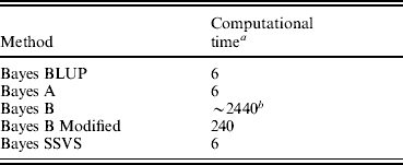
All methods were run for 10 000 iterations to ensure convergence. This number of iterations was shown to be sufficient for convergence with formal diagnostic methods provided in the package R, coda (Plummer et al., Reference Plummer, Best, Cowles and Vines2007). The use of the SSVS method is analogous to Bayes B in the assumption that the majority of the SNP effects are thought to be very small and insignificant. However, as illustrated in Table 1, the fixed dimensions of the model used in SSVS allow the use of the Gibbs Sampler that is significantly computationally less demanding and consequently quicker than the reversible jump MCMC algorithm or the MH algorithm used in traditional Bayes B. Given the very high computational demand of Bayes B, it was not possible to run this algorithm to convergence. The time to convergence was extrapolated from running Bayes B for 1000 iterations. The Bayes A and Bayes BLUP methods reached convergence in comparable times to Bayes SSVS.
Table 1. Computational time for genomic selection methods

a Processor clock hours.
b Estimated time to convergence.
(ii) Comparison of Bayes B and Bayes SSVS results
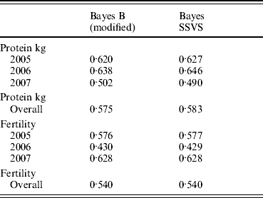
The correlations between the ABVs and the MEBV predicted for the animals in the validation set by the modified Bayes B and Bayes SSVS for fertility and protein kg traits are shown in Table 2. This shows that the two methods produce almost identical correlations with the ABVs as expected. The MEBV for the two methods are 99·9 and 98·0% correlated for protein and fertility, respectively. This equivalence in results demonstrates that the Bayes SSVS method does maintain the SNP effect assumptions of the original Bayes B and produce near to identical results. The slightly lower result for fertility is probably due to the non-normality of the trait making it harder to estimate and by the modification of the original Bayes B. The modified Bayes B produced not significantly different but slightly larger MSEs and regression coefficients (results not shown). This is most likely due to the modification to reduce the computational time to convergence. The time taken for the modified version of Bayes B was still 40-fold larger than for the Bayes SSVS that produced identical accuracies (see Table 1).
Table 2. Correlation between predicted MEBV and ABV for proven bulls (years 2005, 2006, 2007 and overall) for the modified Bayes B and Bayes SSVS

(iii) Comparison of BLUP, Bayes A, Bayes SSVS results
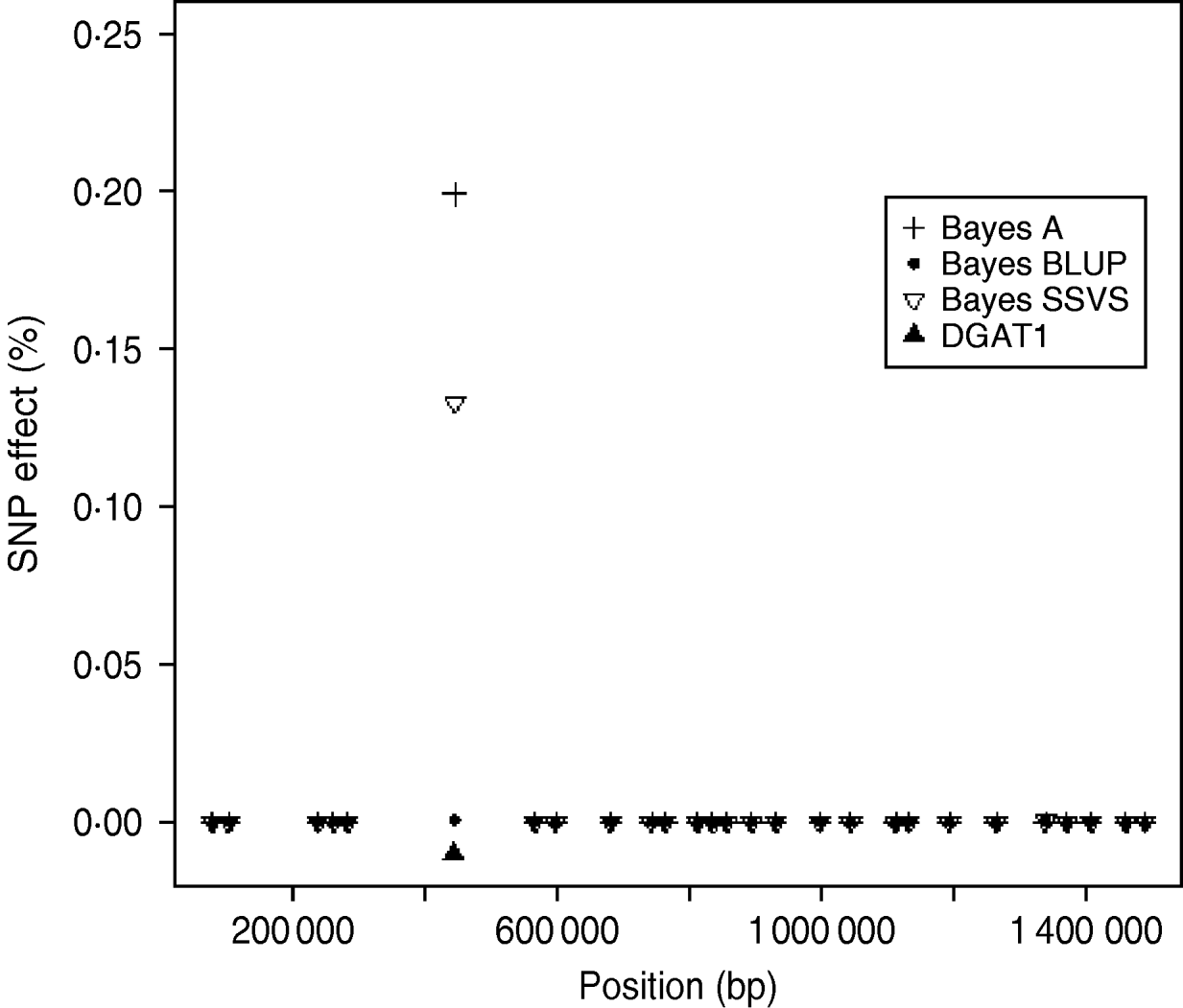
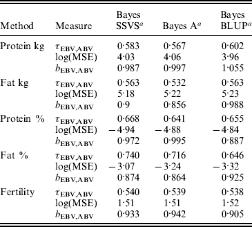
The logarithm of the MSE, regression and correlation coefficients for the predicted MEBV and ABV for the traits fertility protein kg, fat kg, protein percentage and fat percentage are shown in Table 3. The values shown are the average values for the proven bulls in the years 2005, 2006 and 2007 from the validation data set. BLUP has the highest overall correlation and the lowest MSE between the three methods for protein kg. For the traits, fat kg and protein percentage, Bayes SSVS produces the highest correlations and has the lowest bias; however, there are no significant differences between methods. However, there are significant differences between the methods for fat percentage. These difference in the method accuracies across traits or the apparent ‘trait by method’ interactions can be explained by the distribution of QTLs for the different traits. For example, protein kg has no known genes of large effect and thus BLUP, which uses equal variances across all SNPs, can be used successfully to accurately predict breeding values. In contrast, fat percentage has a known mutation, DGAT1, that is common and acts additively and is known to be responsible for explaining a large percentage of genetic variation for the trait (Grisart et al., Reference Grisart, Coppieters, Farnir, Karim and Ford2002). The individual SNP variances that Bayes A and Bayes SSVS uses, allows effects of a large size not to be penalized (shrunk) as severely as in BLUP. This is clearly shown in Fig. 1, where the percentage each SNP contributes to the total SNP effects are plotted for the three methods for the centromeric end of the bovine chromosome 14. Bayes A and Bayes C have an SNP with an effect significantly greater than zero, while the Bayes BLUP effects for SNP near DGAT1 and surrounding the mutation are close to zero. Bayes SSVS does perform slightly better than Bayes A for fat percentage. The advantage of the Bayes SSVS over Bayes A may be the prior structure consisting of two distributions: a distribution of larger significant effects and a smaller distribution close to zero. This allows the SNP with larger effects to have values in their posterior sampled from the larger distribution, while those SNPs without significance have their effects sampled from the smaller posterior distribution of values very close to zero. Traits with large effects will be more accurately predicted using SSVS than Bayes A as the prior structure allows more variance to be attributed to the larger effects.

Fig. 1. SNP effects (%) for fat percentage from Bayes A, Bayes BLUP and Bayes C found on the centromeric end of chromosome 14.
Table 3. MSE, correlation and regression coefficient between predicted MEBV and ABV in the validation data set

a Average accuracies reported over validation sets from years 2005, 2006 and 2007.
τEBV,ABV, correlation coefficient between the ABV and the predicted MEBV.
log(MSE) is the logarithm of the MSE between the ABV and the predicted MEBV.
b EBV,ABV, regression coefficient of the ABV on predicted MEBV.
4. Conclusion
Bayesian SSVS produced more accurate MEBV for most of the dairy traits in our data set than other methods. The comparison with a modified version of Bayes B showed that it is equivalent and produces the same results with dramatically less computational time required. For traits with a mutation of known large effect such as fat percentage, Bayes SSVS gave significantly higher accuracy of MEBV than the BLUP method as expected given that its prior is closer to the real distribution of effects than that of BLUP. The use of an indicator variable in Bayes SSVS would also allow the premeditated inclusion of SNPs in a model that are known to be linked to QTL of biological importance. Instead of using a single value to set the prior probability for all SNPs a vector of probabilities could be used as prior probabilities to allow more prior information to be included should it be available. Overall, this study has shown that the Bayes SSVS method provides reduced computational time and accurate results when using real dairy data to predict genomic breeding values and provides a viable alternative to other Bayesian methods for genomic selection.
The authors would like to thank Mehar Khatkar and Herman Raadsma for provision of part of the data used in this paper.


