


Impact Statement
It has recently been proposed that environmental structures such as trees can be used as ubiquitous, low-cost flow sensors by leveraging visual observations of their characteristic responses to wind loading (Reference Cardona, Bouman and DabiriCardona, Bouman, & Dabiri, 2021). Potential application areas include analyses of pollution dispersal and wildfire propagation. The present work demonstrates that measurements of tree sway amplitudes can be related to wind speeds in the context of this visual anemometry goal. This greatly expands the potential of visual anemometry methods to be used on a broad variety of trees and in lower-speed wind conditions, since it does not require that trees exhibit large observable mean bending.
1. Introduction
Recent work has suggested that flow speeds can be measured using visual observations of flow–structure interactions such as the bending response of trees to incident wind (Reference Cardona, Bouman and DabiriCardona et al., 2021; Reference Cardona, Howland and DabiriCardona, Howland, & Dabiri, 2019). Video of trees could potentially be used instead of conventional point-wise anemometers to achieve low-cost, spatially resolved wind speed measurements simultaneously throughout the entire camera field of view. Such data would be valuable for applications such as analyses of pollution dispersal and wildfire propagation. Reference Cardona, Bouman and DabiriCardona et al. (Reference Cardona, Bouman and Dabiri2021) presented a technique that allowed for normalized wind speed measurements to be made using mean structural deflections compared with a known reference condition. The aforementioned method demonstrated how visual observations of objects including trees can be used toward anemometry tasks. However, the application of that method requires that the mean deflections can be observed, which may not always be possible or convenient in practice. Mean deflections may be small in many cases, especially for large trees, making them difficult to measure accurately. For instance, a field study by Reference Peltola, Kellomäki, Hassinen and LemettinenPeltola, Kellomäki, Hassinen, and Lemettinen (Reference Peltola, Kellomäki, Hassinen and Lemettinen1993) found that for two Scots pines of 9.5 and 13.5 m tall, the maximum bending measurements at the crown centre heights were less than 2 and 5 cm, respectively, for a wind speed range of 4–8 m s $^{-1}$. The amount of static bending that a tree undergoes is a function of its slenderness and material properties in addition to the wind (discussed further in § 2.3). This limits the range of trees and wind conditions for which the mean bending method proposed by Reference Cardona, Bouman and DabiriCardona et al. (Reference Cardona, Bouman and Dabiri2021) can be used. Another challenge is that mean deflections must be measured with respect to the object position under no wind load. This inherently means that the object must be observed in the absence of wind in addition to being observed under a known calibration wind speed.
Trees are desirable target objects to use for visual anemometry because of their ubiquity. For instance, in New York City, more than  $680\,000$ trees have been mapped to date, with 234 species represented (NYC Parks, 2021). A tree-based visual anemometry method will be most widely applicable to wind mapping applications if it can be used on a diverse range of trees of various sizes and species. Although the mean deflection-based technique developed by Reference Cardona, Bouman and DabiriCardona et al. (Reference Cardona, Bouman and Dabiri2021) is limited in this regard, the behaviour of a tree in response to incident wind is dynamic, and is rich with information extending beyond the mean deflections. For example, the land adaptation of the Beaufort scale relies on perceptible tree branch motion as a correlate for low wind speeds (Reference JemisonJemison, 1934). Tree motion has previously been related to the time-varying wind speed, often through semi-empirical mechanical transfer functions (Reference Holbo, Corbett and HortonHolbo, Corbett, & Horton, 1980; Reference Kerzenmacher and GardinerKerzenmacher & Gardiner, 1998; Reference MayerMayer, 1987; Reference Moore and MaguireMoore & Maguire, 2008). These transfer functions depend on the tree-specific properties affecting the dynamics, including the natural frequency, damping and drag coefficient. Prior work measuring tree sway also suggests that the magnitude of the tree sway increases with increasing wind speed (Reference Peltola, Kellomäki, Hassinen and LemettinenPeltola et al., 1993; Reference van Emmerik, Steele-Dunne, Hut, Gentine, Guerin, Oliveira and Van De Giesenvan Emmerik et al., 2017), as does the velocity of the tree branches (Reference Tadrist, Saudreau, Hémon, Amandolese, Marquier, Leclercq and de LangreTadrist et al., 2018).
The present work leverages dynamic tree sway to extend the capabilities of the visual anemometry technique proposed by (Reference Cardona, Bouman and DabiriCardona et al. 2021). A physical model is developed, applying a force balance to relate mean wind speeds to the amplitude of tree sway. This eliminates the need to observe the object of interest in the absence of wind loading, and allows measurements to be made in cases where swaying behaviour is observable even when mean deflections are difficult to measure. The model is applied to two field datasets including a video dataset capturing the swaying behaviour of a M. grandiflora in an open field, and a publicly available dataset with strain gauge measurements of 12 trees of 3 different species in a broadleaf forest in the UK (Reference JacksonJackson, 2018). Results suggest that the method developed in this work is widely applicable to a diverse set of trees.
2. Methods
2.1 Analytical model
The structural deflection,  $\delta$, in response to wind loading was modelled based on Newton's law for a single degree of freedom damped harmonic oscillator
 \begin{equation} F_W(t) = m \ddot{\delta} + \lambda \dot{\delta} + \kappa \delta, \end{equation}
where  $F_W$ is the external forcing due to incident wind, $m$ is the mass of the structure, $\lambda$ is the damping coefficient and $\kappa$ is the elastic constant. An arbitrary time-dependent forcing $F(t)$ can be expressed as a Fourier series
 \begin{equation} F(t) = \frac{a_0}{2} + \sum^{\infty}_{n = 1} (a_n \cos(nt)) + \sum^{\infty}_{n = 1} (b_n \sin(nt)). \end{equation}
When forced with harmonic loading,
 \begin{equation} F(t) = F_0 \sin(\omega t), \end{equation}
where  $\omega$ is the forcing frequency, and $t$ is time, the steady-state solution of (2.1) is
 \begin{equation} \delta(t) = \frac{F_0}{\kappa} \left[ \frac{1}{(1-\beta^2) + (2 \zeta \beta)^2} \right] \left[ (1-\beta^2) \sin(\omega t) - 2\zeta \beta \cos(\omega t) \right], \end{equation}
where  $\beta$ is the ratio of the forcing frequency to the natural frequency of the system $(\beta = \omega /\omega _n)$, and $\zeta = {\lambda }/{2\sqrt {\kappa m}}$ (Reference Clough and PenzienClough & Penzien, 1995).
In the present work, we define the amplitude of the structural oscillations as the standard deviation of the structural deflection,  $\sigma (\delta )$ (median absolute deviation is discussed as an alternative to this choice in the supplementary material, § S1.2 is available at https://doi.org/10.1017/flo.2021.15). The steady-state solution given by (2.4) reveals that the amplitude of structural oscillations scales with the forcing amplitude
 \begin{equation} \sigma(\delta(t)) \propto \sigma(F_W(t)). \end{equation}
 The instantaneous force of the wind on the structure,  $F_W$, is given by
 \begin{align} F_W(t) &\propto \rho A U^2(t) \end{align}
 \begin{align} & = CU^2(t), \end{align}
where  $\rho$ is the fluid density, $A$ is the projected frontal area of the structure, $U(t)$ is the instantaneous wind speed and $C$ is a positive constant. The instantaneous wind speed, $U(t)$, can be decomposed as a sum of the mean wind speed, $\bar {U}$, and the unsteady fluctuating wind speed, $u'(t)$. This gives
 \begin{align} F_W(t) & = C [\bar{U} + u'(t)]^2 \nonumber\\ & = C [\bar{U}^2 + 2\bar{U}u' + u'^2]. \end{align}
Taking the standard deviation of (2.8) gives an expression relating  $\sigma (F_W)$ to $\bar {U}$ and $u'$
$u'$
 \begin{align} \sigma(F_W) & = \sigma ( C [\bar{U}^2 + 2\bar{U}u' + u^{\prime 2}] ) \nonumber\\ & = C \sigma ( \bar{U}^2 + 2\bar{U}u' + u^{\prime 2}) \nonumber\\ & = C \sigma (2\bar{U}u' + u^{\prime 2}),\end{align}
or equivalently
 \begin{equation} \sigma(F_W) \propto \sigma(2\bar{U}u' + u'^2). \end{equation}
 Assuming  $u'/\bar {U} \ll 1$, the $u'^2$ term in (2.10) can be neglected, giving
 \begin{align} \sigma(F_W) &\propto \sigma( 2\bar{U}u') \nonumber\\ &\propto \sigma(\bar{U}u') \nonumber\\ &\propto \sigma(u')\bar{U} \nonumber\\ &\propto \frac{\sigma(u')}{\bar{U}} \bar{U}^2. \end{align}
The assumption that  $u'/\bar {U} \ll 1$ is examined in field measurements described below. The turbulence intensity, ${\sigma (u')}/{\bar {U}}$, will be denoted as $I_u$. Given that the structural sway amplitude, $\sigma (\delta )$, scales with $\sigma (F_W)$ (2.5), $\sigma (\delta )$ can replace $\sigma (F_W)$ in (2.11), yielding
 \begin{equation} \sigma(\delta) \propto I_u \bar{U}^2. \end{equation}
The simplified final expression given in (2.12) reveals that the sway amplitude scales with  $\bar {U}^2$ multiplied by the turbulence intensity $I_u$.
2.2 Field measurements
Analysis was carried out on two distinct datasets: a direct field measurement dataset comprising videos of a M. grandiflora collected for the purposes of this work, and an indirect field measurement dataset comprising strain gauge data for several trees collected by Reference JacksonJackson (Reference Jackson2018). Methods are described for each of these two datasets in §§ 2.2.1 and 2.2.2, respectively. The direct field measurements from the videos of the M. grandiflora are used to demonstrate model application to visual observations of dynamic oscillations. Model generalizability to a diverse set of trees is established through its application to the indirect field measurements from Reference JacksonJackson (Reference Jackson2018).
In total, 13 trees across 4 different species were analysed between the two datasets. The four species considered were: M. grandiflora (magnolia), Fraxinus excelsior (ash), Betula spp. (birch) and Acer pseudoplatanus (sycamore). The tree species are henceforth referred to by their common names. Table 1 lists the approximate height,  $h$, diameter at breast height, DBH, and elastic modulus, $E$, for each of the 13 test trees. Tree ID numbers are also listed for the subset of trees from the Reference JacksonJackson (Reference Jackson2018) dataset for reference. Approximate values of $E$ were obtained from literature-reported values (Reference Green, Winandy and KretschmannGreen et al., 1999; Reference Niklas and SpatzNiklas & Spatz, 2010).
Table 1. Summary of the properties of the 13 test trees analysed in the present work, including species, height ( $h$), diameter at breast height (DBH) and approximate elastic modulus ( $E$). Literature-reported values of $E$ were obtained from $^{a}$Reference Green, Winandy and KretschmannGreen, Winandy, and Kretschmann (Reference Green, Winandy and Kretschmann1999) and $^{b}$Reference Niklas and SpatzNiklas and Spatz (Reference Niklas and Spatz2010). Tree ID numbers assigned in the original Reference JacksonJackson (Reference Jackson2018) dataset are also listed for the relevant subset of trees.

2.2.1 Direct field measurements
Observations of the dynamic sway of a magnolia tree were captured in 1 min video clips recorded in an open field with flat terrain in Lancaster, California in the USA. This test tree was the same specimen that was used by Reference Cardona, Howland and DabiriCardona et al. (Reference Cardona, Howland and Dabiri2019) to train a machine learning model. A photo of the tree is shown in figure 1(a), and tree properties are listed in table 1. The data were collected during August, 2018, during daylight hours when the lighting conditions allowed for the treetop to be easily tracked. Videos were recorded at 15 frames per second (f.p.s.). A  $150 \times 150$ pixel (px) region of interest capturing the top of the tree was used for analysis. To measure the deflection, the frames were binarized to distinguish the tree from the background, and the top-most pixel of the tree was tracked over time. The deflection, $\delta (t)$, was measured by calculating the displacement in the horizontal direction in each frame relative to the mean position over the 1 min period (900 frames). Note that sensitivity to the averaging period is discussed further in the supplementary material (§ S1.3). An example of a binarized frame with the treetop detected is shown in figure 1(b). Deflection, $\delta$, was measured at integer pixel resolution. Figure 1(c) illustrates how $\delta$ would be measured between an original and deflected position of the tree. A timetrace of $\delta (t)$ is shown in figure 1(d), along with the distribution of $\delta$ over a 1 min averaging window (figure 1e).

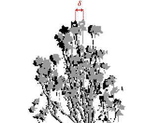
Figure 1. (a) The M. grandiflora specimen used for analysis. (b) An example of a cropped and binarized image of the treetop. The top-most point on the tree (marked here with the green ‘+’) was located in each frame for tracking in order to measure  $\delta (t)$. (c) An example of how $\delta$ would be measured between an original position (black) and deflected position (grey) of the treetop. Note that, although the deflection is shown between two video frames here for illustration, $\delta$ was calculated with respect to the mean position of the treetop over the 900 frames for each video. (d) Plot of $\delta$ vs. time for a representative 1 min video clip ( $\bar {U} = 9.17$ m s $^{-1}$). The grey band shows $\pm \sigma (\delta )$. As noted in § 2.1, $\sigma (\delta )$ was used to quantify the sway amplitude for these video experiments. (e) Probability density function (PDF) of measurements of $\delta$ taken during the averaging window.
Wind speeds were recorded with an anemometer on site (Thies First Class) positioned at 10 m height and located approximately 60 m from the tree. In selecting time periods to analyse, the incident wind direction was fixed at  $250^\circ \pm 10^\circ$, which is approximately 50 $^\circ$ from the plane of the recorded images. This allowed for video clips to be compared without correcting for changes in incident wind direction with respect to the camera angle. The turbulence intensity varied from 10 % to 12 % during experiments, consistent with an assumed approximately constant value of $I_u$ in (2.12).
2.2.2 Indirect field measurements
The dataset collected by Reference JacksonJackson (Reference Jackson2018) comprised strain gauge data for 21 broadleaf trees located in Wytham Woods, a broadleaf forest in southern England. Each tree was instrumented with a pair of perpendicular strain gauges installed at 1.3 m height on the trunk. Strain gauge data were recorded at 4 Hz. The dataset also included wind data collected in a walkway within the forest canopy with a cup anemometer at a time resolution of 0.1 Hz. The present analysis focuses on a subset of data collected during winter months (January–February, 2016) corresponding to the absence of foliage for these species of broadleaf trees as noted by Reference Jackson, Shenkin, Wellpott, Calders, Origo, Disney and MalhiJackson et al. (Reference Jackson, Shenkin, Wellpott, Calders, Origo, Disney and Malhi2019). The subset of 12 trees considered in this work are listed in table 1 along with their approximate dimensions.
The model given in (2.12) is based on deflection,  $\delta$, but it can be equivalently applied to the bending strain, $\varepsilon$, measured from the strain gauges. Bending strain in an idealized cantilever beam is given by
 \begin{equation} \varepsilon = \frac{Mc}{EI}, \end{equation}
where  $M$ is the bending moment, $c$ is the distance from the neutral axis, $E$ is the elastic modulus and $I$ is the area moment of inertia. For a cantilever beam subject to a uniform distributed load, the bending moment, $M$ is given by
 \begin{equation} M = \frac{fx^2}{2}, \end{equation}
where  $f$ is the force per unit length and $x$ is the position along the length of the beam. The tip deflection is given by
 \begin{equation} \delta = \frac{fL^4}{8EI}, \end{equation}
where  $L$ is the length of the beam. The strain, $\varepsilon$, and tip deflection, $\delta$, both scale with the force per unit length, $f$. Thus, the strain is proportional to the tip deflection ( $\varepsilon \propto \delta$) for a given loading, and the strain gauge measurements can be used directly in the model in place of the tip deflections. The standard deviation of $\varepsilon$ is used to define the sway amplitude for analyses of the strain gauge dataset, and in this case the model relating sway amplitude and wind speed is
 \begin{equation} \sigma(\varepsilon) \propto I_u \bar{U}^2. \end{equation}
 To compare experimental results with the physical model, sway amplitudes, mean wind speeds, and turbulence intensities were quantified from the Reference JacksonJackson (Reference Jackson2018) dataset over 10 min averaging periods. Note that this averaging period is longer than the 1 min period used for the video dataset (§ 2.2.1). This longer averaging period was afforded by the abundance of available data. We observed improved model agreement using the longer, 10 min averaging windows (this is discussed further in the supplementary material, § S1.3). Timestamps were matched to retrieve samples for which both anemometer-recorded wind data and strain gauge data were available over the course of the full 10 min averaging periods. The averaging periods did not overlap (i.e. each sample represented a unique window in time). Values of  $\bar {U}$ and $I_u$ were calculated from the instantaneous measurements of $U(t)$ for each averaging period. The strain, $\varepsilon (t)$, was calculated as
 \begin{equation} \varepsilon(t) = \sqrt{\varepsilon_N^2(t) + \varepsilon_E^2(t)}, \end{equation}
where  $\varepsilon _N$ and $\varepsilon _E$ are the strain measurements recorded by the northward and eastward oriented strain gauges comprising a perpendicular pair for a given tree. The instantaneous strain measurements, $\varepsilon (t)$, were used to calculate the sway amplitude, $\sigma (\varepsilon )$, for each averaging window. A representative example timetrace of the strain over a 10 min averaging window is shown in figure 2(a). The PDF of strain measurements over the averaging window is also shown (figure 2b).

Figure 2. Representative example of strain measurements over a 10 min averaging window for a sycamore tree (tree no. 17) with  $\bar {U}=1.08$ m s $^{-1}$. (a) Strain vs. time with the mean value shown with the black line and $\pm \sigma (\varepsilon )$ shown with the grey band. (b) The PDF of strain measurements taken during the averaging window.
2.3 Tree response regimes
The response of a tree subject to incident wind loading depends on both fluid and structural properties. The Cauchy number,  $Ca$, and slenderness ratio, $S$, are useful in determining whether a tree is likely to show large static bending (Reference de Langrede Langre, 2008). The parameters $Ca$ and $S$ are defined as
 \begin{align} Ca & = \frac{\rho U^2}{E}, \end{align}
 \begin{align} S & = \frac{L}{l}, \end{align}
where  $L$ and $l$ are the maximum and minimum dimensional lengths of the cross-section perpendicular to the flow direction respectively. Large static deformation is expected when $Ca S^3 > 1$ (Reference de Langrede Langre, 2008). Therefore, less slender trees will resist large observable static bending until higher wind speeds are reached. Values of $CaS^3$ were approximated for the trees analysed in this work. The lengths, $L$ and $l$, were taken to be the tree height ( $h$) and the DBH, respectively. The trees of interest in this study correspond to values of $CaS^3 \leq 5 \times 10^{-3}$, suggesting that large static deformations are not present. This limits the applicability of the mean bending method of Reference Cardona, Bouman and DabiriCardona et al. (Reference Cardona, Bouman and Dabiri2021).
3. Results
3.1 Model comparison with direct field measurements from video data
Figure 3 shows the mean wind speed plotted against the square root of the sway amplitude for the field measurements of the magnolia tree from the video dataset. Datapoints are shown for each of the 1 min video clips captured in the field experiments. The best-fit line assuming proportionality (i.e.  $\sqrt {\sigma (\delta )} \propto \bar {U}$) is shown with the black line (calculated using ordinary least squares). The experimental data agree well with the proportional model, with the best-fit line yielding $R^2 = 0.81$. These results demonstrate that the proposed physical model (i.e. (2.12)) characterizes the relationship between tree sway and mean wind speed captured in this video dataset.

Figure 3. Mean wind speed,  $\bar {U}$, vs. the square root of sway amplitude measured from video frames. Black lines indicate best fit for proportional model with $R^2$ value of 0.81.
3.2 Model comparison with indirect field measurements from strain gauge data
Figure 4 shows the mean wind speed versus the square root of the sway amplitude for each of the 12 trees analysed from the Reference JacksonJackson (Reference Jackson2018) dataset. In the engineering application employing the physical model for anemometry, both  $\bar {U}$ and $I_u$ would be unknown, and the oscillatory motion of the structure would be the sole experimentally measured quantity. Therefore, $I_u$ was not considered to generate these results (i.e. $I_u$ assumed constant). Model sensitivity to $I_u$ is further discussed in the supplementary material, § S1.1. The best-fit line assuming the proportional relationship $\bar {U} \propto \sqrt {\sigma (\varepsilon )}$ is shown for each tree (again calculated using ordinary least squares). This proportional relationship characterizes the trend in the experimental data well, with clear agreement for all trees with the exception of one outlier specimen (tree no. 13).

Figure 4. Mean wind speed,  $\bar {U}$, vs. the square root of sway amplitude measured from strain gauges for 12 trees. Black lines indicate best fit for proportional model with $R^2$ values as shown. Representatives from three tree species are shown: birch (blue), ash (red) and sycamore (green). Agreement is generally good except for outlier tree no. 13.
4. Discussion
4.1 Application to anemometry and calibration reference point considerations
The results shown in figures 3 and 4 suggest that the proposed model captures the trend in relating structural sway amplitude to the mean wind speed. This is apparent in the clear agreement between the best-fit proportional lines and experimental sway measurements for each of the various sample trees. As discussed in § 1, the motivation behind this modelling effort is ultimately to use observations of the structural sway for anemometry. If the proportionality constant relating  $\sqrt {\sigma (\delta ))}$ and $\bar {U}$ was known a priori, then the relationship could be applied directly to estimate $\bar {U}$ given $\delta (t)$ (or $\varepsilon (t)$ in the case of strain gauge measurements). However, the proportionality constant is inherently structure-specific, dependent upon unique structure geometries and material properties. In order to determine a structure-specific proportionality constant (i.e. the slope of the best-fit line), a measurement campaign capturing both $\bar {U}$ and $\delta (t)$ would be necessary. This would require an anemometer to be installed over a long time duration to capture the structure response under varying wind loads, which would undermine the purpose of using the structure itself as an anemometer.
One possibility for using the proposed anemometry method without an extensive measurement campaign is to calibrate the model using wind speed and structural sway measurements for a single averaging period. This allows for the inference of normalized ratios of wind speeds at the specific site, and the dimensional wind speeds can be recovered if the reference wind speed is known. This approach was taken in the visual anemometry method using mean deflections proposed by Reference Cardona, Bouman and DabiriCardona et al. (Reference Cardona, Bouman and Dabiri2021). The trade-off is that the estimated model slope for a given structure will be based on a single calibration point, and may not capture the trend as well. The slope of the reference-calibrated model is  $\overline {U_0}/\sqrt {\sigma (\varepsilon _0)}$, where $\overline {U_0}$ and $\sqrt {\sigma (\varepsilon _0)}$ are quantities measured over the reference time period. Several metrics are used below to evaluate the goodness of fit of these reference-calibrated models, including the $R^2$ value (coefficient of determination), the mean absolute error (MAE), the scale factor between the reference-calibrated and best-fit slopes (SF) and the mean percentage error (MPE). Equations for MAE, MPE and SF are given below:
 \begin{align} \text{MAE} & = \frac{\sum_{i = 1}^n |\overline{U'_i} - \overline{U_i}|}{n}, \end{align}
 \begin{align} \text{MPE} & = \frac{1}{n}\sum_{i = 1}^n\frac{ (\overline{U'_i} - \overline{U_i})}{\overline{U_i}}, \end{align}
 \begin{align} \text{SF} & = \frac{\xi_{calibrated}}{\xi_{fit}}, \end{align}
where  $\overline {U'_i}$ are the model-estimated wind speeds, $\overline {U_i}$ are the ground truth wind speeds, and $\xi _{calibrated}$ and $\xi _{fit}$ are the reference-calibrated and best-fit proportionality constants respectively.
An illustrative example of this calibration reference point approach is shown in figure 5. Figure 5(a) shows a plot of  $\bar {U}$ vs. $\sqrt {\sigma (\varepsilon )}$ for a birch tree. Three hypothetical reference points are shown by ‘+’ marks, with the resulting calibrated models shown with the dotted lines. Figure 5(b–d) shows how the three reference-calibrated models perform when applied to estimate $\bar {U}$ from the tree sway measurements. Plots show the model-estimated wind speed versus the ground truth wind speed for each of the three reference-calibrated models. The dashed black lines indicate a perfect one-to-one relationship. Figure 5(b–d) demonstrates how reference-calibrated model performance depends on the chosen reference point. The reference-calibrated models will tend to systematically over-estimate or under-estimate $\bar {U}$ depending on whether the calibrated slope is greater than or less than the best-fit slope. For example, in figure 5(a), Reference Point 1 lies below the best-fit line (i.e. the sway amplitude was higher than usual for the incident wind speed), which resulted in a model that systematically underestimated wind speeds compared with ground truth (figure 5b). In contrast, Reference Point 2 lies above the best-fit line (figure 5a), resulting in a model that systematically overestimated wind speeds compared with ground truth (figure 5c). Reference points that lie close to the best fit line (e.g. Reference Point 3) yield the best results (figure 5d).

Figure 5. Example showing reference-calibrated model performance for a birch tree. (a) Mean wind speed,  $\bar {U}$, vs. the square root of sway amplitude for representative birch tree (tree no. 18). The best-fit line is shown in black. Three example reference points are shown with ‘+’ marks, and the resulting reference-calibrated models are shown with the dotted lines. (b–d) Model-estimated $\bar {U}$ vs. ground truth for reference-calibrated models using reference points 1, 2 and 3 respectively. Evaluation metrics including $R^2$, MAE, SF and MPE are shown.
A reference condition with a higher flow speed may be beneficial because of the higher signal-to-noise ratio in measuring the sway amplitude. A deviation of the reference point from the best-line at a low reference wind speed will lead to a greater discrepancy in the slope compared with a reference point taken at a higher wind speed with the same deviation. To further illustrate this point, reference-calibrated models were evaluated as a function of reference wind speed. For each of the 12 strain gauged trees, the available samples were sorted by  $\bar {U}$ in bins of 0.25 m s $^{-1}$. For each bin with at least 20 samples for a given tree, 10 samples were chosen at random and held out as possible reference conditions. The remaining samples were used as test conditions. Each reference condition was used to calibrate a model to estimate the $\bar {U}$ for the test conditions. The error metrics were calculated for each reference-calibrated model. Figure 6 shows error metrics as functions of $\overline {U_0}$ for all trees combined. The reference-calibrated models tend to improve with higher $\overline {U_0}$. The model performance also becomes more consistent, which is demonstrated by the decreasing size of the error bars marking the 5th and 95th percentiles.

Figure 6. Model assessment metrics vs. reference wind speed  $\bar {U_0}$ for all 12 strain gauged trees: (a) MAE; (b) $R^2$; (c) SF; and (d) MPE. Markers represent the median values, and error bars denote the 5th and 95th percentile values.
The amount of scatter in the sway measurements for a given tree impacts the error in the wind speed measurements resulting from a calibrated model. Both the measurement techniques and inherent properties of the structure and surrounding flow may play a role in the variability. For instance, using a longer 10 min averaging period reduced the scatter in the indirect field data in comparison with 1 min averaging periods, as discussed in the supplementary material (§ S1.3). The scatter varies across different samples, as seen in figure 4. It would be difficult to conclusively explain the differing results and outliers (e.g. tree no. 13) across the various specimens with the limited number of samples available for each species, especially given that each tree is unique in its properties and spatial location. However, there are several factors that are known to affect the response of a tree subject to incident wind that should be investigated further in regard to their impact on both the structure-specific proportionality constant and the scatter in sway measurements. For instance, as discussed in § 2.3, the slenderness ratio and Cauchy number both play a role in the ultimate tree response, and prior work has also shown that the detailed tree and crown geometry can have a substantial effect on the tree dynamics in response to wind. Examples of geometric features that impact the tree response include branch size and insertion angle (Reference Sellier and FourcaudSellier & Fourcaud, 2009), branching structure (Reference Hao, Kopp, Wu and GillmeierHao, Kopp, Wu, & Gillmeier, 2020; Reference JamesJames, 2003; Reference Moore and MaguireMoore & Maguire, 2004) and trunk taper (Reference Gardiner, Franke and RoederGardiner, 1992; Reference Morgan and CannellMorgan & Cannell, 1987). Tree response also exhibits seasonal variation. Broadleaf trees in particular undergo changes in foliage depending on the season. The foliage has a significant effect on response characteristics such as the sway frequency, damping and the drag on the tree (Reference Baker and BellBaker & Bell, 1992; Reference Jackson, Sethi, Dellwik, Angelou, Bunce, van Emmerik and GardinerJackson et al., 2021; Reference Koizumi, Motoyama, Sawata, Sasaki and HiraiKoizumi, Motoyama, Sawata, Sasaki, & Hirai, 2010; Reference Manickathan, Defraeye, Allegrini, Derome and CarmelietManickathan, Defraeye, Allegrini, Derome, & Carmeliet, 2018; Reference Schindler, Schönborn, Fugmann and MayerSchindler, Schönborn, Fugmann, & Mayer, 2013). In the present work, individual specimens were only analysed within a single season, but seasonal variation should be a consideration for measurement campaigns over longer time spans. Future work may also account for variation of local temperature and humidity over shorter time scales. Overall, further investigation of the effects of the instantaneous properties of the structure and surrounding environment such as those discussed here would be useful in better understanding the measurement limitations of a calibrated model.
4.2 Measurement height considerations
A practical consideration in applying the present visual anemometry technique to pre-existing objects such as trees is that the height of the interrogation point on the structure may not be the exact height of the desired wind speed measurement. However, the technique can still be used to extrapolate the wind speed at a desired measurement height,  $L_0$, under the assumption that the force of the wind on the structure, $F_W(t)$, is proportional to $U^2(t, L_0)$ (2.7). A common model for the wind speed profile near the surface in the atmospheric boundary layer is the log wind profile
 \begin{equation} U(z) = \frac{u^ * }{K}\ln \left( \frac{z + d}{z_0} \right), \end{equation}
where  $z$ is the height above ground, $u^*$ is the friction velocity, $K$ is the von Kármán constant ( $K \approx 0.4$), $d$ is the displacement height and $z_0$ is the surface roughness (Reference StullStull, 1988). If the shape of the wind profile remains constant across measurement times (i.e. $d$ and $z_0$ are constant), then the force on the structure due to the distributed wind load will be proportional to $U^2(z)$ at any fixed height $z$, as described by Reference Cardona, Bouman and DabiriCardona et al. (Reference Cardona, Bouman and Dabiri2021). The chosen height, $L_0$, will impact the proportionality constant, but this does not pose a concern since the constant must already be calibrated with a conventional anemometer at the desired measurement height as discussed in § 4.1. The capability of the model to estimate wind speeds at differing heights is evident in the results in figures 3 and 4, which show clear agreement despite the discrepancy in heights between the conventional anemometers and the interrogation points on the various trees. Note that (4.4) assumes neutral atmospheric conditions, and there would be higher shear under stable conditions. If large deviations in the shape of the wind speed profile are expected due to disparate atmospheric conditions, they could affect the response of the structure in comparison with the calibration, and should be taken into account as a potential source of uncertainty.
5. Conclusion
In the present work, a physical model was developed relating the mean wind speed,  $\bar {U}$, to the amplitude of structural oscillations, $\sigma (\delta )$, in response to incident wind. The model was compared with two experimental field datasets with trees as the objects of interest. The first was a video dataset capturing the swaying of a magnolia tree, and the second was a subset of the publicly available data collected by Reference JacksonJackson (Reference Jackson2018) comprising strain gauge data of various trees in a broadleaf forest. Between these two datasets, 13 trees were analysed representing 4 different species. The physical model agreed well with the experimental measurements from both datasets. The relationship $\bar {U} \propto \sqrt {\sigma (\delta )}$ was robust for the trees over the range of conditions analysed here. However, further consideration should be given to the effect of large changes in turbulence intensity, $I_u$, especially at high wind speeds.
The excellent agreement between the model and experimental results suggests that the model can be used towards visual anemometry, where structural sway recorded in video data can be used to measure wind speeds. However, the model scaling is structure-specific, so model application to anemometry requires a calibration for each structure of interest. Alternatively, the method can be used to infer the normalized ratios of wind speeds present at the site of interest. The proposed visual anemometry method based on sway amplitude provides advantages over the previously developed technique by Reference Cardona, Bouman and DabiriCardona et al. (Reference Cardona, Bouman and Dabiri2021), because it can be used on large trees that may not exhibit noticeable mean bending, and it does not require additional calibration measurements to be taken in the absence of wind.
Funding Statement
This work was supported by the National Science Foundation (grant CBET-2019712).
Competing Interests
The authors report no conflict of interest.
Author Contributions
Conceptualization: J.L.C.; J.O.D. Methodology: J.L.C.; J.O.D. Investigation: J.L.C. Software: J.L.C. Data analysis: J.L.C; J.O.D. Funding acquisition: J.O.D.
Data Availability Statement
The data used in this work will be made available at the Stanford Digital Repository at https://purl.stanford.edu/mg505cc6103.
Supplementary Material
Supplementary material and movies are available at https://doi.org/10.1017/flo.2021.15.


 Open access