


Impact Statement
There is mounting scientific evidence that COVID-19 is primarily transmitted through indoor airborne transmission, as arises when a susceptible person inhales virus-laden aerosol droplets exhaled by an infectious person. A safety guideline to limit indoor airborne transmission (Reference Bazant and BushBazant & Bush, 2021) has recently been derived that complements the public health guidelines on surface cleaning and social distancing. We here recast this safety guideline in terms of total inhaled carbon dioxide ( ${\rm CO}_{2}$), as can be readily monitored in most indoor spaces. Our approach paves the way for optimizing air handling systems by balancing health and financial concerns, and so informs policy for safely reopening schools and businesses as the pandemic runs its course. Finally, our approach may be applied quite generally in the mitigation of airborne respiratory illnesses, including influenza.
1. Introduction
Coronavirus disease 2019 (COVID-19) has caused a devastating pandemic since it was first identified in Wuhan, China, in December 2019 (Reference Chen, Zhou, Dong, Qu, Gong, Han and ZhangChen et al., 2020; Reference Li, Guan, Wu, Wang, Zhou, Tong and FengLi et al., 2020). For over a year, public health guidance has focused on disinfecting surfaces in order to limit transmission through fomites (Reference Van Doremalen, Bushmaker, Morris, Holbrook, Gamble, Williamson and MunsterVan Doremalen et al., 2020) and maintaining social distance in order to limit transmission via large drops generated by coughs and sneezes (Reference Bourouiba, Dehandschoewercker and BushBourouiba, Dehandschoewercker & Bush, 2014; Reference Rosti, Olivieri, Cavaiola, Seminara and MazzinoRosti, Olivieri, Cavaiola, Seminara & Mazzino, 2020). The efficacy of these measures has been increasingly called into question, however, since there is scant evidence for fomite transmission (Reference Gandhi, Yokoe and HavlirGandhi, Yokoe & Havlir, 2020; Reference LewisLewis, 2021), and large-drop transmission is effectively eliminated by masks (Reference Moghadas, Fitzpatrick, Sah, Pandey, Shoukat, Singer and GalvaniMoghadas et al., 2020).
There is now overwhelming evidence that the pathogen responsible for COVID-19, severe acute respiratory syndrome coronavirus 2 (SARS-CoV-2), is transmitted primarily through exhaled aerosol droplets suspended in indoor air (Reference Bazant and BushBazant & Bush, 2021; Reference Greenhalgh, Jimenez, Prather, Tufekci, Fisman and SchooleyGreenhalgh et al., 2021; Reference Jayaweera, Perera, Gunawardana and ManatungeJayaweera, Perera, Gunawardana & Manatunge, 2020; Reference Morawska and CaoMorawska & Cao, 2020; Reference Morawska and MiltonMorawska & Milton, 2020; Reference Prather, Marr, Schooley, McDiarmid, Wilson and MiltonPrather et al., 2020; Reference Stadnytskyi, Bax, Bax and AnfinrudStadnytskyi, Bax, Bax & Anfinrud, 2020; Reference Zhang, Li, Zhang, Wang and MolinaZhang, Li, Zhang, Wang & Molina, 2020b). Notably, airborne transmission provides the only rational explanation for the so-called ‘superspreading events’, that have now been well chronicled and all took place indoors (Reference HamnerHamner, 2020; Reference Hwang, Chang, Bumjo and HeoHwang, Chang, Bumjo & Heo, 2020; Reference Kwon, Park, Park, Jung, Ryu and LeeKwon et al., 2020; Reference Miller, Nazaroff, Jimenez, Boerstra, Buonanno, Dancer and NoakesMiller et al., 2020; Reference MoriartyMoriarty, 2020; Reference Nishiura, Oshitani, Kobayashi, Saito, Sunagawa, Matsui and SuzukiNishiura et al., 2020; Reference Shen, Li, Dong, Wang, Martinez, Sun and XuShen et al., 2020). The dominance of indoor airborne transmission is further supported by the fact that face-mask directives have been more effective in limiting the spread of COVID-19 than either social distancing directives or lockdowns (Reference Stutt, Retkute, Bradley, Gilligan and ColvinStutt, Retkute, Bradley, Gilligan & Colvin, 2020; Reference Zhang, Li, Zhang, Wang and MolinaZhang et al., 2020b). Indeed, a recent analysis of spreading data from Massachusetts public schools where masking was strictly enforced found no statistically significant effect of social distance restrictions that ranged from three feet to six feet (Reference van den Berg, Schechter-Perkins, Jack, Epshtein, Nelson, Oster and Branch-Ellimanvan den Berg et al., 2021). A recent study of school transmissions in Georgia found that mask use and improvements in ventilation and filtration were the most effective mitigation strategies, while the imposition of barriers or six-foot distancing between desks had little effect (Reference Gettings, Czarnik, Morris, Haller, Thompson-Paul, Rasberry and MacKellarGettings et al., 2021). Finally, the detection of infectious SARS-CoV-2 virions suspended in hospital room air as far as 5.5 m from an infected patient provides direct evidence for the viability of airborne transmission of COVID-19 (Reference Lednicky, Lauzard, Fan, Jutla, Tilly, Gangwar and WuLednicky et al., 2020; Reference Santarpia, Herrera, Rivera, Ratnesar-Shumate, Reid, Denton and LoweSantarpia et al., 2020).
With a view to informing public health policy, we proceed by developing a quantitative approach to mitigating the indoor airborne transmission of COVID-19, an approach that might be similarly applied to other airborne respiratory diseases. The canonical theoretical framework of Reference WellsWells (Reference Wells1955) and Reference Riley, Murphy and RileyRiley, Murphy & Riley (Reference Riley, Murphy and Riley1978) describes airborne transmission in an indoor space that is well-mixed by ambient air flows, so that infectious aerosols are uniformly dispersed throughout the space (Reference Beggs, Noakes, Sleigh, Fletcher and SiddiqiBeggs, Noakes, Sleigh, Fletcher & Siddiqi, 2003; Reference Gammaitoni and NucciGammaitoni & Nucci, 1997; Reference Nicas, Nazaroff and HubbardNicas, Nazaroff & Hubbard, 2005; Reference Noakes, Beggs, Sleigh and KerrNoakes, Beggs, Sleigh & Kerr, 2006; Reference Stilianakis and DrossinosStilianakis & Drossinos, 2010). While exceptions to the well-mixed-room approximation are known to arise (Reference Bhagat, Wykes, Dalziel and LindenBhagat, Wykes, Dalziel & Linden (Reference Bhagat, Wykes, Dalziel and Linden2020); see supplementary information in Reference Bazant and BushBazant & Bush, 2021), supporting evidence for the well-mixed approximation may be found in both theoretical arguments (Reference Bazant and BushBazant & Bush, 2021) and computer simulations of natural and forced convection (Reference Foster and KinzelFoster & Kinzel, 2021). The Wells–Riley model and its extensions have been applied to a number of superspreading events and used to assess the risk of COVID-19 transmission in a variety of indoor settings (Reference Augenbraun, Lasner, Mitra, Prabhu, Raval, Sawaoka and DoyleAugenbraun et al., 2020; Reference Buonanno, Morawska and StabileBuonanno, Morawska & Stabile, 2020a; Reference Buonanno, Stabile and MorawskaBuonanno, Stabile & Morawska, 2020b; Reference EvansEvans, 2020; Reference Miller, Nazaroff, Jimenez, Boerstra, Buonanno, Dancer and NoakesMiller et al., 2020; Reference Prentiss, Chu and BerggrenPrentiss, Chu & Berggren, 2020).
A safety guideline for mitigating indoor airborne transmission of COVID-19 has recently been derived that indicates an upper bound on the cumulative exposure time, that is, the product of the number of occupants and the exposure time (Reference Bazant and BushBazant & Bush, 2021). This bound may be simply expressed in terms of the relevant variables, including the room dimensions, ventilation, air filtration, mask efficiency and respiratory activity. The guideline has been calibrated for COVID-19 using epidemiological data from the best characterized superspreading events and incorporates the measured dependence of expiratory droplet-size distributions on respiratory and vocal activity (Reference Asadi, Bouvier, Wexler and RistenpartAsadi, Bouvier, Wexler & Ristenpart, 2020a; Reference Asadi, Wexler, Cappa, Barreda, Bouvier and RistenpartAsadi et al., 2019; Reference Morawska, Johnson, Ristovski, Hargreaves, Mengersen, Corbett and KatoshevskiMorawska et al., 2009). An online app has facilitated its widespread use during the pandemic (Reference Khan, Bazant and BushKhan, Bazant & Bush, 2020). The authors also considered the additional risk of turbulent respiratory plumes and jets (Reference Abkarian, Mendez, Xue, Yang and StoneAbkarian, Mendez, Xue, Yang & Stone, 2020a, Reference Abkarian, Mendez, Xue, Yang and Stone2020b), as need be considered when masks are not worn. The accuracy of the guideline is necessarily limited by uncertainties in a number of model parameters, which will presumably be reduced as more data is analysed from indoor spreading events.
Carbon dioxide measurements have been used for decades to quantify airflow and zonal mixing in buildings and so guide the design of heating, ventilation and air-conditioning (known as HVAC) systems (Reference Fisk and De AlmeidaFisk & De Almeida, 1998; Reference Seppänen, Fisk and MendellSeppänen, Fisk & Mendell, 1999). Such measurements thus represent a natural source of data for assessing indoor air quality (Reference Corsi, Torres, Sanders and KinneyCorsi, Torres, Sanders & Kinney, 2002), especially as they rely only on relatively inexpensive, widely available  ${\rm CO}_{2}$ sensors. Quite generally, high ${\rm CO}_{2}$ levels in indoor settings are known to be associated with poor health and diminished cognitive function (Reference Coley, Greeves and SaxbyColey, Greeves & Saxby, 2007; Reference Hung and DerossisHung & Derossis, 1989; Reference SalisburySalisbury, 1986; Reference Seppänen, Fisk and MendellSeppänen et al., 1999). Reference MacNaughton, Pegues, Satish, Santanam, Spengler and AllenMacNaughton et al. (Reference MacNaughton, Pegues, Satish, Santanam, Spengler and Allen2015) examined the economic and environmental costs of increasing ventilation rates to improve indoor air quality, and concluded that the public health benefits of improved ventilation generally outweigh these costs. Statistically significant correlations between ${\rm CO}_{2}$ levels and illness-related absenteeism in both the work place (Reference Milton, Glencross and WaltersMilton, Glencross & Walters, 2000) and classrooms (Reference Mendell, Eliseeva, Davies, Spears, Lobscheid, Fisk and ApteMendell et al., 2013; Reference Shendell, Prill, Fisk, Apte, Blake and FaulknerShendell et al., 2004) have been widely reported (Reference Li, Leung, Tang, Yang, Chao, Lin and YuenLi et al., 2007). Direct correlations between ${\rm CO}_{2}$ levels and concentration of airborne bacteria have been found in schools (Reference Liu, Krahmer, Fox, Feigley, Featherstone, Saraf and LarssonLiu et al., 2000). Correlations between outdoor air exchange rates and respiratory infections in dormitory rooms have also been reported (Reference Bueno de Mesquita, Noakes and MiltonBueno de Mesquita, Noakes & Milton, 2020; Reference Sun, Wang, Zhang and SundellSun, Wang, Zhang & Sundell, 2011). Despite the overwhelming evidence of such correlations and the numerous economic analyses that underscore their negative societal impacts (Reference FiskFisk, 2000; Reference Milton, Glencross and WaltersMilton et al., 2000), using CO $_2$ monitors to make quantitative assessments of the risk of indoor disease transmission is a relatively recent notion (Reference Li, Leung, Tang, Yang, Chao, Lin and YuenLi et al., 2007).
Reference Rudnick and MiltonRudnick and Milton (Reference Rudnick and Milton2003) first proposed the use of Wells–Riley models, in conjunction with measurements of  ${\rm CO}_{2}$ concentration, to assess airborne transmission risk indoors. Their model treats CO $_2$ concentration as a proxy for infectious aerosols: the two were assumed to be produced proportionally by the exhalation of an infected individual and removed at the same rate by ventilation. The current pandemic has generated considerable interest in using CO $_2$ monitoring as a tool for risk management of COVID-19 (Reference Bhagat, Wykes, Dalziel and LindenBhagat et al., 2020; Reference Hartmann and KriegelHartmann & Kriegel, 2020). The Rudnick–Milton model has recently been extended by Reference Peng and JimenezPeng and Jimenez (Reference Peng and Jimenez2021) through consideration of the different removal rates of CO $_2$ and airborne pathogen. They conclude by predicting safe ${\rm CO}_{2}$ levels for COVID-19 transmission in various indoor spaces, which vary by up to two orders of magnitude.
We here develop a safety guideline for limiting indoor airborne transmission of COVID-19 by expressing the safety guideline of Reference Bazant and BushBazant and Bush (Reference Bazant and Bush2021) in terms of  ${\rm CO}_{2}$ concentration. Doing so makes clear that one must limit not only the ${\rm CO}_{2}$ concentration, but also the occupancy time. Our model accounts for the effects of pathogen filtration, sedimentation and deactivation in addition to the variable aerosol production rates associated with different respiratory and vocal activities, all of which alter the relative concentrations of airborne pathogen and ${\rm CO}_{2}$. Our guideline thus quantifies the extent to which safety limits may be extended by mitigation strategies such as mask mandates, air filtration and the imposition of ‘quiet spaces’.
In § 2, we rephrase the indoor safety guideline of Reference Bazant and BushBazant and Bush (Reference Bazant and Bush2021) in terms of the room's  ${\rm CO}_{2}$ concentration. In § 3, we present theoretical descriptions of the evolution of ${\rm CO}_{2}$ concentration and infectious aerosol concentration in an indoor space, and highlight the different physical processes influencing the two. We then model the disease transmission dynamics, which allows for the risk of indoor airborne transmission to be assessed from ${\rm CO}_{2}$ measurements taken in real time. In § 4, we apply our model to a pair of data sets tracking the evolution of ${\rm CO}_{2}$ concentration in specific office and classroom settings. These examples illustrate how ${\rm CO}_{2}$ monitoring, when coupled with our safety guideline, provides a means of assessing and mitigating the risk of indoor airborne transmission of respiratory pathogens.
2. Safety guideline for the time-averaged  ${\rm CO}_{2}$ concentration

2.1 Occupancy-based safety guideline
We begin by recalling the safety guideline of Reference Bazant and BushBazant and Bush (Reference Bazant and Bush2021) for limiting indoor airborne disease transmission in a well-mixed space. The guideline would impose an upper bound on the cumulative exposure time,
 \begin{equation} N_t \tau < \frac{\epsilon \overline{\lambda}_c V }{Q_b^{2} C_q s_r \overline{p}_m^{2}}, \end{equation}
where  $N_t$ is the number of possible transmissions (pairs of infected and susceptible people) and $\tau$ is the time in the presence of the infected person(s). The reader is referred to table 1 for a glossary of symbols and their characteristic values. Here $Q_b$ is the mean breathing flow rate and $V$ the room volume. The risk tolerance $\epsilon <1$ is the prescribed bound on the probability of at least one transmission, as should be chosen judiciously according to the vulnerability of the population (Reference GargGarg, 2020); for example, Reference Bazant and BushBazant and Bush (Reference Bazant and Bush2021) suggested $\epsilon =10\,\%$ for children and 1 % for the elderly.
Table 1. Glossary of symbols arising in our theory, their units and characteristics values.

The only epidemiological parameter in the guideline,  $C_q$, is the infectiousness of exhaled air, measured in units of infection quanta per volume for a given aerosolized pathogen. The notion of ‘infection quantum’, introduced by Reference WellsWells (Reference Wells1955), is widely used in epidemiology to measure the expected rate of disease transmission, which may be seen as a transfer of infection quanta between pairs of infected and susceptible individuals. For airborne transmission, a suitable concentration of infection quanta per volume, $C_q$, can thus be associated with exhaled air without reference to the microscopic pathogen concentration. Notably, $C_q$ is known to depend on the type of respiratory and vocal activity (associated with an individual resting, exercising, speaking, singing, etc.), being larger for the more vigorous activities (Reference Bazant and BushBazant & Bush, 2021; Reference Buonanno, Stabile and MorawskaBuonanno et al., 2020b). The relative susceptibility $s_r$ is introduced as a scaling factor for $C_q$ that accounts for differences in the transmissibility of different respiratory pathogens, such as bacteria or viruses (Reference Li, Guo, Wong, Chung, Gohel and LeungLi et al., 2008; Reference Rudnick and MiltonRudnick & Milton, 2003) with different strains (Reference Davies, Barnard, Jarvis, Kucharski, Munday, Pearson and EdmundsDavies et al., 2020; Reference Volz, Mishra, Chand, Barrett, Johnson, Geidelberg and FergusonVolz et al., 2021), and for differences in the susceptibility of different populations, such as children and adults (Reference Riediker and MorawskaRiediker & Morawska, 2020; Reference Zhang, Litvinova, Liang, Wang, Wang, Zhao and YuZhang et al., 2020a; Reference Zhu, Bloxham, Hulme, Sinclair, Tong, Steele and ShortZhu et al., 2020).
The mask penetration probability,  $p_m(r)$, is a function of drop size that is bounded below by 0 (for the ideal limit of perfect mask filtration) and above by 1 (as is appropriate when no mask is worn). Standard surgical masks at low flow rates allow only 0.04 %–1.5 % of the micron-scale aerosols to penetrate (Reference Chen and WillekeChen & Willeke, 1992), but these values should be increased by a factor of 2–10 to account for imperfect fit (Reference Oberg and BrosseauOberg & Brosseau, 2008). Cloth masks show much greater variability (Reference Konda, Prakash, Moss, Schmoldt, Grant and GuhaKonda et al., 2020b). The mask penetration probability may also depend on respiratory activity (Reference Asadi, Cappa, Barreda, Wexler, Bouvier and RistenpartAsadi et al., 2020b) and direction of airflow (Reference Pan, Harb, Leng and MarrPan, Harb, Leng & Marr, 2020). Here, for the sake of simplicity, we treat $p_m(r)$ as being constant over the limited aerosol size range of interest, and evaluate $\bar {p}_m=p_m(\bar {r})$ at the effective aerosol radius $\overline {r}$ to be defined below, above which drops tend to settle to the ground faster than they are swept away by ventilation. For this effective aerosol filtration factor, Reference Bazant and BushBazant and Bush (Reference Bazant and Bush2021) suggested $\bar {p}_m=1\,\%\text {--}5\,\%$ for surgical masks (Reference Li, Guo, Wong, Chung, Gohel and LeungLi et al., 2008; Reference Oberg and BrosseauOberg & Brosseau, 2008), $\bar {p}_m=10\,\%\text {--}40\,\%$ for hybrid cloth face coverings and $\bar {p}_m=40\,\%\text {--}80\,\%$ for single-layer fabrics (Reference Konda, Prakash, Moss, Schmoldt, Grant and GuhaKonda et al., 2020b). Notably, even low quality masks can significantly reduce transmission risk since the bound on cumulative exposure time, (1), scales as $\bar {p}_m^{-2}$.
Finally, we define  $\overline {\lambda }_c=\lambda _c(\overline {r})$ as an effective relaxation rate of the infectious aerosol-borne pathogen concentration, $C(r,t)$, evaluated at the effective aerosol radius $\bar {r}$. The size-dependent relaxation rate of the droplet-borne pathogen has four distinct contributions:
 \begin{equation} \lambda_c(r) = \lambda_a + \lambda_f(r) + \lambda_s(r) + \lambda_v(r). \end{equation}
Here,  $\lambda _a$ is the ventilation rate, specifically the rate of exchange with outdoor air; $\lambda _f(r)=p_f(r)\lambda _r$ is the filtration rate, where $p_f(r)$ is the droplet removal efficiency for air filtration at a rate $\lambda _r$ (recirculated air changes per time); $\lambda _s(r)=v_s(r)A/V$ is the net sedimentation rate for infectious droplets with the Stokes settling speed $v_s(r)$ sedimenting through a turbulent, well-mixed ambient in a room of height $H = V/A$, volume $V$ and floor area $A$ (Reference Corner and PendleburyCorner & Pendlebury, 1951; Reference Martin and NokesMartin & Nokes, 1988); $\lambda _v(r)$ is the deactivation rate of the aerosolized pathogen, which depends weakly on humidity and droplet size (Reference Lin and MarrLin & Marr, 2019; Reference Marr, Tang, Van Mullekom and LakdawalaMarr, Tang, Van Mullekom & Lakdawala, 2019; Reference Yang and MarrYang & Marr, 2011), and may be enhanced by other factors such as ultraviolet (UV-C) irradiation (Reference García de Abajo, Hernández, Kaminer, Meyerhans, Rosell-Llompart and Sanchez-ElsnerGarcía de Abajo et al., 2020; Reference HitchmanHitchman, 2021), chemical disinfectants (Reference Schwartz, Stiegel, Greeson, Vogel, Thomann, Brown and LewisSchwartz et al., 2020) or cold plasma release (Reference Filipić, Gutierrez-Aguirre, Primc, Mozetič and DobnikFilipić, Gutierrez-Aguirre, Primc, Mozetič & Dobnik, 2020; Reference Lai, Cheung, Wong and LiLai, Cheung, Wong & Li, 2016).
Notably, only the first of the four removal rates enumerated in (2) is relevant in the evolution of  ${\rm CO}_{2}$; thus, the concentrations of ${\rm CO}_{2}$ and airborne pathogen may evolve independently. Specifically, the proportionality between the two equilibrium concentrations varies in different indoor settings (Reference Peng and JimenezPeng & Jimenez, 2021), for example in response to room filtration (Reference Hartmann and KriegelHartmann & Kriegel, 2020). Moreover, when transient effects arise, for example, following the arrival of an infectious individual or the opening of a window, the two concentrations adjust at different rates. Finally, we note that there may also be sources of CO $_2$ other than human respiration, such as emissions from animals, stoves, furnaces, fireplaces or carbonated drinks, as well as sinks of CO $_2$, such as plants, construction materials or pools of water, which we neglect for simplicity. As such, following Reference Rudnick and MiltonRudnick and Milton (Reference Rudnick and Milton2003), we assume that the primary source of excess CO $_2$ is exhalation by the human occupants of the indoor space.
In order to prevent the growth of an epidemic, the safety guideline should bound the indoor reproductive number,  $\mathcal {R}_{\textrm {in}}$, which is the expected number of transmissions if an infectious person enters a room full of susceptible people. Indeed, the safety guideline, (1), corresponds to the bound $\mathcal {R}_{\textrm {in}}<\epsilon$ with the choice $N_t=N-1$, and so would limit to $\epsilon$ the risk of an infected person entering the room of occupancy $N$ transmitting to any other person during the exposure time $\tau$. If the epidemic is well underway or subsiding, the guideline should take into account the prevalence of infection $p_i$ and immunity $p_{\textrm {im}}$ (as achieved by previous exposure or vaccination) in the local population. Assuming a trinomial distribution of $N$ people who are infected, immune or susceptible, with mutually exclusive probabilities $p_i$, $p_{\textrm {im}}$ and $p_s = 1 - p_i - p_{\textrm {im}}$, respectively, the expected number of infected–susceptible pairs is $N(N-1)p_ip_s$. It is natural to switch between these two limits ( $N_t=N-1$ and $N_t=N(N-1)p_ip_s$) when one infected person is expected to be in the room, $Np_i=1$, and thus set
 \begin{equation} N_t = (N-1) \min\{1, N p_i (1-p_i - p_{\textrm{im}})\}.\end{equation}
One may thus account for the changing infection prevalence  $p_i$ and increasing immunity $p_{\textrm {im}}$ in the local population as the pandemic evolves.
2.2 ${CO}_{\textit{2}}$-based safety guideline

The outdoor  ${\rm CO}_{2}$ concentration is typically in the range $C_0=350\text {--}450$ p.p.m., with higher values in urban environments (Reference PrillPrill et al., 2000) and lower values in forests (Reference Higuchi, Worthy, Chan and ShashkovHiguchi, Worthy, Chan & Shashkov, 2003). In the absence of other indoor ${\rm CO}_{2}$ sources, human occupancy in poorly ventilated spaces can lead to ${\rm CO}_{2}$ levels of several thousand p.p.m. People have reported headaches, slight nausea, drowsiness and diminished decision-making performance for levels above 1000 p.p.m. (Reference Fisk, Satish, Mendell, Hotchi and SullivanFisk, Satish, Mendell, Hotchi & Sullivan, 2013; Reference Krawczyk, Rodero, Gładyszewska-Fiedoruk and GajewskiKrawczyk, Rodero, Gładyszewska-Fiedoruk & Gajewski, 2016), while short exposures to much higher levels may go unnoticed. As an example of ${\rm CO}_{2}$ limits in industry, the American Conference of Governmental Industrial Hygienists recommends a limit of 5000 p.p.m. for an eight-hour period and 30 000 p.p.m. for 10 min. A value of 40 000 p.p.m. is considered to be immediately life-threatening.
We denote by  $C_0$ the background concentration that would arise in the room at zero occupancy, and by $C_2$ the excess CO $_2$ concentration (relative to $C_0$) associated with human respiration. The total rate of ${\rm CO}_{2}$ production by respiration in the room is given by $P_2=N Q_b C_{2,b}$, where $C_{2,b}$ is the ${\rm CO}_{2}$ concentration of exhaled air, approximately $C_{2,b} = 38\,000$ p.p.m., although the net ${\rm CO}_{2}$ production rate, $Q_b C_{2,b}$ varies considerably with body mass and physical activity (Reference Persily and de JongePersily & de Jonge, 2017). If the production rate $P_2$ and the ventilation flow rate $Q = \lambda _a V$ are constant, then the steady-state value of the excess ${\rm CO}_{2}$ concentration,
 \begin{equation} C_{2,s} = \frac{P_2}{Q} = \frac{Q_b C_{2,b} N}{\lambda_a V},\end{equation}
is simply the ratio of the individual  ${\rm CO}_{2}$ flow rate, $Q_b C_{2,b}$, and the ventilation flow rate per person, $Q/N$.
The safety guideline, (1), was derived on the basis of the conservative assumption that the infectious aerosol concentration has reached its maximum, steady-state value. If we assume, for consistency, that the  ${\rm CO}_{2}$ concentration has done likewise, and so approached the value expressed in (4), then the guideline can be recast as a bound on the safe mean excess ${\rm CO}_{2}$ concentration,
 \begin{equation} \langle C_2 \rangle \tau = \int_0^{\tau} C_2\,\textrm{d} t< \frac{\epsilon C_{2,b}}{\lambda_q s_r \overline{p}_m^{2}} \frac{\overline{\lambda}_c}{\lambda_a} \frac{N}{N_t},\end{equation}
where we replace the steady excess  ${\rm CO}_{2}$ concentration with its time average, $\langle C_2 \rangle \approx C_{2,s}$, and define the mean quanta emission rate per infected person, $\lambda _q=Q_bC_q$. For the early to middle stages of an epidemic or when $p_i$ and $p_{\textrm {im}}$ are not known, we recommend setting $N/N_t = 1 < N/(N-1) \approx 1$, for a conservative ${\rm CO}_{2}$ bound that limits the indoor reproductive number. In the later stages of an epidemic, as the population approaches herd immunity ( $p_i\to 0$, $p_{\textrm {im}}\to 1$), the safe ${\rm CO}_{2}$ bound diverges, $N/N_t \to \infty$, and so may be supplanted by the limits on ${\rm CO}_{2}$ toxicity noted above, that lie in the range 5000–30 000 p.p.m. for eight hour and 10 minute exposures, respectively. Our simple ${\rm CO}_{2}$-based safety guideline, (5), reveals scaling laws for exposure time, filtration, mask use, infection prevalence and immunity, factors that are not accounted for by directives that would simply impose a limit on
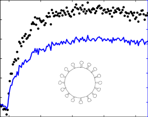
  ${\rm CO}_{2}$ concentration. The substantial increase in safe occupancy times, as one proceeds from the peak to the late stages of the pandemic, is evident in the difference between the solid and dashed lines in figure 1, which were evaluated for the case of a typical classroom in the USA (Reference Bazant and BushBazant & Bush, 2021). This example shows the critical role of exposure time in determining the safe ${\rm CO}_{2}$ level, a limit that can be increased dramatically by efficient mask use and to a lesser extent by filtration. When infection prevalence $p_i$ falls below 10 per 100 000 (an arbitrarily chosen small value), the chance of transmission is extremely low, allowing for long occupancy times. The risk of transmission at higher levels of prevalence, as may be deduced by interpolating between the solid and dashed lines in figure 1, could also be rationally managed by monitoring the ${\rm CO}_{2}$ concentration and adhering to the guideline.

Figure 1. Illustration of the safety guideline, (5), which bounds the safe excess  $\textit{CO}_{\textit{2}}$ (p.p.m.) and exposure time $\tau$ (hours). Here, we consider the case of a standard US classroom (with an area of 83.6 m2 and a ceiling height of 3.6 m) with $N=\textit{25}$ occupants, assumed to be children engaging in normal speech and light activity ( $\lambda _q s_r = \textit{30}$ quanta h $^{-1}$) with moderate risk tolerance ( $\epsilon =\textit{10 %}$). Comparison with the most restrictive bound on the indoor reproductive number without any precautions (red line) indicates that the safe $\textit{CO}_{\textit{2}}$ level or occupancy time is increased by at least an order of magnitude by the use of face masks (blue line), even with relatively inconsistent use of cloth masks ( $p_m=\textit{30 %}$). The effect of air filtration (green line) is relatively small, shown here for a case of efficient HEPA filtration ( $p_f=\textit{99 %}$) with 17 % outdoor air fraction ( $\lambda _f=\textit{5} \lambda _a$). All three bounds are increased by several orders of magnitude (dashed lines) during late pandemic conditions ( $p_ip_s=\textit{10}$ per 100 000), when it becomes increasingly unlikely to find an infected–susceptible pair in the room. The other parameters satisfy $(\lambda _v+\lambda _s)/\lambda _a=\textit{0.5}$, as could correspond to, for example, $\lambda _v=\textit{0.3}$, $\lambda _s=\textit{0.2}$ and $\lambda _a=\textit{1}$ h $^{-1}$ (1 ACH).
3. Mathematical model of ${\rm CO}_{2}$ monitoring to predict airborne disease transmission risk

3.1 $CO_{\textit{2}}$ dynamics

We follow the traditional approach of modelling gas dynamics in a well-mixed room (Reference Shair and HeitnerShair & Heitner, 1974), as a continuous stirred tank reactor (Reference Davis and DavisDavis & Davis, 2012). Given the time dependence of occupancy,  $N(t)$, mean breathing flow rate, $Q_b(t)$, and ventilation flow rate, $Q_a(t)= \lambda _a(t) V$, one may express the evolution of the excess ${\rm CO}_{2}$ concentration $C_2(t)$ in a well-mixed room through
 \begin{equation} V \frac{\textrm{d} C_2}{\textrm{d} t} = P_2(t) - Q_a(t) C_2, \end{equation}
where
 \begin{equation} P_2(t) = N(t) Q_b(t) C_{2,b} \end{equation}
is the exhaled  ${\rm CO}_{2}$ production rate. The relaxation rate for excess ${\rm CO}_{2}$ in response to changes in $P_2(t)$ is precisely equal to the ventilation rate, $\lambda _a(t) = Q_a(t)/V$. For constant $\lambda _a$, the general solution of (6) for $C_2(0)=0$ is given by
 \begin{equation} C_2(t) = \int_0^{t} \exp({-\lambda_a(t-t')}) \frac{P_2(t')}{V} \textrm{d} t', \end{equation}
which can be derived by Laplace transform or using an integrating factor. The time-averaged excess  ${\rm CO}_{2}$ concentration can be expressed as
 \begin{equation} \langle C_2 \rangle = \frac{1}{\tau}\int_0^{\tau} \left(1 - \exp({-\lambda_a(\tau-t)})\right)\frac{P_2(t)}{Q_a} \textrm{d} t \end{equation}
by switching the order of time integration. If  $P_2(t)$ is slowly varying over the ventilation time scale $\lambda _a^{-1}$, the time-averaged ${\rm CO}_{2}$ concentration may be approximated as
 \begin{equation} \langle C_2 \rangle \approx \frac{\langle P_2 \rangle}{Q_a} - \left(\frac{1-\textrm{e}^{-\lambda_a\tau}}{\lambda_a\tau}\right) \frac{P_2(\tau)}{Q_a},\end{equation}
where the excess  ${\rm CO}_{2}$ concentration approaches the ratio of the mean exhaled ${\rm CO}_{2}$ production rate to the ventilation flow rate at long times, $\tau \gg \lambda _a^{-1}$, as indicated in (4).
3.2 Infectious aerosol dynamics
Following Reference Bazant and BushBazant and Bush (Reference Bazant and Bush2021), we assume that the radius-resolved concentration of infectious aerosol-borne pathogen,  $C(r,t)$, evolves according to
 \begin{equation} V \frac{\partial C}{\partial t} = P(r,t) - \lambda_c(r,t) V C, \end{equation}
where the mean production rate,
 \begin{equation} P(r,t) = I(t)Q_b(t)n_d(r,t)V_d(r)p_m(r)c_v(r), \end{equation}
depends on the number of infected people in the room,  $I(t)$, and the size distribution $n_d(r,t)$ of exhaled droplets of volume $V_d(r)$ containing a pathogen (i.e. virion) at microscopic concentration, $c_v(r)$. The droplet size distribution is known to depend on expiratory and vocal activity (Reference Asadi, Wexler, Cappa, Barreda, Bouvier and RistenpartAsadi et al., 2019, Reference Asadi, Wexler, Cappa, Barreda, Bouvier and Ristenpart2020c; Reference Morawska, Johnson, Ristovski, Hargreaves, Mengersen, Corbett and KatoshevskiMorawska et al., 2009). Quite generally, the aerosols evolve according to a dynamic sorting process (Reference Bazant and BushBazant & Bush, 2021): the drop-size distribution evolves with time until an equilibrium distribution obtains.
Given the time evolution of excess  ${\rm CO}_{2}$ concentration, $C_2(t)$, one may deduce the radius-resolved pathogen concentration $C(r,t)$ by integrating the coupled differential equation
 \begin{equation} \frac{\partial C}{\partial t} + \lambda_c(r,t) C = \frac{P(r,t)}{P_2(t)} \left(\frac{\textrm{d} C_2}{\textrm{d} t} + \lambda_a(t) C_2 \right). \end{equation}
This integration can be done numerically or analytically via Laplace transform or integrating factors if one assumes that  $\lambda _a$, $\lambda _c$, $P$ and P 2 all vary slowly over the ventilation (air change) time scale, $\lambda _a^{-1}$. In that case, the general solution takes the form
 \begin{equation} C(r,t) \approx \frac{P}{P_2}\left(C_2(t) + (\lambda_a-\lambda_c(r)) \int_0^{t} \exp({-\lambda_c(r)(t-t')})C_2(t')\,\textrm{d} t'\right), \end{equation}
where we consider the infectious aerosol build-up from  $C(r,0)=0$.
3.3 Disease transmission dynamics
According to Markov's inequality, the probability of at least one airborne transmission taking place during the exposure time  $\tau$ is bounded above by the expected number of airborne transmissions, $T_a(\tau )$, and the two become equal in the (typical) limit of rare transmissions, $T_a(\tau )\ll 1$. The expected number of transmissions to $S(t)$ susceptible people is obtained by integrating the mask-filtered inhalation rate of infection quanta over both droplet radius and time:
 \begin{equation} T_a(\tau) = \int_0^{\tau} S(t) Q_b(t) s_r \left( \int_0^{\infty} C(r,t) c_i(r) p_m(r)\,\textrm{d} r \right)\textrm{d} t , \end{equation}
where  $c_i(r)$ is the infectivity of the aerosolized pathogen. The infectivity is measured in units of infection quanta per pathogen and generally depends on droplet size. One might expect pathogens contained in smaller aerosol droplets with $r < 5\ \mathrm {\mu }$m to be more infectious than those in larger drops, as reported by Reference Santarpia, Herrera, Rivera, Ratnesar-Shumate, Reid, Denton and LoweSantarpia et al. (Reference Santarpia, Herrera, Rivera, Ratnesar-Shumate, Reid, Denton and Lowe2020) for SARS-CoV-2, on the grounds that smaller drops more easily penetrate the respiratory tract, absorb and coalesce onto exposed tissues, and allow pathogens to escape more quickly by diffusion to infect target cells. The mask penetration probability $p_m(r)$ also decreases rapidly with increasing drop size above the aerosol range for most filtration materials (Reference Chen and WillekeChen & Willeke, 1992; Reference Konda, Prakash, Moss, Schmoldt, Grant and GuhaKonda et al., 2020b; Reference Li, Guo, Wong, Chung, Gohel and LeungLi et al., 2008; Reference Oberg and BrosseauOberg & Brosseau, 2008), so the integration over all radii in (15) gives the most weight to the aerosol size range, roughly $r < 5\ \mathrm {\mu }$m. We note that this range includes the maxima in exhaled droplet size distributions (Reference Asadi, Wexler, Cappa, Barreda, Bouvier and RistenpartAsadi et al., 2019, Reference Asadi, Wexler, Cappa, Barreda, Bouvier and Ristenpart2020c; Reference Morawska, Johnson, Ristovski, Hargreaves, Mengersen, Corbett and KatoshevskiMorawska et al., 2009) as defined in terms of either number or total volume in the aerosol range (Reference Bazant and BushBazant & Bush, 2021); nevertheless, larger droplets may also contribute to airborne transmission (Reference Tang, Bahnfleth, Bluyssen, Buonanno, Jimenez, Kurnitski and DancerTang et al., 2021).
The inverse of the infectivity,  $c_i^{-1}$, is equal to the ‘infectious dose’ of pathogens from inhaled aerosol droplets that would cause infection with probability $1-(1/e)=63\,\%$. Reference Bazant and BushBazant and Bush (Reference Bazant and Bush2021) estimated the infectious dose for SARS-CoV-2 to be of the order of 10 aerosol-borne virions. Notably, the corresponding infectivity, $c_i \sim 0.1$, is an order of magnitude larger than previous estimates for SARS-CoV (Reference Buonanno, Stabile and MorawskaBuonanno et al., 2020b; Reference Watanabe, Bartrand, Weir, Omura and HaasWatanabe, Bartrand, Weir, Omura & Haas, 2010), which is consistent with only COVID-19 reaching pandemic status. The infectivity is known to vary across different age groups and pathogen strains, a variability that is captured by the relative susceptibility, $s_r$. For example, Reference Bazant and BushBazant and Bush (Reference Bazant and Bush2021) suggest assigning $s_r=1$ for the elderly (over 65 years old), $s_r=0.68$ for adults (aged 15–64) and $s_r=0.23$ for children (aged 0–14) for the original Wuhan strain of SARS-CoV-2, based on a study of transmission in quarantined households in China (Reference Zhang, Litvinova, Liang, Wang, Wang, Zhao and YuZhang et al., 2020a). The authors further suggested multiplying these values by $1.6$ for the more infectious Alpha variant of concern of the lineage B.1.1.7 (VOC 202012/01), which emerged in the UK with a reproductive number that was 60 % larger than that of the original strain (Reference Davies, Barnard, Jarvis, Kucharski, Munday, Pearson and EdmundsDavies et al., 2020; Reference Volz, Mishra, Chand, Barrett, Johnson, Geidelberg and FergusonVolz et al., 2021). Based on the latest epidemiological data (Reference Abdool Karim and de OliveiraAbdool Karim & de Oliveira, 2021), we likewise suggest multiplying $s_r$ by $1.5$ for the South African variant, 501 Y.V2, and by $1.2$ for the Californian variants, B.1.427 and B.1.429. Appropriate factors multiplying sr for more recent strains are provided on our online app (Reference Khan, Bazant and BushKhan, Bazant & Bush, 2020), such as 1.5 for the Beta variant B.1.351 from South Africa, 2.0 for the Gamma variant P.1 from Brazil and 2.5 for the Delta variant B.1.617.2 from India that has become dominant at the time of publication.
3.4 Approximate formula for the airborne transmission risk from $CO_{\textit{2}}$ measurements

Equations (14) and (15) provide an approximate solution to the full model that depends on the exhaled droplet size distribution,  $n_d(r,t)$, and mean breathing rate, $Q_b(t)$, of the population in the room. Since the droplet distributions $n_d(r)$ have only been characterized in certain idealized experimental conditions (Reference Asadi, Bouvier, Wexler and RistenpartAsadi et al., 2020a, Reference Asadi, Wexler, Cappa, Barreda, Bouvier and Ristenpart2020c; Reference Morawska, Johnson, Ristovski, Hargreaves, Mengersen, Corbett and KatoshevskiMorawska et al., 2009), it is useful to integrate over $r$ to obtain a simpler model that can be directly calibrated for different modes of respiration using epidemiological data (Reference Bazant and BushBazant & Bush, 2021). Assuming $Q_b(t)$, $I(t)$, $S(t)$, $N(t)$ and $n_d(r,t)$ vary slowly over the relaxation time $\overline {\lambda }_c^{-1}$, we may substitute (14) into (15) and perform the time integral of the second term to obtain
 \begin{align} T_a(\tau) \approx \frac{s_r \lambda_a}{C_{2,b}} \int_0^{\tau} \int_0^{\infty} \frac{n_q(r,t)p_m(r)^{2}}{\lambda_c(r)} \frac{Q_b(t) I(t) S(t) C_2(t)}{N(t)} \left[ 1 + \left(\frac{\lambda_c(r)}{\lambda_a} - 1 \right) \exp({-\lambda_c(r)(\tau-t)})\right]\textrm{d} r\,\textrm{d} t, \end{align}
where  $n_q(r,t)=n_d(r,t)V_d(r)c_v(r)c_i(r)$ is the radius-resolved exhaled quanta concentration.
Following Reference Bazant and BushBazant and Bush (Reference Bazant and Bush2021), we define an effective radius of infectious aerosols  $\overline {r}$ such that
 \begin{equation} \int_0^{\infty} \frac{n_q(r,t) p_m(r)^{2}}{\lambda_c(r)} \textrm{d} r \equiv \frac{C_q(t) p_m(\overline{r})^{2}}{\lambda_c(\overline{r})},\end{equation}
where  $C_q(t) = \int _0^{\infty } n_q(r,t)\,\textrm {d} r$ is the exhaled quanta concentration, which may vary in time with changes in expiratory activity, for example, following a transition from nose breathing to speaking. In principle, the effective radius $\overline {r}$ can be evaluated, given a complete knowledge of the dependence on drop radius of the mask penetration probability, $p_m(r)$, and of all the factors that determine the exhaled quanta concentration, $n_q(r,t)$ and pathogen removal rate, $\lambda _c(r)$. While these dependencies are not readily characterized, typical values of $\overline {r}$ are at the scale of several microns, based on the size dependencies of $n_d(r,t)$, $c_i(r)$ and $p_m(r)$ noted above.
Further simplifications allow us to derive a formula relating  ${\rm CO}_{2}$ measurements to transmission risk. By assuming that $C_q(t)$ varies slowly over the time scale of concentration relaxation, one may approximate the memory integral with the same effective radius $\overline {r}$. Thus, accounting for immunity and infection prevalence in the population via
 \begin{equation} \frac{I(t) S(t)}{N(t)} \approx \frac{N_t}{N} = \left(1 - \frac{1}{N}\right) \min\{1,Np_ip_s\}, \end{equation}
we obtain a formula for the expected number of airborne transmissions,
 \begin{equation} T_a(\tau) \approx \frac{s_r \overline{p}_m^{2}}{C_{2,b}} \frac{\lambda_a}{\overline{\lambda}_c} \frac{N_t}{N} \int_0^{\tau} \lambda_q(t) C_2(t)\left[ 1 + \left(\frac{\overline{\lambda}_c}{\lambda_a} - 1\right) \exp({-\overline{\lambda}_c(\tau-t)})\right]\textrm{d} t, \end{equation}
in terms of the excess  ${\rm CO}_{2}$ time series, $C_2(t)$, where $\lambda _q(t)=C_q(t)Q_b(t)$ is the mean quanta emission rate. It is also useful to define the expected transmission rate,
 \begin{align} \frac{\textrm{d} T_a}{\textrm{d} t}(\tau) = N_t \beta_a(\tau) = \frac{s_r \overline{p}_m^{2}}{C_{2,b}} \frac{\lambda_a}{\overline{\lambda}_c} \frac{N_t}{N} \left[\lambda_q(\tau) C_2(\tau) + (\lambda_a - \overline{\lambda}_c) \int_0^{\tau} \lambda_q(t)C_2(t) \exp({-\overline{\lambda}_c(\tau-t)})\,\textrm{d} t\right], \end{align}
which allows for direct assessment of airborne transmission risk based on  ${\rm CO}_{2}$ levels. A pair of examples of such assessments will be presented in § 4.
Notably, the mean airborne transmission rate expected per infected–susceptible pair,  $\beta _a(t)$, reflects the environment's memory of the recent past, which persists over the pathogen relaxation time scale, $\overline {\lambda }_c^{-1}$. Likewise, the ${\rm CO}_{2}$ concentration defined in (9) has a memory of recent changes in ${\rm CO}_{2}$ sources or ventilation, which persists over the air change time scale. Notably, the airborne pathogen concentration equilibrates more rapidly than CO $_2$; specifically, $\lambda _a^{-1} > \overline {\lambda }_c^{-1}$, since ${\rm CO}_{2}$ is unaffected by the filtration, sedimentation and deactivation rates enumerated in (2). The time delays between the production of ${\rm CO}_{2}$ and infectious aerosols by exhalation and their build-up in the well-mixed air of a room shows that ${\rm CO}_{2}$ variation and airborne transmission are inherently non-Markovian stochastic processes. As such, any attempt to predict fluctuations in airborne transmission risk would require stochastic generalizations of the differential equations governing the mean variables, (6) and (11), and so represent a stochastic formulation of the Wells–Riley model (Reference Noakes and SleighNoakes & Sleigh, 2009).
3.5 Reduction to the $CO_{\textit{2}}$-based safety guideline

Finally, we connect the general result, (19), with the  ${\rm CO}_{2}$-based safety guideline derived above, (5). Since $C_2(t)$ varies on the ventilation time scale $\lambda _a^{-1}$, which is necessarily longer than the relaxation time scale of the infectious aerosols $\overline {\lambda }_c^{-1}$, we may assume that $\lambda _q(t)C_2(t)$ is slowly varying and evaluate the integral in (19). We thus arrive at the approximation
 \begin{equation} T_a(\tau) \approx \frac{s_r \overline{p}_m^{2}}{C_{2,b}} \frac{\lambda_a}{\overline{\lambda}_c} \frac{N_t}{N} \left[\langle \lambda_q C_2 \rangle \tau + \frac{\lambda_q(\tau)C_2(\tau)}{\overline{\lambda}_c} \left(\frac{\overline{\lambda}_c}{\lambda_a}-1 + \textrm{e}^{-\overline{\lambda}_c\tau} \right) \right]. \end{equation}
Since  $\lambda _q(t)C_2(t)$ is slowly varying, the second term in brackets is negligible relative to the first for times longer than the ventilation time, $\tau \gg \lambda _a^{-1} > \overline {\lambda }_c^{-1}$. In this limit, the imposed bound on expected transmissions, $T_a(\tau ) < \epsilon$, is approximated by
 \begin{equation} \langle \lambda_q C_2 \rangle \tau = \int_0^{\tau} \lambda_q(t)C_2(t)\,\textrm{d} t < \frac{\epsilon C_{2,b}}{s_r \overline{p}_m^{2}} \frac{\overline{\lambda}_c}{\lambda_a} \frac{N}{N_t}.\end{equation}
This formula reduces to the safety guideline, (5), in the limit of constant mean quanta emission rate,  $\lambda _q$, which confirms the consistency of our assumptions.
4. Examples of implementation
We proceed by illustrating the process by which the guideline, (5), can be coupled to real data obtained from  ${\rm CO}_{2}$ monitors. Specifically, we consider time series of ${\rm CO}_{2}$ concentration gathered in classroom and office settings at the Massachusetts Institute of Technology using an Atlas Scientific EZO-CO2 Embedded NDIR CO2 Sensor controlled with an Arduino Uno and an Aranet4, respectively. The measurements were collected at desk level. Social distancing guidelines were adhered to, and masks were worn by all participants. We assume a constant exhaled ${\rm CO}_{2}$ concentration of 38 000 p.p.m., and use the global minimum of the ${\rm CO}_{2}$ series as the background ${\rm CO}_{2}$ level $C_0$ from which the excess concentration $C_2(t)$ was deduced. Notably, the relatively small fluctuations in the ${\rm CO}_{2}$ measurements recorded in a variety of settings support the notion of a well-mixed room.
The sensors yield a time series of CO $_2$ concentration that we use, along with (19) and (20), to calculate the transmission rate, assuming that there is a single infected person in the room and that all others are susceptible ( $N_t = N-1$). In this case, the expected number of transmissions is equal to the indoor reproductive number, $T_a(\tau ) = \mathcal {R}_{\textrm {in}}(\tau )$, and the transmission rate is $({\textrm {d} T_a}/{\textrm {d} t})(\tau ) = N_t \beta _a(\tau )$. The approximations made in the derivation above are valid in these examples, so a direct numerical solution of (13) would yield an identical result. In particular, the ‘slowly varying’ assumptions are satisfied, since we keep $N$ and $I$ constant, and any time-dependence of $Q_b$ cancels in the ratio $P/P_2$. Moreover, there was no indication that the air change rate varied over the relatively short time periods considered. Finally, the droplet distributions $n_d(r,t)$ may vary in time, but no significant changes in mean respiratory activity were observed or evidenced in the CO $_2$ measurements.
We choose realistic values of the parameters that fall within the typical ranges estimated by Reference Bazant and BushBazant and Bush (Reference Bazant and Bush2021). The mean breathing rate is set to a value,  $Q_b=0.5$ m $^{3}$ h $^{-1}$, appropriate for light respiratory activity, and we choose an effective settling speed of $\overline {v}_s=0.108$ m h $^{-1}$ appropriate for $\bar {r}=0.5\ \mathrm {\mu }$m. Larger values of $Q_b$ would be appropriate for more vigorous respiratory activity, as would accompany, for example, a workout at a gym. Our estimate for $\overline {v}_s$ may be revised in response to additional information concerning the dependence on size of the infectivity of exhaled aerosol droplets (Reference Stadnytskyi, Bax, Bax and AnfinrudStadnytskyi et al., 2020). The viral deactivation rate for SARS-CoV-2 is set to $\lambda _v = 0.3$ h $^{-1}$, an estimate appropriate for 50 % relative humidity. We plot $N_t \beta _a(\tau )$ and $\mathcal {R}_{\textrm {in}}(\tau )$ for cases where masks are and are not worn, and choose a mask penetration probability of $p_m \approx 0.3$, as is roughly appropriate for a cloth mask (Reference Konda, Prakash, Moss, Schmoldt, Grant and GuhaKonda et al., 2020a). For more effective masks, such as surgical masks or N95s, a smaller $p_m$ value is appropriate, as noted above. The parameters $\overline {\lambda }_c$, $\lambda _a$, $H$ and $N$ are chosen according to the specific scenario presented. Exhaled COVID-19 quanta concentrations $C_q$ for various expiratory activities are estimated from figure 2 of Reference Bazant and BushBazant and Bush (Reference Bazant and Bush2021). In order to be conservative, we assume that $s_r=1$, suitable for the most susceptible individuals exposed to the Wuhan strain of SARS-CoV-2. When applying our model to less susceptible populations, such as children (Reference Zhang, Litvinova, Liang, Wang, Wang, Zhao and YuZhang et al., 2020a; Reference Zhu, Bloxham, Hulme, Sinclair, Tong, Steele and ShortZhu et al., 2020) or vaccinated individuals exposed to new variants (Reference Sheikh, McMenamin, Taylor and RobertsonSheikh et al., 2021; Reference Nasreen, He, Chung, Brown, Gubbay, Buchan and KwongNasreen et al., 2021), a smaller $s_r$ value may be used.
4.1 Small office with two workers
Figure 2a shows  $\text{CO}_{2}$ measurements taken in an office of length $L = 4.2$ m, width $W = 3$ m and height $H = 3$ m. Initially, a single worker is present, but at 19:00, a second worker arrives at the office. The workers exit the office at 21:09, return at 21:39 and exit again at 22:30. As the participants were speaking, we use $C_q=72$ quanta m $^{-3}$ (Reference Bazant and BushBazant & Bush, 2021). We compute the room's ventilation rate, $\lambda _a \approx 2.3\ {\rm h}^{-1}$, from the exponential relaxation that follows the occupants’ exit from the office (as indicated by the orange curve in figure 2). The office was equipped with moderate ventilation, which we characterize with $p_f=0.99$ and $\lambda _r = 6$ h $^{-1}$. The background concentration $C_0 = 420$ p.p.m. is evident both before and after occupancy.

Figure 2. Measured  $\textit{CO}_{2}$ concentration and calculated transmission rate in a two-person office. (a) Black dots represent the concentration of $\textit{CO}_{2}$. The solid blue, dashed magenta and dash–dot green curves represents the transmission rate, as calculated from (20) for three different scenarios, two of which were hypothetical: (blue) the pair are not wearing masks and there is no filtration present; (magenta) the pair are not wearing masks and there is filtration present; (green) the pair are wearing masks and there is no filtration present. The orange solid curve denotes the period of exponential relaxation following the exit of the room's occupants, from which one may infer both the room's ventilation rate, $\lambda _a = \textit{2.3}$ h $^{-1}$, and the background CO $_2$ concentration, $C_0 = \textit{420}$ p.p.m. (b) Corresponding blue, magenta and green curves, deduced by integrating (20), indicate the total risk of transmission over the time of shared occupancy. If the pair were not wearing masks, the safety limit $\mathcal {R}_{\textrm {in}} < \textit{0.1}$ would be violated after approximately an hour.
As shown in figure 2b, if the office workers were not wearing masks, the safety guideline of expected transmissions  $T_a < 10\,\%$ would be violated after approximately an hour together. However, office workers wearing cloth masks would not violate the safety guideline during the 2.5 h spent together. Filtration without masks also extends the occupancy time limits; however, $\mathcal {R}_{\textrm {in}}$ approaches the safety limit after approximately 2 h. While this example should not be taken as a definitive statement of danger or safety in this setting, it does serves to illustrate how our ${\rm CO}_{2}$ guideline can be implemented in a real-life situation.
4.2 University classroom adhering to social distancing guidelines
We next monitor  ${\rm CO}_{2}$ levels during a university lecture. There were $N=12$ participants in a lecture hall of length $L = 13$ m, width $W = 12$ m and height $H = 3$ m. The lecture started at 13:05 and finished at 13:50. Four people remained in the room for 30 min after the class. The classroom has mechanical ventilation, which is characterized in terms of $\lambda _a \approx 5.2$ h $^{-1}$ (corresponding to a 12 min outdoor air change time; here, we estimate $\lambda _a$ by fitting the build-up of ${\rm CO}_{2}$, see figure 3). During the lecture, the professor spoke while the students were quiet and sedentary; thus, we assume $C_q = 30$ quanta m $^{-3}$ (Reference Bazant and BushBazant & Bush, 2021). The maximum ${\rm CO}_{2}$ concentration reached in the classroom was ${\approx }550$ p.p.m., the excess level no more than 100 p.p.m. Thus, the safety limit was never exceeded, and would not have been even if masks had not been worn. We note that this lecture hall was particularly large, well-ventilated and sparsely populated, and so should not be taken as being representative of a classroom setting. A more complete assessment of safety in schools would require integrating ${\rm CO}_{2}$ concentrations over a considerably longer time interval. For example, if students are tested weekly for COVID-19, then one should assess the mean ${\rm CO}_{2}$ concentration in class during the course of an entire school week. Nevertheless, this second example further illustrates the manner in which our model may be applied to real-world settings and suggests that precautions such as ventilation, filtration and mask use, can substantially increase safe occupancy times.

Figure 3. Measured  $\textit{CO}_{\textit{2}}$ concentration and calculated transmission rate for 12 masked students in a university lecture hall. (a) Black dots represent the concentration of $\textit{CO}_{\textit{2}}$. The dash–dot green and solid blue curves represent the transmission rate, as calculated from (20), when the occupants are wearing masks, and in the hypothetical case where they are not, respectively. The gold curve indicates a fit to the transient build-up of $\textit{CO}_{\textit{2}}$ from which we infer an air change rate of $\lambda _a = \textit{5.2}/h$. (b) The dash–dot green and solid blue curves indicate the total risk of transmission with and without masks, respectively, as deduced by integrating (20) over time. Even had masks not been worn, the safety guideline would not have been violated during the lecture.
5. Conclusion
Mounting evidence suggests that COVID-19 is spread primarily via indoor airborne transmission. Such an inference is no surprise, as such is also the case for many other respiratory illnesses, including influenza, tuberculosis, measles and severe acute respiratory syndrome (as is caused by a precursor to SARS-CoV-2, the coronavirus SARS-CoV). More than a year into the pandemic, public health guidance continues to emphasize the importance of social distancing and surface cleaning, despite evidence that mask directives are much more effective than either in limiting airborne transmission. We have here illustrated the manner in which  ${\rm CO}_{2}$ monitoring may be used in conjunction with the safety guideline of Reference Bazant and BushBazant and Bush (Reference Bazant and Bush2021) to assess the risk of indoor airborne respiratory disease transmission, including that of COVID-19. Reference Morawska, Allen, Bahnfleth, Bluyssen, Boerstra, Buonanno and YaoMorawska et al. (Reference Morawska, Allen, Bahnfleth, Bluyssen, Boerstra, Buonanno and Yao2021) emphasize the need for improved air quality standards to combat airborne respiratory diseases, similar in spirit to food safety standards for restaurants. We hope that our study might prove useful in defining such standards, and in informing personal and policy decisions about closing and reopening indoor spaces, such as schools and businesses.
We have here reformulated the COVID-19 indoor safety guideline of Reference Bazant and BushBazant and Bush (Reference Bazant and Bush2021), expressing it in terms of cumulative exposure to  ${\rm CO}_{2}$, which can be readily monitored in real time for most indoor spaces. In so doing, we have built upon the seminal work of Reference Rudnick and MiltonRudnick and Milton (Reference Rudnick and Milton2003), as was recently extended and applied to COVID-19 by Reference Peng and JimenezPeng and Jimenez (Reference Peng and Jimenez2021). The guideline of Reference Bazant and BushBazant and Bush (Reference Bazant and Bush2021) makes clear that, since the risk of indoor airborne infection is determined by the total volume of pathogen inhaled, safety limits intended to protect against it must be expressed in terms of occupancy time. Likewise, in the context of CO $_2$ measurements, safety limits cannot be expressed solely in terms of a limit on ${\rm CO}_{2}$ levels, but must also depend on occupancy time. As we have demonstrated with our two case studies, the safety guideline, (5), when coupled with CO $_2$ monitors, allows for real-time assessment of risk of airborne disease transmission $\mathcal {R}_{\textrm {in}}$ in indoor spaces. Moreover, this approach has the distinct advantage that one can assess certain key model parameters, including the background concentration of CO $_2$ and the room's ventilation rate, directly from the CO $_2$ measurements.
Within a well-mixed space,  ${\rm CO}_{2}$ is effectively a passive scalar that tracks the ambient flow, and is removed only through exchange with outdoor air. Aerosol-borne pathogens are subject to additional removal mechanisms, including filtration (by face masks and internal circulation), sedimentation and deactivation. Thus, the concentration of CO $_2$ cannot be taken as a proxy for those of an aerosol-borne pathogen without resolving the proportionality constant between the two that results from these additional removal mechanisms. We stress that the effects of face mask use are dramatic in reducing the ratio of aerosol-borne pathogens to CO $_2$ concentration, and in reducing the risk of indoor transmission. Finally, we note that the additional removal mechanisms acting on the droplet-borne pathogen alter not only its equilibrium concentrations relative to that of CO $_2$, but their relaxation times in transient situations, as may be treated using the mathematical formalism of Reference Bazant and BushBazant and Bush (Reference Bazant and Bush2021).
We emphasize that the caveats enumerated by Reference Bazant and BushBazant and Bush (Reference Bazant and Bush2021) concerning the limitations of their safety guideline apply similarly here. First, there is considerable uncertainty in a number of model parameters, including the critical viral load and relative susceptibility. While our inferences are consistent with available data, we hope that these uncertainties will be reduced as more COVID-19 spreading events are characterized and analysed. Second, when masks are not worn, there is substantial additional risk of short-range airborne transmission from respiratory jets and plumes, as accompany breathing, speaking (Reference Abkarian, Mendez, Xue, Yang and StoneAbkarian et al., 2020a; Reference Abkarian and StoneAbkarian & Stone, 2020), coughing and sneezing (Reference Bourouiba, Dehandschoewercker and BushBourouiba et al., 2014). Third, while the assumption of the well-mixed room is widely applied and represents a reasonable first approximation, it is known to have limitations (Reference Bhagat, Wykes, Dalziel and LindenBhagat et al., 2020; Reference Linden, Lane-Serff and SmeedLinden, Lane-Serff & Smeed, 1990; Reference LindenLinden, 1999). Notably, measured fluctuations in  ${\rm CO}_{2}$ levels provide a direct means of assessing the validity of the well-mixed-room hypothesis, especially when several sensors are used simultaneously at different locations in the same space. Indeed, ${\rm CO}_{2}$ monitoring has been used for decades to assess the quality of air handling and zonal mixing in buildings (Reference Cheng, Acevedo-Bolton, Jiang, Klepeis, Ott, Fringer and HildemannCheng et al., 2011; Reference Fisk and De AlmeidaFisk & De Almeida, 1998; Reference Hung and DerossisHung & Derossis, 1989; Reference SalisburySalisbury, 1986; Reference Seppänen, Fisk and MendellSeppänen et al., 1999), and can now be repurposed to assess the risk of indoor airborne disease transmission.
Our transmission theory and safety guideline provide a quantitative basis for the use of  ${\rm CO}_{2}$ monitors in assessing the risk of indoor airborne disease transmission. Specifically, the simple guideline, (5), and mathematical formulae connecting ${\rm CO}_{2}$ data to the evolving transmission risk, (19)–(20), pave the way for real-time assessment of personal risk in indoor spaces. Our safety guideline might also be implemented in spaces where not only ${\rm CO}_{2}$ is monitored, but also other relevant model parameters. For example, changes in occupancy could be monitored at entrances and exits, while monitoring decibel levels and type of vocalization would serve to inform the infectious aerosol production rate (Reference Asadi, Wexler, Cappa, Barreda, Bouvier and RistenpartAsadi et al., 2019, Reference Asadi, Wexler, Cappa, Barreda, Bouvier and Ristenpart2020c; Reference Morawska, Johnson, Ristovski, Hargreaves, Mengersen, Corbett and KatoshevskiMorawska et al., 2009). One could further envision feeding all such data into air regulation controls in order to ensure that our ${\rm CO}_{2}$-based indoor safety limit is never violated. We note that such a prospect would be most easily achieved in quasi-steady circumstances in which a fixed population is behaving in a predictable fashion over the course of an event of known duration, for example, students in a lecture hall or passengers on a charter bus. In more complicated situations, our model provides a framework for optimizing sensor-based, demand-controlled ventilation (Reference Fisk and De AlmeidaFisk & De Almeida, 1998), with a view to limiting transmission risk while reducing energy consumption and system costs (Reference Risbeck, Bazant, Jiang, Lee, Drees and DouglasRisbeck et al. 2021a, Reference Risbeck, Bazant, Jiang, Lee, Drees and Douglas2021b). Finally, our model provides a general framework for using ${\rm CO}_{2}$ monitors to mitigate the indoor airborne transmission of other respiratory illnesses, including the seasonal flu.
In order to facilitate the application of our safety guideline, in the supplementary material we provide a link to an online app that computes the safety guideline in terms of both room occupancy and  ${\rm CO}_{2}$ levels (Reference Khan, Bazant and BushKhan et al., 2020). The ${\rm CO}_{2}$-based guideline, available in the app's advanced mode, may be used in conjunction with ${\rm CO}_{2}$ monitors to formulate safe reopening strategies for indoor spaces in the later stages of the pandemic.
Acknowledgements
We thank L. Champion for valuable discussions and for sharing preliminary data and Roberto Rondanelli for references.
Funding Statement
The authors received no funding for this work.
Declaration of Interests
The authors report no conflict of interest.
Data Availability Statement
Raw data are available from M.Z.B. and O.K.
Ethical Standards
The research meets all ethical guidelines, including adherence to the legal requirements of the study country.
Supplementary Material
Supplementary material are available at https://indoor-covid-safety.herokuapp.com.


 Open access