


Introduction
One important parameter that affects the driving cycles in a city is its traffic condition. Besides influencing driving behavior (Balsa-Barreiro et al., Reference Balsa-Barreiro, Valero-Mora, Menendez and Mehmood2020), it also has an impact on the emission, energy, and fuel consumption of the vehicle (Gebisa et al., Reference Gebisa, Gebresenbet, Gopal and Nallamothu2021; Lejri et al., Reference Lejri, Can, Schiper and Leclercq2018). Therefore, when engineers tend to develop a driving cycle for a city, the traffic condition must be considered during data acquisition.
In an urban environment, traffic congestion is dependent on the time and the route. If we take the time parameter, as expected, heavier traffic can usually be seen during weekdays and at peak times, while lighter traffic can be observed during weekends and public holidays (Abas et al., Reference Abas, Rajoo and Abidin2018). If analyzing the effect of routes, the traffic flow will be influenced by the topography, the road type, the density of population and business centers, weather conditions, etc.
In this regard, Fotouhi and Montazeri-Gh (Reference Fotouhi and Montazeri-Gh2013) developed the Tehran (Iran) driving cycle by the K-means clustering approach. They clustered the driving data based on four traffic congestion types, namely congested, urban, extra-urban, and highway driving, based on the vehicle speeds. Chugh et al. (Reference Chugh, Kumar, Muralidharan, Kumar, Sithananthan, Gupta, Basu and Malhotra2012) extracted the Delhi (India) driving cycle based on monitoring the traffic conditions for three days. They also categorized traffic into congested, semi-urban, urban, and extra-urban. Pouresmaeili et al. (Reference Pouresmaeili, Aghayan and Taghizadeh2018) used the hourly measurements of air pollutant stations to find the traffic condition in the city of Mashhad. The peaks were in the morning (7:00) and in the afternoon (16:00), based on the concentration of air pollutants.
In this dataset, the traffic conditions were considered for data acquisition of driving cycles by passenger cars in Semnan city.
Data description
After covering a distance of 670 km and driving for 13 hours over 7 days, the Global Positioning System (GPS) data were collected. More information about the process of data logging is provided in the section on Experimental design, materials, and methods. There were 96 unique data in the repository that each included three files with different file extensions. Tables 1–7 and 8–14 list the data for characteristics of driving cycles of the Toyota Prius and the Peugeot Pars (or the IKCO Persia), respectively. Note that each one was identical and there were no changes implemented during the process of data logging.
Table 1. Characteristics of logged data on Thursday, July 21, 2022, for the Prius
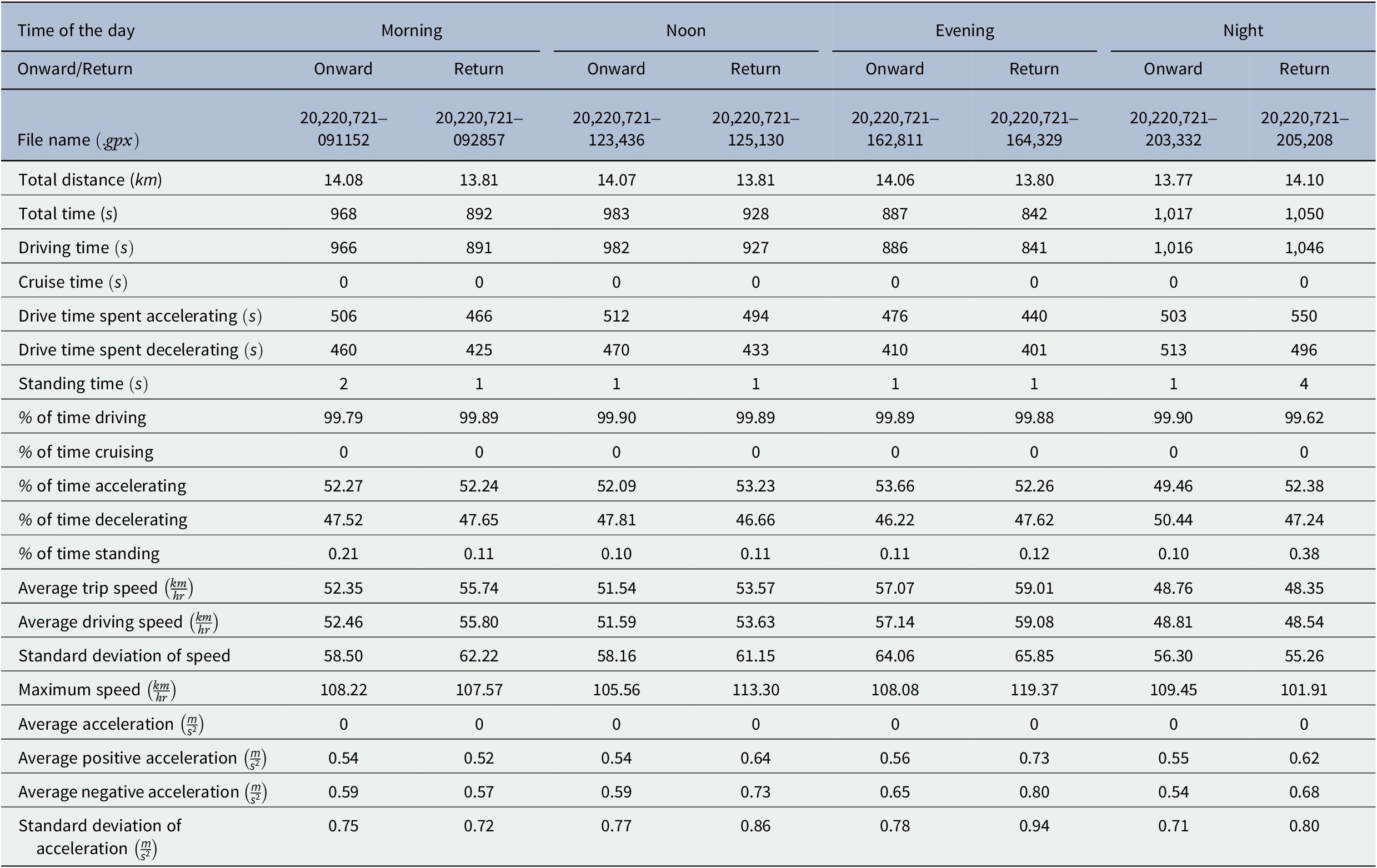
Table 2. Characteristics of logged data on Friday, July 22, 2022, for the Prius
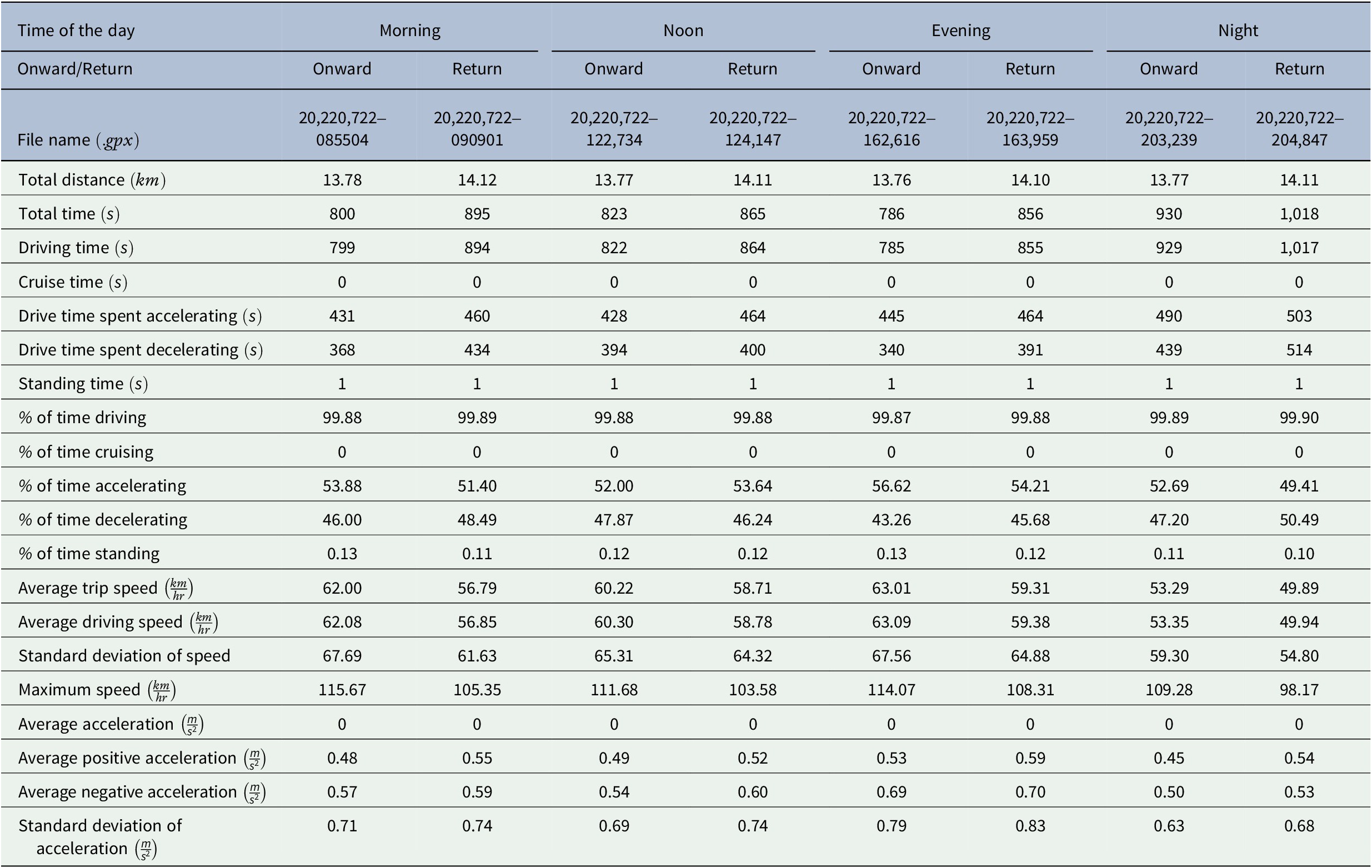
Table 3. Characteristics of logged data on Saturday, July 23, 2022, for the Prius
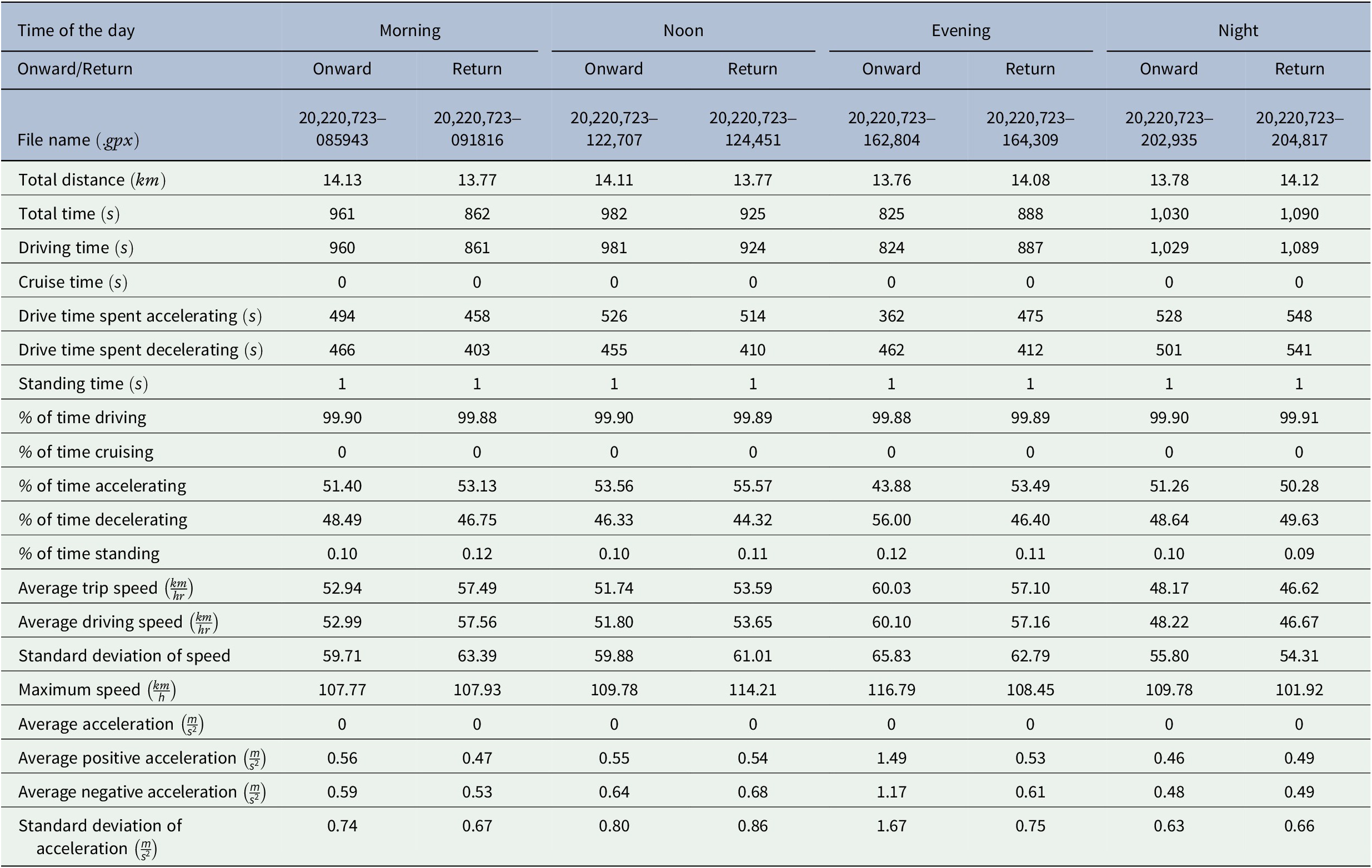
Table 4. Characteristics of logged data on Sunday, July 24, 2022, for the Prius
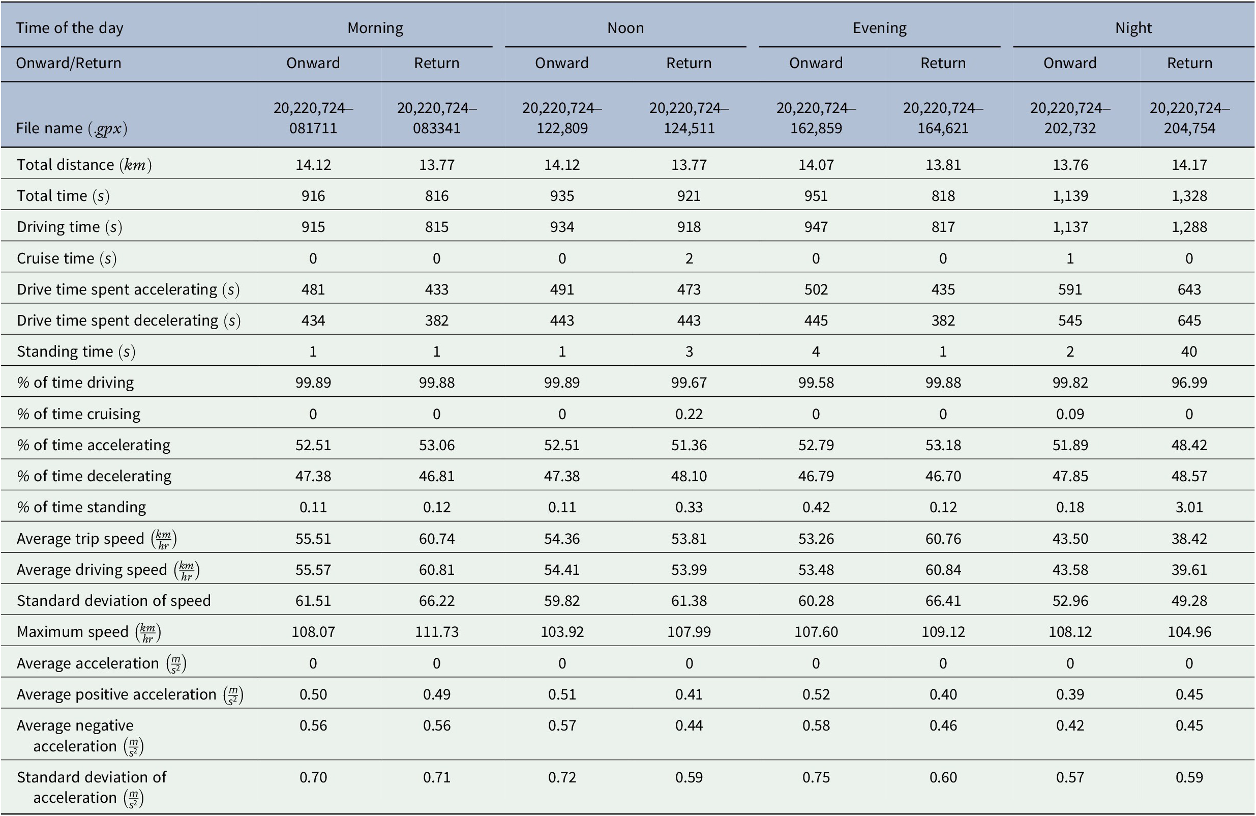
Table 5. Characteristics of logged data on Monday, July 25, 2022, for the Prius
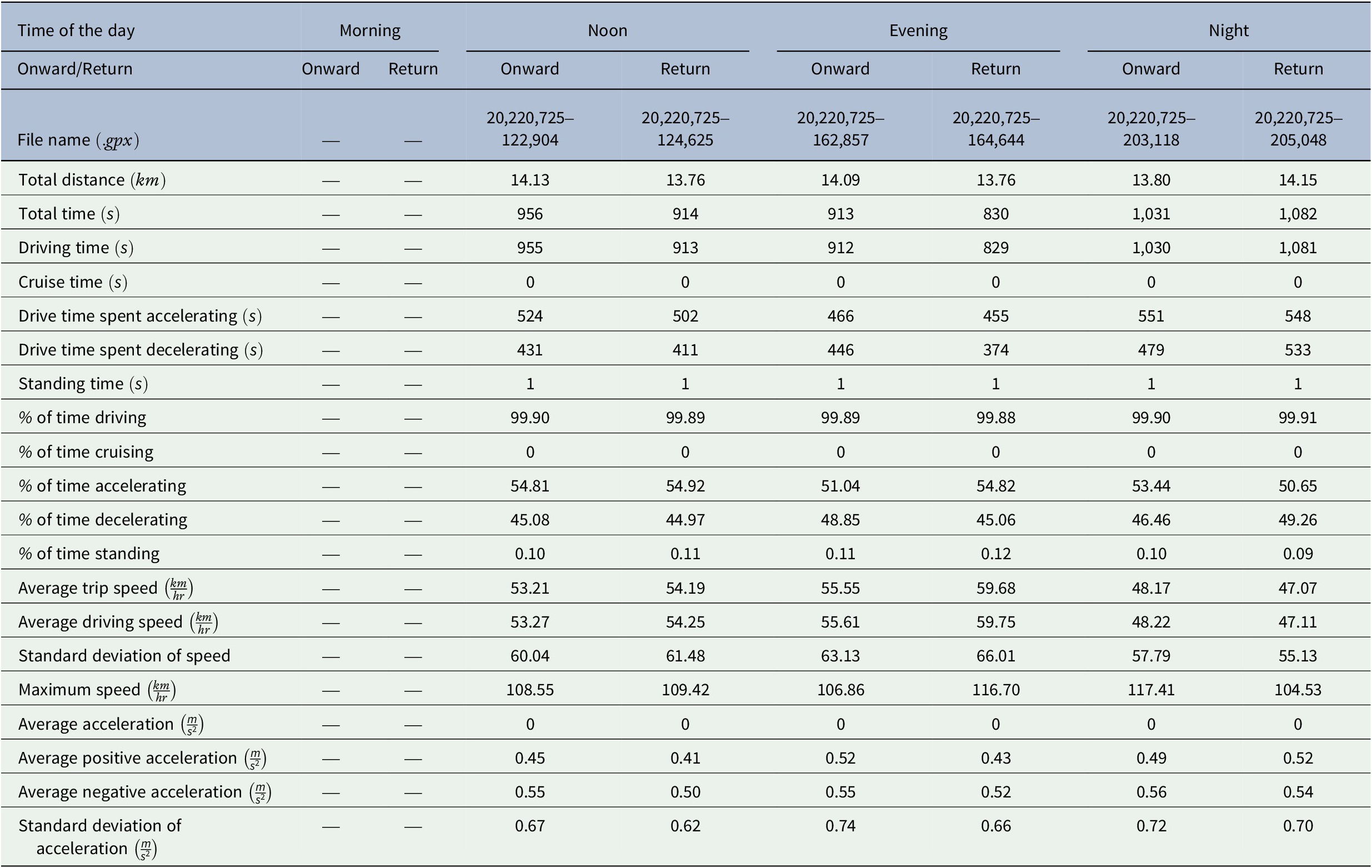
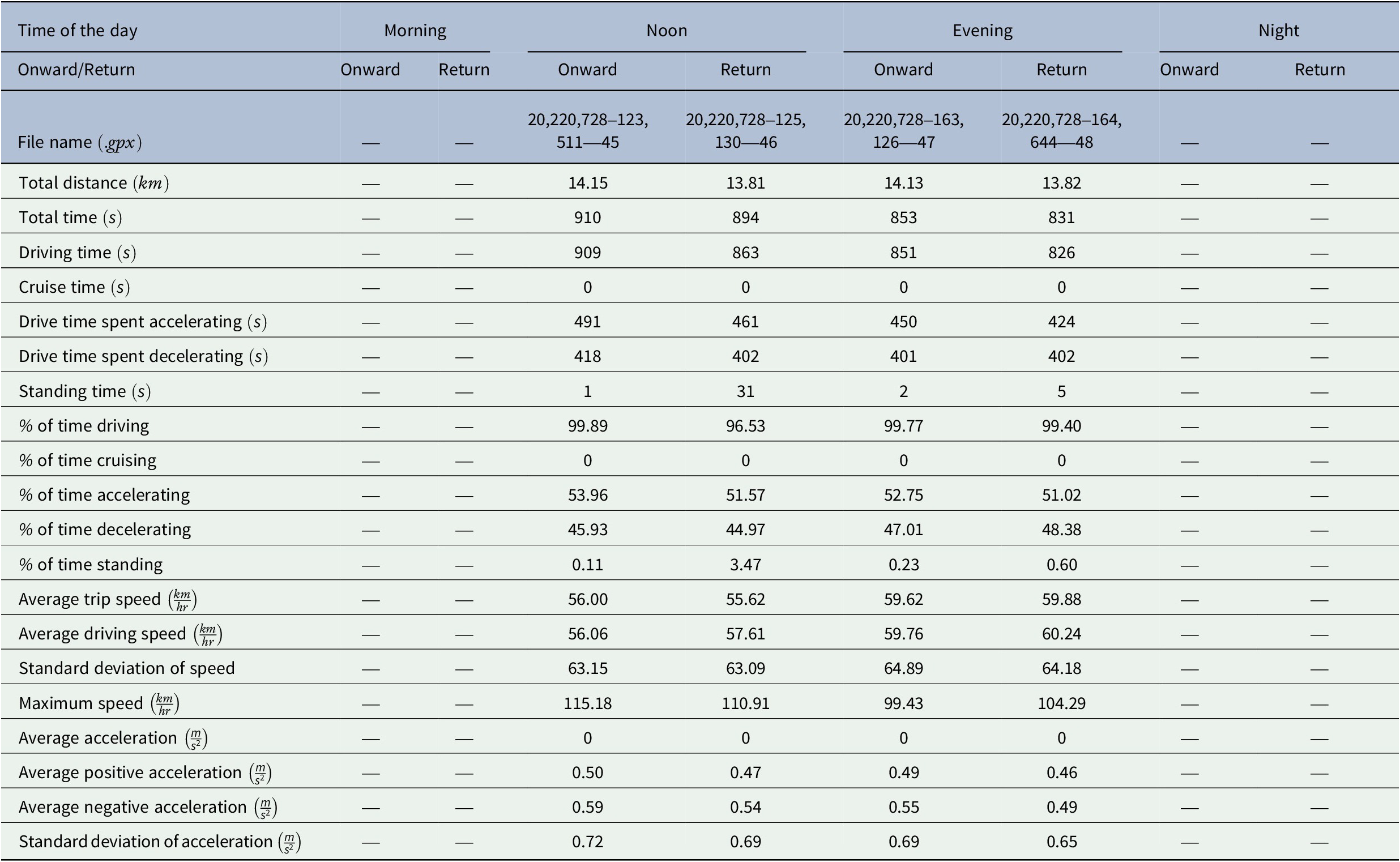
It should be noted that in these tables, the selected features for all driving data included the total time, total distance, idle time, cruise time, driving time, drive time spent for decelerating/accelerating, time for decelerating/accelerating, standing time, percentage of time driving, and time stopping. Other features included the average trip speed, average driving speed, standard deviation of speed, average or maximum speed, acceleration, and average negative/positive acceleration.
The results demonstrated that the time of day and the day of the week directly affect the time of driving and, consequently, other significant driving cycle characteristics in Semnan. Likewise, there are a lot of factors that can affect driving behavior, such as traffic congestion, pedestrian presence, the mood of the driver, and distraction factors during driving, which are not included in this article and could be tracked in further investigations.
In addition, to implement a sensitivity analysis, the Principal Component Analysis (PCA) method was used on the characteristics of raw data. Figure 1 shows the relative PCA coefficients of both vehicles via a double-legend bar chart.
Table 6. Characteristics of logged data on Wednesday, July 27, 2022, for the Prius
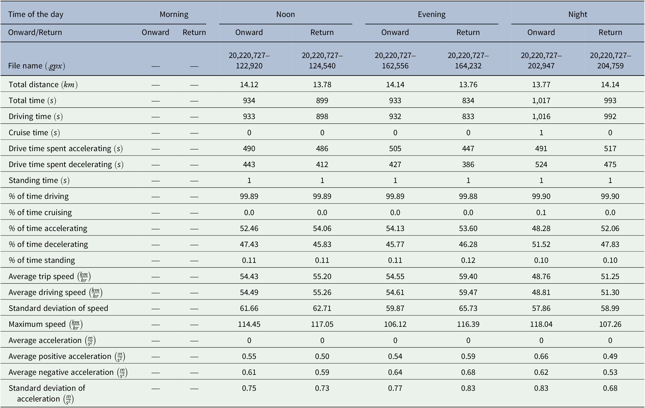
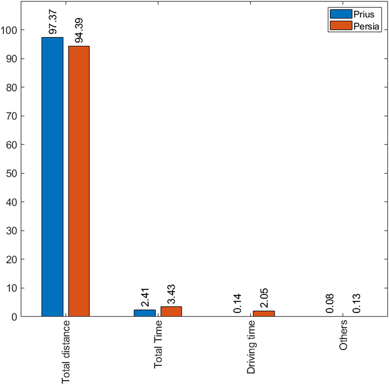
Figure 1. Relative PCA coefficients of both vehicles.
Table 7. Characteristics of logged data on Thursday, July 28, 2022, for the Prius
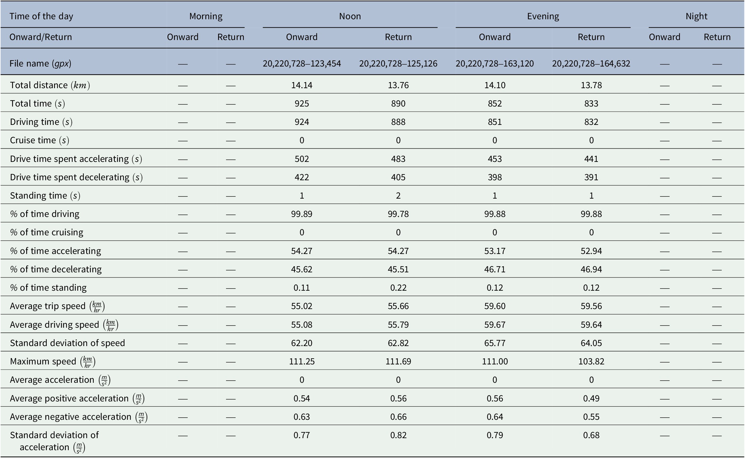
Table 8. Characteristics of logged data on Thursday, July 21, 2022, for the Persia
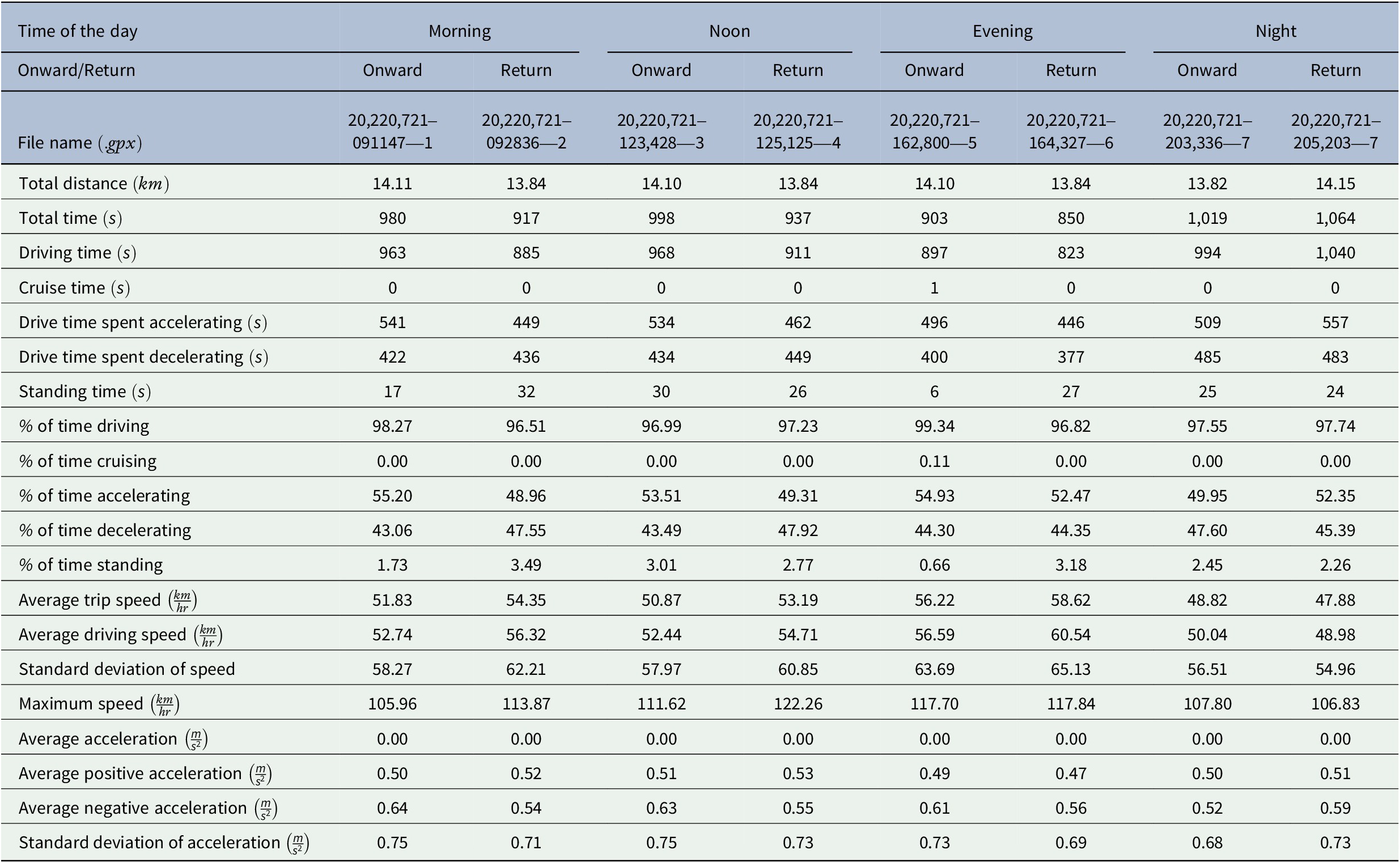
Table 9. Characteristics of logged data on Friday, July 22, 2022, for the Persia
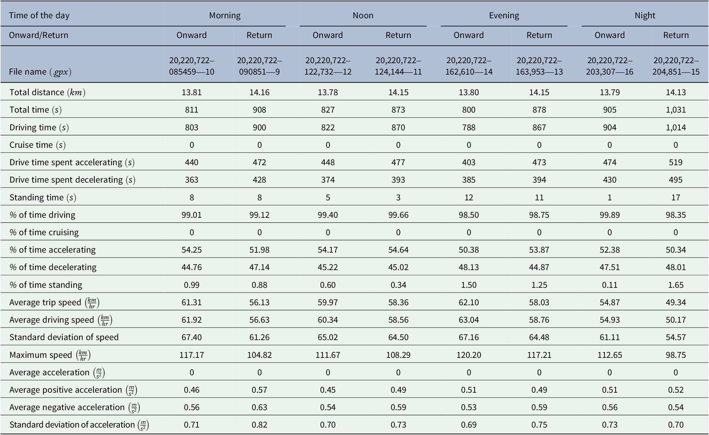
Table 10. Characteristics of logged data on Saturday, July 23, 2022, for the Persia
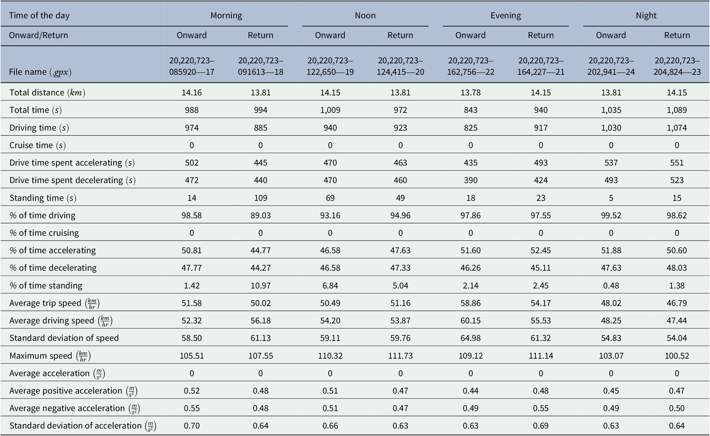
Table 11. Characteristics of logged data on Sunday, July 24, 2022, for the Persia
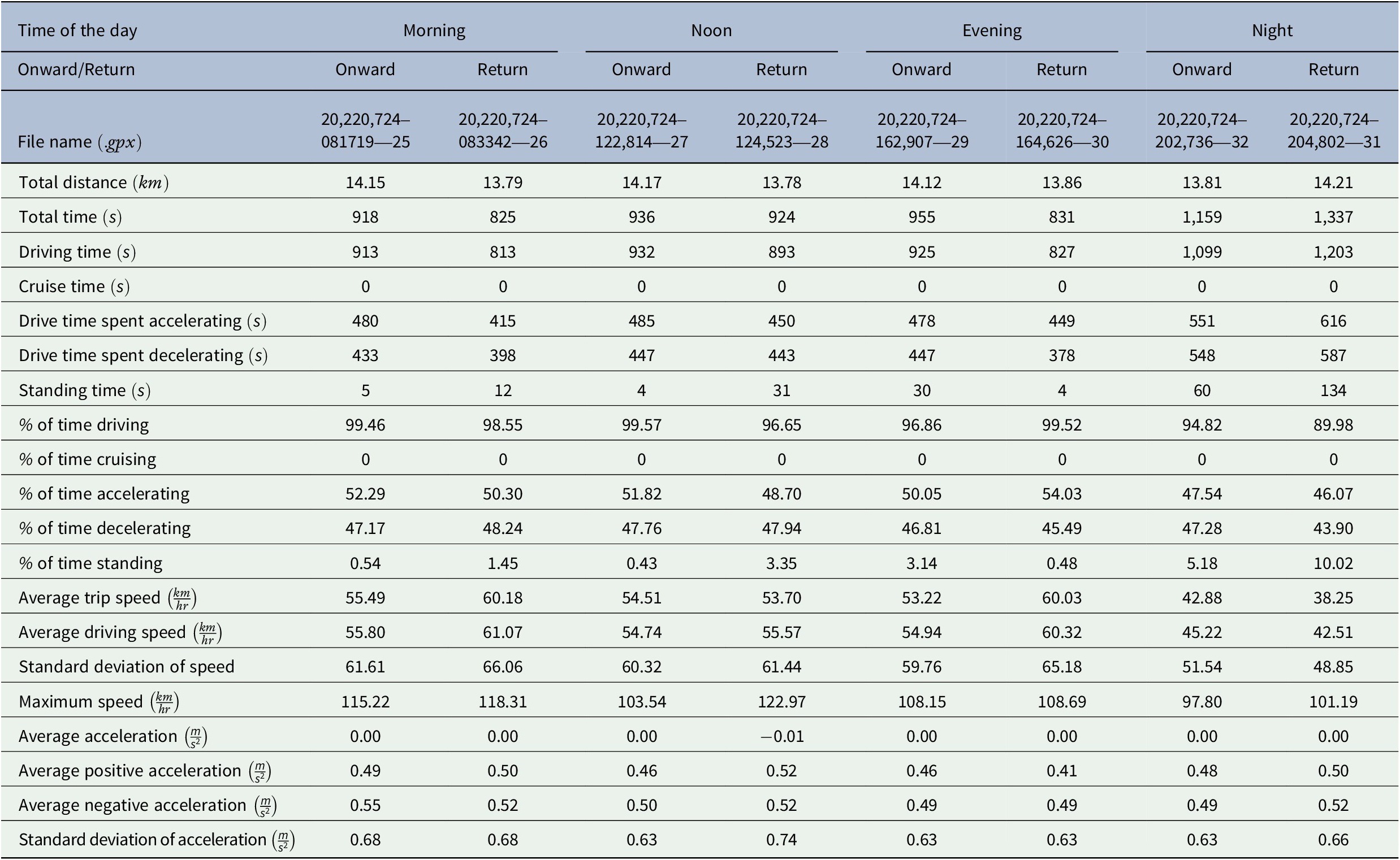
Table 12. Characteristics of logged data on Monday, July 25, 2022, for the Persia
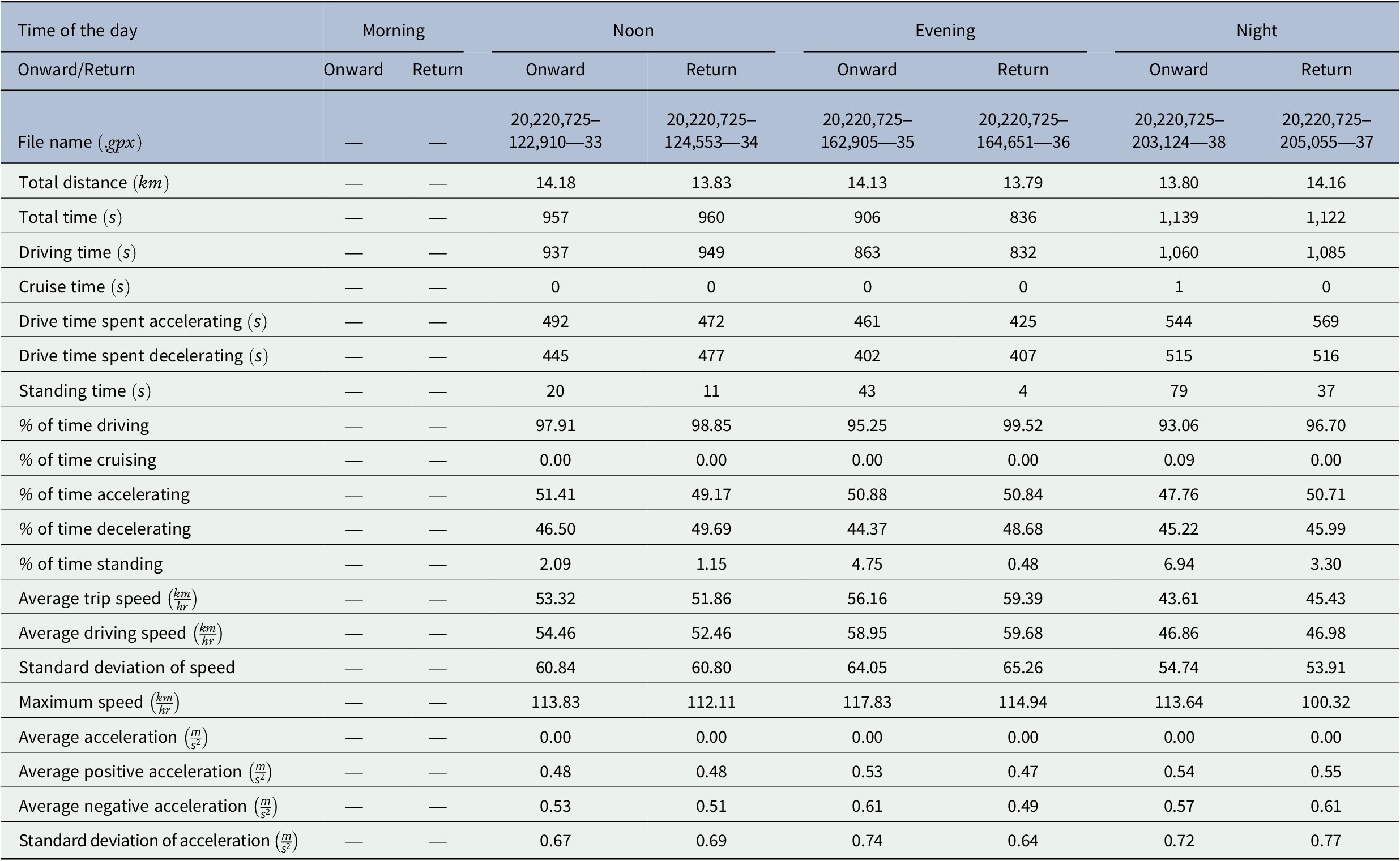
Table 13. Characteristics of logged data on Wednesday, July 27, 2022, for the Persia
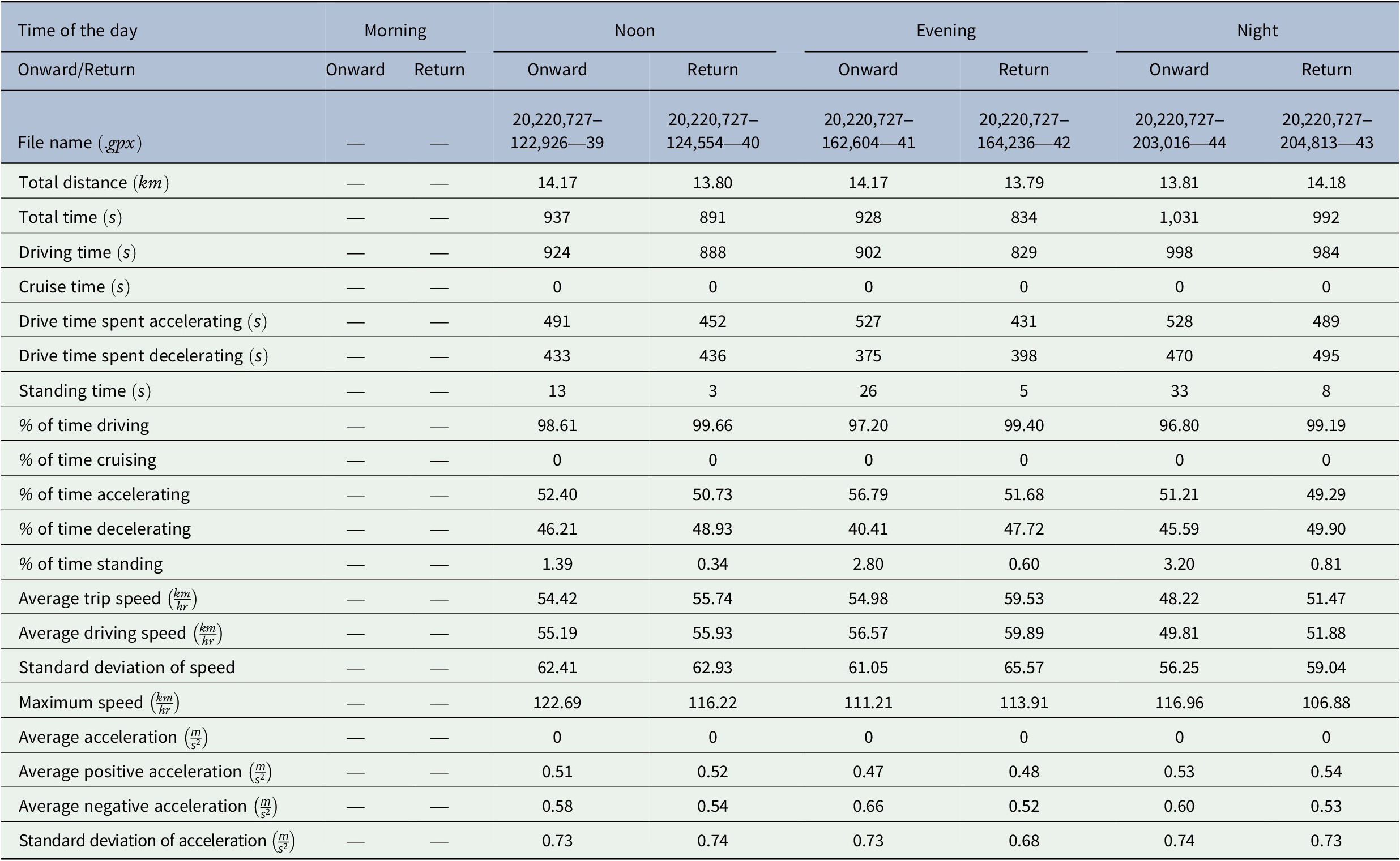
Table 14. Characteristics of logged data on Thursday, July 28, 2022, for the Persia
As expected, the relative PCA coefficient of “total distance” was 97.37%, and that of the “total time” was evaluated at almost 2.4% for all logged data. Figure 2 illustrates the scatter plot of these two driving cycle characteristics. The same procedure was used for Persia-related data but this time with the relative PCA coefficient of 94.4% for the “total distance” and around 3.5% for the “total time”. Figure 3 demonstrates the relation between them as well, for the Persia.
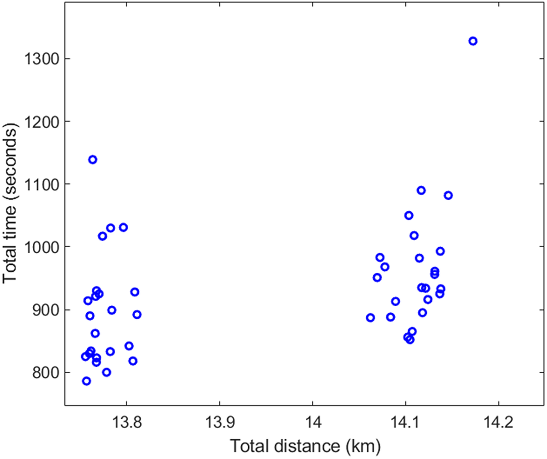
Figure 2. The scatter plot for two main parameters of data for the Prius.
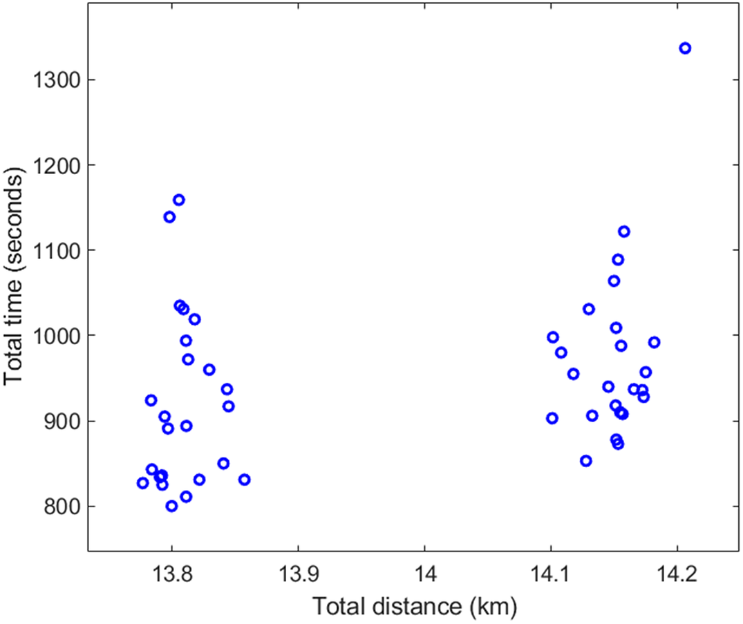
Figure 3. The scatter plot for two main parameters of data for the Persia.
Comparing the obtained results to the literature (Joubert & Grabe, Reference Joubert and Grabe2022; Miri et al., Reference Miri, Azadi and Pakdel2022; Onyekpe et al., Reference Onyekpe, Palade, Kanarachos and Szkolnik2021; Wawage & Deshpande, Reference Wawage and Deshpande2022), it could be claimed that there was an average error of 9% for the sensitivity of the most reliable PCA coefficients. Despite this, the order of the effective parameters was alike. In these references, many factors such as the driver behavior during driving (aggressive or defensive), the ground vehicle model (as mentioned in the literature (Joubert & Grabe, Reference Joubert and Grabe2022; Miri et al., Reference Miri, Azadi and Pakdel2022; Onyekpe et al., Reference Onyekpe, Palade, Kanarachos and Szkolnik2021; Wawage & Deshpande, Reference Wawage and Deshpande2022): Ford Fiesta Titanium, Pars Khodro Tiba, Isuzu FTR850, and Ford Figo 1.2), the driver age, the environmental scenarios, the road states, the selected route, the GPS update rate, the country, and the data acquisition methods (a diverse model of smartphones) differed from this work.
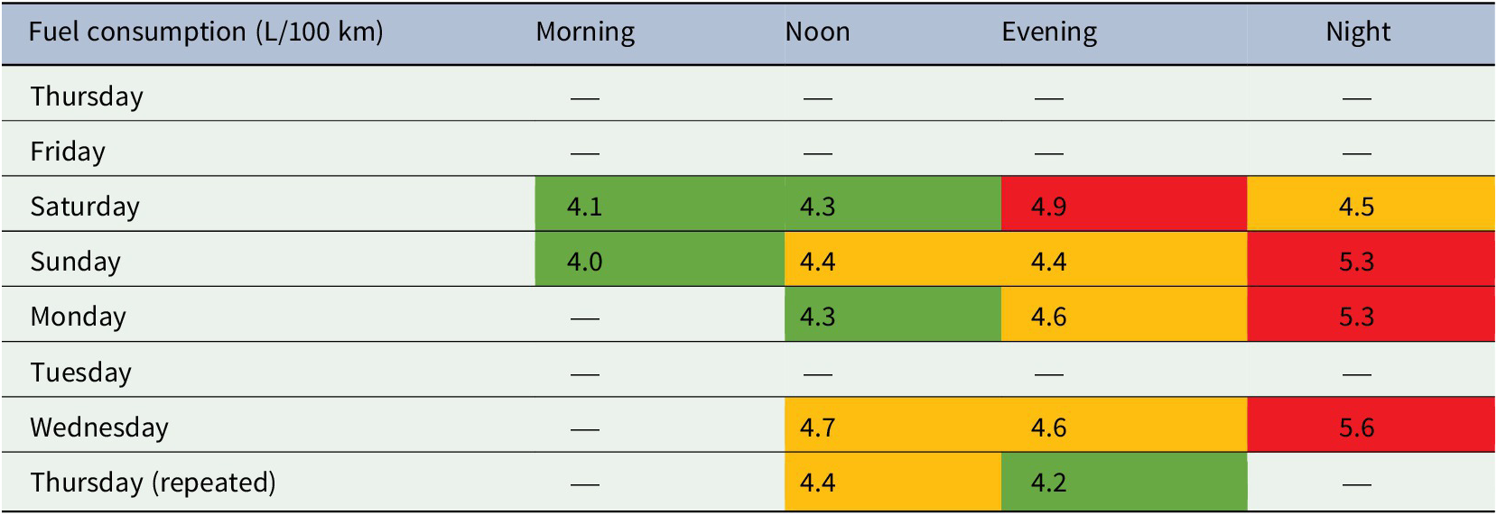
For the Prius, based on data obtained by the Electronic Control Unit (ECU), the fuel consumption was measured and is reported in Tables 15 and 16. Higher values are denoted in red and lower values are denoted in green. From these data, the fuel consumption is found to be between 3.7 and 6.1 L/100 km. As expected, the fuel consumption was highest for the onward drive route in the evening, when the traffic condition was at its worst. In the return drive route, the highest fuel consumption was found to be at night. Based on Table 16, the fuel consumption is observed to be between 4.0 and 5.6 L/100 km. The change in the driving behavior in the onward and return drive routes was due to the road slope.
Table 15. The fuel consumption for the Prius in the onward route based on ECU data
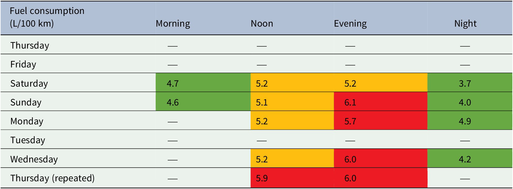
Table 16. The fuel consumption for the Prius in the return route based on ECU data
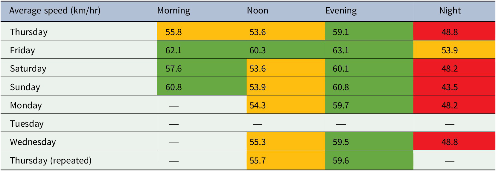
Furthermore, the average speed of the car is also depicted in Tables 17 and 18, based on the ECU data. Here, the implications of the colors green and red are reversed, with lower values being denoted with red and vice versa. The average speed was between 38.4 and 59.7 km/hr on the onward route and 43.5 and 63.1 km/hr on the return route. In both routes, the average speed of the Prius was lower at night as compared to the other times when data acquisition happened. In addition, speed was found to be higher in the evening. On Fridays, the average speed was found to be higher than that of the other days, since this day of the week is a holiday in Iran and consequently the traffic condition is lighter.
Table 17. The average speed of the Prius in the onward route based on ECU data
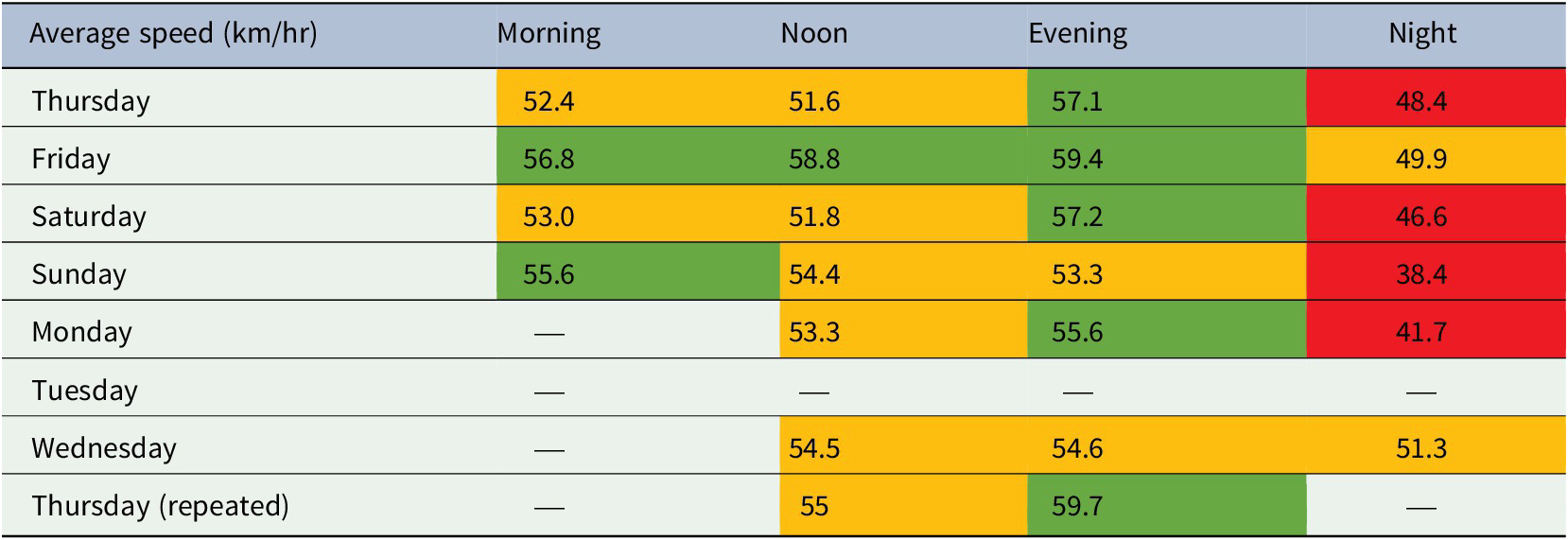
Table 18. The average speed of the Prius in the return route based on ECU data
Finally, to monitor and control traffic conditions that affect driving cycles, new technologies will need to be developed. As an example, Khosravi et al. (Reference Khosravi, Rezaee, Moghimi, Wan and Menon2023) presented a method to predict crowd emotion to understand more about human–vehicle interaction, using fuzzy logic ranking and modified transfer learning techniques. In this study, they utilized unmanned aerial vehicles with video surveillance capabilities to improve citywide traffic flow.
To discuss more the relationship between this data article and the literature (Khosravi et al., Reference Khosravi, Rezaee, Moghimi, Wan and Menon2023), it should be noted that the current study collected raw driving data from passenger cars in Semnan to gain a better understanding of traffic conditions and inform the improvement of urban transportation systems. This research contributes to the broader goal of creating more efficient and safe smart cities through the use of modern technology, which is a common goal also shared by other studies, such as the aforementioned research by Khosravi et al. (Reference Khosravi, Rezaee, Moghimi, Wan and Menon 2023). Thus, while this dataset focuses on driving data collection and analysis, it aligns with other research on modern technology to improve traffic flow and safety in smart cities. The combination of these approaches can lead to more efficient and safe urban environments, where transportation systems and public safety are improved through advanced technology and innovative methods.
Experimental design, materials, and methods
In this study, the impact of traffic conditions on driving data is presented for the city of Semnan in Iran. The map of this city and the road conditions are presented in Figure 4a. In this image, different roads with various speed limits are also illustrated, such as expressways (110 km/hr), main roads (80 km/hr), secondary roads (60 km/hr), and branch roads (40 km/hr).
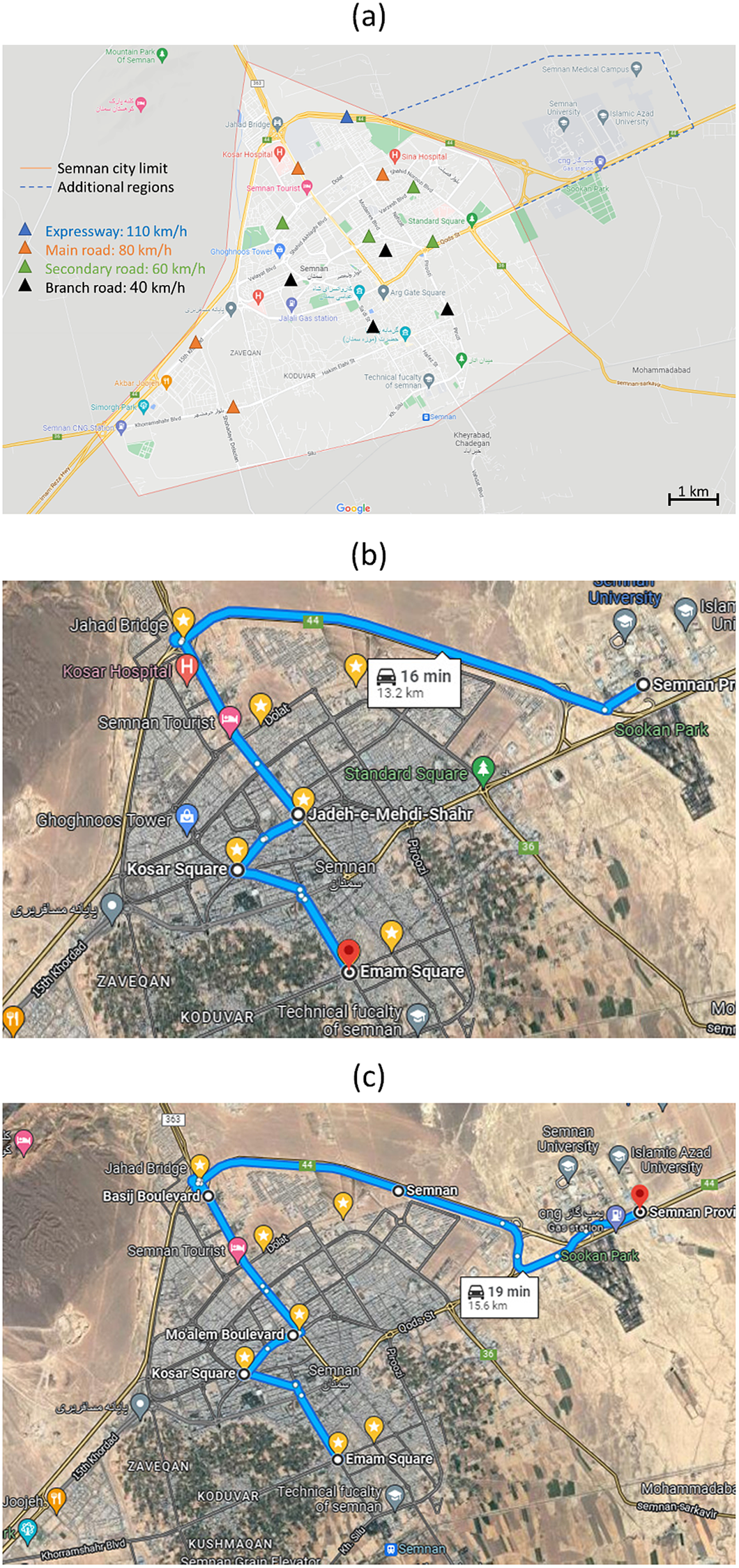
Figure 4. (a) A map of Semnan and the road conditions, with the route of data acquisition: (b) onward and (c) return.
In order to acquire driving data, two passenger cars or vehicles were used. One was a hybrid car combining an internal combustion engine with an electric module (the Toyota Prius), and another one had only an internal combustion engine (the Peugeot Pars, also known as the IKCO [IranKhodro Company] Persia in Iran, too). GPS sensors have been used for logging coordination data such as longitude, latitude, elevation, speed, and local time. For the route, the start point of the data logging was at Azad University, and the destination was Imam Market, both within the city. After reaching the goal, the driver took a brief break and returned the cars to the start point using the same roads. The route of data acquisition is depicted in Figure 4a,b, including 13.2 km of the onward journey and 15.6 km of the return journey.
It should be noted that the drivers for the Prius and Persia were men aged 33 and 25 years old, with 18 and 5 years of driving experience, respectively. Moreover, in the selected route, the Prius was followed by the Persia.
Based on this procedure, for about 670 km and 13 hours, driving data were acquired for 7 days. The above procedure was repeated every day for one week (except Tuesday, and twice on Thursday) and for four different times of the day (morning, noon, evening, and night). Details of data acquisition can be found in Table 19 for July 21–28, 2022 (from 07:00 to 22:00). In this table, light, moderate, and heavy traffic has been denoted by green, orange, and red colors, respectively; these data were obtained from Google Maps.
Table 19. The time of data acquisition in Semnan
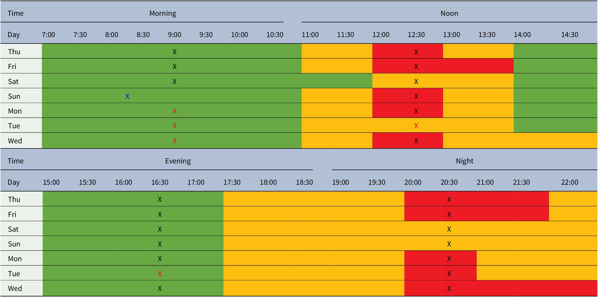
Note. X shows the time of data acquisition. A red-X means no data, while a blue-X means data at different times, due to limitations.
The traffic condition in Semnan could be compared to Mashhad, also a city in Iran, as presented in a study by Pouresmaeili et al. (Reference Pouresmaeili, Aghayan and Taghizadeh2018). They found that by the hourly measurements of air pollutant stations in Mashhad, the peak hour in the morning was found to be between 7:00 and 09:00, and in the afternoon it was between 16:00 and 18:00. However, these peaks were found to be between 12:00 and 12:30 in the morning and between 20:00 and 21:30 in the evening in Semnan city. It means that the configuration of the city has an impact on traffic conditions, even when both cities are located in one country (Iran).
In other words, the driving cycle consequently needs to be developed for each city, separately. As a confirmation, Kamble et al. (Reference Kamble, Mathew and Sharma2009) illustrated that the traffic condition in Pune (India) had large fluctuations due to heterogeneity and congestion, leading to higher variations in the vehicle speed, deceleration, and acceleration values.
The initial data can be found in the Mendeley Data (Azadi & Shahsavand, Reference Azadi and Shahsavand2023). These data include the speed versus the time, plus the GPS data (, and altitude).
Notably, each piece of data included the following: a “TXT” file, a piece of general information about the GPS data; a “GPX” file, a GPS exchange format, which is an XML file that is designed for the GPS data in the software applications; and a “KML” file, which is used to demonstrate the geographic data in an Earth browser).
Because of the low GPS accuracy of the utilized device for speed measurement, the car speed for each instant could be calculated using discrete derivatives of the car position. For this problem, the raw GPS data were imported to MATLAB using the “gpxread” command, as follows,
P = gpxread(‘file.gpx’);
where “file.gpx” refers to the file name of the raw data in the GPX file format. After the execution of the above line of code, the variable P would be a geo-point vector with feature properties.
The number of the collected points would be,
N = length(P.latitude);
Although this number could be found within the “TXT” format file, the GPX format was used for convenience. It could be possible to get the number of collected points using other properties instead of latitude. The “geopoint” also contains the recorded time of the GPS, though the format differs and should be converted to be recognized as a “datetime” class of MATLAB,
timeStr = strrep(P.Time,’Z’,’‘);
timeStr = strrep(timeStr,’T’,’ ‘);
t = datetime(timeStr);
The letters ‘Z’ and ‘T’ have to be removed in order to avoid getting errors. Finally, “datetime” function will convert the “cell” array to the “datetime” class. In the next step, the calculation of the distance between the collected points is required. Fortunately, MATLAB has a function for this problem as well,
e = wgs84Ellipsoid;
lat = P.latitude;
lon = P.longitude;
d = distance(lat(1:end-1), lon(1:end-1), lat(2:end), lon(2:end), e);
where “wgs84Ellipsoid” is the Reference ellipsoid for World Geodetic System 1984, and the “distance” function calculates the distance between the points on a sphere or an ellipsoid. By knowing the distance between the points, the velocity and the acceleration between every two points could be calculated; but first, the format of the date should be changed to seconds. Function “datenum” changes the “datetime” class to “double” (days number).
day2seconds = 24*3600;
dt = day2seconds*datenum(diff(t));
v = d./dt * 3.6;
v = [v 0];
a = diff(v/3.6)./dt;
a = [a 0];
where d, dt, v, and a are the distance, elapsed time, mean velocity, and mean acceleration between two data points, respectively. By knowing these values at each instance, the generation of the drive cycle can begin. The following equations have been derived from the literature (Onyekpe et al., Reference Onyekpe, Palade, Kanarachos and Szkolnik2021), with which the characteristics of the data can be demonstrated. The following definitions of the parameters are applied to n data rows of time in seconds, and i is the selected element of time, with $ 1\le i\le n $
and for velocities
$ 1\le i\le n $
and for velocities $ 1\le i<n $
.
$ 1\le i<n $
.
The total time, the total stop time, and the total distance of the data could be calculated as
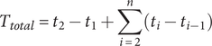 $$ {T}_{total}={t}_2-{t}_1+\sum \limits_{i=2}^n\left({t}_i-{t}_{i-1}\right) $$
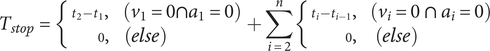 $$ {T}_{stop}=\left\{\begin{array}{c}\hskip-1em {t}_2-{t}_1,\left({v}_1=0\cap {a}_1=0\right)\\ {}\hskip1.2em 0,\hskip-6em (else)\end{array}\right.+\sum \limits_{i=2}^n\left\{\begin{array}{c}\hskip-1em {t}_i-{t}_{i-1},\left({v}_i=0\hskip0.35em \cap \hskip0.35em {a}_i=0\right)\\ {}\hskip1.8em 0,\hskip-5.6em (else)\end{array}\right. $$
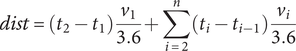 $$ dist=\left({t}_2-{t}_1\right)\frac{v_1}{3.6}+\sum \limits_{i=2}^n\left({t}_i-{t}_{i-1}\right)\frac{v_i}{3.6} $$
where $ {t}_i $
,
$ {t}_i $
, $ {v}_i $
, and
$ {v}_i $
, and $ {a}_i $
are the i-th elements of the local GPS time, vehicle velocity, and vehicle acceleration, respectively, and n is the number of data points collected. Having Equations (1) and (2), the “driving time” could be evaluated by Equation (4). Furthermore, the equations of “driving time spent accelerating” and “decelerating” are Equations (5) and (6), respectively.
$ {a}_i $
are the i-th elements of the local GPS time, vehicle velocity, and vehicle acceleration, respectively, and n is the number of data points collected. Having Equations (1) and (2), the “driving time” could be evaluated by Equation (4). Furthermore, the equations of “driving time spent accelerating” and “decelerating” are Equations (5) and (6), respectively.
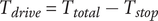 $$ {T}_{drive}={T}_{total}-{T}_{stop} $$
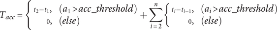 $$ {T}_{acc}=\left\{\begin{array}{c}\hskip-1em {t}_2-{t}_1,\left({a}_1> acc\_ threshold\right)\\ {}\hskip1.2em 0,\hskip-9.6em (else)\end{array}+\sum \limits_{i=2}^n\left\{\begin{array}{c}\hskip-1em {t}_i-{t}_{i-1},\left({a}_i> acc\_ threshold\right)\\ {}\hskip1.8em 0,\hskip-9.3em (else)\end{array}\right.\right. $$
 $$ {T}_{dec}=\left\{\begin{array}{c}\hskip-1em {t}_2-{t}_1,\left({a}_1<- acc\_ threshold\right)\\ {}\hskip1.2em 0,\hskip-11.4em (else)\end{array}+\sum \limits_{i=2}^n\left\{\hskip-1em ,\begin{array}{c}{t}_i-{t}_{i-1},\left({a}_i<- acc\_ threshold\right)\\ {}\hskip-2.6em 0,\hskip-11em (else)\end{array}\right.\right. $$
in which, the “acc_threshold” is one of the drive cycle parameters and should be determined considering the accumulation error of the sensors. This absolute value of the parameter defines if there is any acceleration or deceleration. According to Equations (4) and (5), the cruise time of the vehicle could be calculated as follows,
 $$ {T}_{cruise}={T}_{drive}-{T}_{acc}-{T}_{dec} $$
In addition, the percentage of $ {T}_{drive} $
,
$ {T}_{drive} $
, $ {T}_{cruise} $
,
$ {T}_{cruise} $
, $ {T}_{acc} $
,
$ {T}_{acc} $
, $ {T}_{dec} $
, and
$ {T}_{dec} $
, and $ {T}_{stop} $
, according to
$ {T}_{stop} $
, according to $ {T}_{total} $
, are represented in Equations (8) to (12).
$ {T}_{total} $
, are represented in Equations (8) to (12).
 $$ \% drive=\frac{T_{drive}}{T_{total}} $$
 $$ \% cruise=\frac{T_{cruise}}{T_{total}} $$
 $$ \% acc=\frac{T_{acc}}{T_{total}} $$
 $$ \% dec=\frac{T_{dec}}{T_{total}} $$
 $$ \% stop=\frac{T_{stop}}{T_{total}} $$
Equations (13) and (14) are related to “average speed” for a trip and “average driving speed”, using Equations (1), (3), and (4). Note that the unit of the “dist” is meters and the unit of all times is stated in seconds, though the fraction will be in $ \frac{m}{s} $
. By multiplying 3.6, the unit changes to
$ \frac{m}{s} $
. By multiplying 3.6, the unit changes to $ \frac{km}{h} $
.
$ \frac{km}{h} $
.
 $$ {\overline{v}}_{trip}=3.6\frac{dist}{T_{total}} $$
 $$ {\overline{v}}_{drive}=3.6\frac{dist}{T_{drive}} $$
The equation of “standard deviation of speed” is stated in Equation (15)). Note that $ v\_ sd $
corresponds to
$ v\_ sd $
corresponds to $ {\overline{v}}_{trip} $
and again the velocities are stated in
$ {\overline{v}}_{trip} $
and again the velocities are stated in $ \frac{km}{hr} $
.
$ \frac{km}{hr} $
.
 $$ v\_ sd={\sigma}_v=\sqrt{\frac{1}{n-1}\sum \limits_{i=1}^n{v}_i^2} $$
 $$ {v}_{max}=\max (v) $$
The same formulations are available for the acceleration of the vehicle in the unit of $ \frac{m}{s} $
as follows,
$ \frac{m}{s} $
as follows,
 $$ a\_ av=\overline{a}=\frac{1}{T_{total}}\sum \limits_{i=1}^n{a}_i $$
 $$ a\_ pos\_ av={\overline{a}}_{pos}={\left(\sum \limits_{i=1}^n\left\{\begin{array}{c}\hskip-1em 1,\left({a}_i>0\right)\\ {}\hskip-1em 0,\hskip-1em (else)\end{array}\right.\right)}^{-1}\sum \limits_{i=1}^n\left\{\begin{array}{c}\hskip-1em {a}_i,\left({a}_i>0\right)\\ {}\hskip-1em 0,\hskip-1em (else)\end{array}\right. $$
 $$ a\_ neg\_ av={\overline{a}}_{neg}={\left(\sum \limits_{i=1}^n\left\{\begin{array}{c}\hskip-1em 1,\left({a}_i<0\right)\\ {}\hskip-1em 0,\hskip-1em (else)\end{array}\right.\right)}^{-1}\sum \limits_{i=1}^n\left\{\begin{array}{c}\hskip-1em {a}_i,\left({a}_i<0\right)\\ {}\hskip-1em 0,\hskip-1em (else)\end{array}\right. $$
 $$ a\_ sd={\sigma}_a=\sqrt{\frac{1}{n-1}\sum \limits_{i=1}^n{a}_i^2} $$
For sensitivity analysis in the previous part, the PCA of raw data was used. For more information about this technique, the references (Barlow et al., Reference Barlow, Latham, McCrae and Boulter2009; Jackson, Reference Jackson1988; Jolliffe, Reference Jolliffe2002; Joubert & Grabe, Reference Joubert and Grabe2022; Krzanowski, Reference Krzanowski1988; Miri et al., Reference Miri, Azadi and Pakdel2022; Roweis, Reference Roweis1998; Seber, Reference Seber1984; Wawage & Deshpande, Reference Wawage and Deshpande2022) are recommended. Fortunately, there is a MATLAB function called “pca” in which there are a lot of options to use this method. The following command shows its input and outputs:
[coeff, score, latent, tsquared, explained, mu] = pca(X).
In the outputs, “coeff” is a short term for the PCA coefficients, which are also known as loadings in matrix X. The function returns the PCA scores and variances in the score and latent, respectively. For each observation in X, the function returns the Hotelling’s T-squared statistic in the variable of “tsquared”. In addition, the percentage of the total variance that is explained by each PCA and the estimated mean data in X are returned in explained and “mu”, respectively. Further information about how to use other inputs and plenty of examples are available in the MATLAB “pca” function document.
Finally, as a brief issue on the importance and the value of these data, the following points could be mentioned,
-
• The proposed raw data could be used for further investigations on the final driving cycle, measuring the fuel consumption and emissions, etc., in Semnan or other similar cities.
-
• These driving data are useful for design engineers in the field of city management or in the transportation or manufacturing vehicles.
-
• The dataset could be further utilized in analyzing the real driving emission (RDE), which is now under the consideration of countries for environmental laws.
-
• Moreover, researchers could use these raw data for any of their analyses of traffic and vehicles, both in civil and mechanical engineering.
-
• Governments could be another beneficiary for designing and managing the city.
Conclusions
Raw driving data was acquired for two passenger cars in the city of Semnan in Iran. The impact of traffic conditions during morning, noon, evening, and night on this data were then considered.
-
• Two male drivers, ages 33 and 25 years old, drove the Toyota Prius and the Peugeot Pars (or the IKCO Persia) to acquire driving data for 670 km (13 hrs) over a week (July 21–28, 2022).
-
• Using the GPS application, the data on speeds were acquired for both vehicles, in addition to the fuel consumption and the average speed (for initial verification of the application data) data collected through the ECU in the Prius.
-
• Based on the initial sensitivity analysis, the features of raw driving data were checked, and it was found that the “total distance” was the most effective feature. The “total time” feature ranked second and was evaluated at almost 2.4% for all logged data.
This raw data could be used by engineers to develop a driving cycle in Semnan for any design of vehicles and their related components, or any evaluation of emissions and fuel consumptions, or, also, any considerations in the transportation system in the future.
Acknowledgments
This data article did not receive any specific fund or grant.
Open peer review
To view the open peer review materials for this article, please visit http://doi.org/10.1017/exp.2023.11.
Data availability statement
The raw data could be found at Azadi and Shahsavand (Reference Azadi and Shahsavand2023).
Author contribution
Formal analysis: A.M.; Investigation: A.M., M.A.; Resources: A.M., M.A.; Software: A.M.; Writing – original draft: A.M., M.A.; Conceptualization: M.A.; Data curation: M.A.; Funding acquisition: M.A.; Methodology: M.A.; Project administration: M.A.; Supervision: M.A.; Validation: M.A.; Visualization: M.A.; Writing – review & editing: M.A.
Authorship contribution
Conceptualization: M.A.; Data curation: M.A., A.S.; Formal analysis: A.M., A.S.; Funding acquisition: M.A., A.S.; Investigation: M.A., A.M., A.S.; Methodology: M.A., A.M.; Project administration: M.A.; Resources: M.A., A.S.; Software: A.M.; Supervision: M.A.; Validation: M.A.; Visualization: M.A., A.M., A.S.; Writing–original draft: A.M.; Writing–review & editing: M.A.
Competing interest
The authors declare that they have no known competing financial interests or personal relationships.


 Open access
Comments
The comments are attached