


Social media summary: Analysis of over 35,000 historical individuals reveals peaks and troughs of residential mobility in the life course
1. Introduction
Mobility is both an important and diverse form of human adaptation: from the spread of our species out of Africa, to the resource mapping of hunter–gatherer groups, through the relative immobility and high landscape investment of agricultural populations, to the renewed mobility of contemporary urban labour networks. Mobility allows humans to flexibly respond to their circumstances. Changes in mobility patterns are implicated in every major economic transition, from foraging to domestication to urban settlement and resettlement. The consequences of mobility for landscape alteration (Bird et al., Reference Bird, Bird, Codding and Taylor2016; Kelly et al., Reference Kelly, Poyer and Tucker2005) and cultural evolution (Boyd & Richerson, Reference Boyd and Richerson2009; Perreault & Brantingham, Reference Perreault and Brantingham2011; Soltis et al., Reference Soltis, Boyd and Richerson1995) are also significant. Therefore the contribution of mobility to human adaptation is not only a basic research question for human evolution. It is also of critical importance for understanding contemporary responses to environmental and social change, enabling better prediction and planning, especially in light of ongoing climate adaptation (Pisor & Jones, Reference Pisor and Jones2020).
In this study we present a quantitative life course perspective of individual mobility in a sedentary, urbanising, but nonetheless mobile population. We focus on describing residential mobility and how it patterns over the life course of thousands of individuals. The individual nature of the records allows us to describe variation in life course trajectories related to mobility, not just population or group averages. Our goal is to demonstrate that sedentary, even urban, populations are highly mobile and that their mobility is strategic, structured as it is over the life course of individuals. While we do not develop a full adaptive picture of mobility, we do support the importance of individual mobility in human adaptation and relate it to important questions in the study of human adaptation and cultural evolution.
Also, as we show, just to accurately describe mobility at the high resolution necessary for theory construction and testing is not trivial. Special care is needed to robustly estimate age-specific behaviour and individual variation, and then to produce valid projections to the target population. So in addition to providing a high-resolution description of individual mobility in a particular population, we also provide a detailed computational example of how these steps can be accomplished at scale with modern machine learning algorithms. Since all inferential work depends upon proper descriptive work, a scalable computational workflow is a contribution of its own.
Evolutionary approaches to both mobility and sedentarisation have tended to focus on the ecological drivers experienced by mobile peoples (Bettinger et al., Reference Bettinger, Garvey and Tushingham2015; Binford, Reference Binford1980; Kelly, Reference Kelly2013). Research in this literature explains mobility as a means of averaging over both spatial and temporal variation in resources. It is a way to manage risk and uncertainty (Cashdan, Reference Cashdan, Smith and Winterhalder1992), with hunter–gatherer mobility regimes forming a forager–collector spectrum (Kelly, Reference Kelly2013). The spectrum has recently been combined with more mechanistic views of hunter–gatherer mobility that explicitly link mobility decisions at the group and individual level to calories required (Hamilton et al., Reference Hamilton, Lobo, Rupley, Youn and West2016; Venkataraman et al., Reference Venkataraman, Kraft, Dominy and Endicott2017).
A similar framework has been usefully applied to understanding sedentarisation. Kelly argues that reduced mobility is a feature of ‘local abundance in regional scarcity’ (Kelly, Reference Kelly2013). Populations can reduce mobility if abundant resources are available, but those resources must be clustered in space, and time. Historically, hunter–gatherers located in rich environments tended to be more sedentary (e.g. Jomon: Crema, Reference Crema2013). These groups settled near marine resources, which follow the ‘abundance in scarcity’ profile: they are high value and clustered in time and space. Agricultural groups on the other hand create abundance locally. Through domestication, they cluster resources in a much smaller area, shifting to a sedentary life (O'Brien & Laland, Reference O'Brien and Laland2012).
The broad picture emerging from this work is that human groups have gradually reduced mobility as economies have increasingly focused on immobile resources and urban infrastructure. Yet we know this is wrong. Urban populations, contemporary and historical, can be highly mobile, much more mobile than traditional agricultural communities. This point was elucidated already by Zelinsky (Reference Zelinsky1971), who suggested that demographic transitions are accompanied by mobility transitions, which see the increase of mobility with ‘modernisation’.
A longstanding issue in both human behavioural ecology and cultural evolution is the integration of global, market-oriented livelihoods into theoretical frameworks that have been developed and tested mostly in ‘small-scale’ societies (Nettle et al., Reference Nettle, Gibson, Lawson and Sear2013). In the past decades research in Human Behavioral Ecology has worked to expand out of ‘small-scale’ populations. However, not all theory has been successfully translated. As Nettle et al. (Reference Nettle, Gibson, Lawson and Sear2013) point out, Human Behavioral Ecology has much to say on topics relating to reproduction, and much less on spatial patterning and resource use. This difference can also be seen in how our understanding of mobility is carried over, with work on kin co-residence finding industrial counterparts, while work on mobility regimes remains biased towards small-scale populations.
A mature account of adaptation, spanning economies and time periods, must address mobility post-sedentarisation, because people in sedentary and urban societies are not immobile, and their mobility is not random but rather makes strategic use of urban environments (Clech et al., Reference Clech, Jones and Gibson2020; Gillespie, Reference Gillespie2017; Kok et al., Reference Kok, Mandemakers and Wals2005). So while it is clear that populations living in sedentary settlements will not map on to the resource landscape in the same way as foragers, this does not preclude them from using mobility adaptively. Evolutionary theory and its strong connections to life history, tradeoffs and cultural evolution has an important role in explaining constructed environments and their associated mobility regimes. In turn, the study of human mobility in ‘sedentary’ systems may provide general insights for the study of human adaptation.
Describing mobility in extensive systems of permanent settlement and in the urban environments that characterise the Anthropocene (Lobo et al., Reference Lobo, Alberti, Allen-Dumas, Arcaute, Barthelemy, Bojorquez Tapia and Youn2020) requires extending evolutionary theory to account for the full diversity of human mobility strategies. Accomplishing this is necessarily complex. There are new issues to consider when attempting to characterise mobility in a ‘large-scale’ society, but the vast and high-resolution data potentially available from urban and urbanising contexts may make it possible to address both new and old questions with greater rigour. Crucially, total mobility for many historical hunter–gatherer groups is nearly always described with one number, or a range, depicting the number of group moves per year (Hamilton et al., Reference Hamilton, Lobo, Rupley, Youn and West2016; Kelly, Reference Kelly2013). That is, we know relatively little about the actual individual distributions of mobility in these societies, frustrating our ability to evaluate how mobility regimes are built up from individual trade-offs. While total annual residential moves are an important behavioural measure, it would be beneficial to understand the variation in terms of these moves as experienced by individuals within these societies. Particularly if we want to compare mobile and ‘sedentary’ groups, we need an understanding of what the distribution of mobility looks like over the population. For hunter–gatherer groups that exclusively move as a group, variation is expected to be low. However, a group average is already misleading for groups that engage in high amounts of logistic mobility. In large-scale permanent settlement systems, the diversity of lifeways afforded through varying economic pathways leads us to expect a fair amount of individual variation that is currently not described and surely under-theorised.
Although there are logistic difficulties related to collecting individual data on mobility, when mobility has been utilised to address hypotheses related to human reproduction and sex differences, individual data has been crucial (Cashdan et al., Reference Cashdan, Kramer, Davis, Padilla and Greaves2016). A review of the literature conducted in 2016 indicates that men range farther than women in a diversity of cultures and environments, and that this difference is consistent through much of the life course (Cashdan et al., Reference Cashdan, Kramer, Davis, Padilla and Greaves2016). Recent work on mobile foragers, using precision tracking equipment, provides high-resolution data on individuals and variation among them. The results support the trend: men travel further and have larger ranges (Wood et al., Reference Wood, Harris, Raichlen, Pontzer, Sayre, Sancillo and Jones2021).
The pattern also holds outside of subsistence societies. Ecuyer-Dab and Robert (Reference Ecuyer-Dab and Robert2004) find that men's personal travel ranges were 1.8 times larger than those of women in an industrial context. Analysis of mobile phone data shows that women visit fewer unique locations and travel shorter distances than men in Santiago, Chile (Gauvin et al., Reference Gauvin, Tizzoni, Piaggesi, Young, Adler, Verhulst and Cattuto2020). Studies across Auckland, Dublin, Hanoi, Helsinki, Jakarta, Kuala Lumpur, Lisbon and Manila also conclude that women tend to travel shorter distances (Ng & Acker, Reference Ng and Acker2018). If we consider residential mobility, the picture is more complicated, however, not least because residential mobility is often engaged in by households, not individuals. A study of young adult home leavers in East Germany shows greater mobility for females in terms of distance travelled, as more females moved to West Germany than males (Geissler et al., Reference Geissler, Leopold and Sebastian2012). Likewise, a study utilising individual panel data in Senegal suggests that women are more likely than men to migrate, but they tend to travel shorter distances (Chort et al., Reference Chort, de Vreyer and Zuber2020).
The picture emerging from this literature is that women tend to travel shorter distances, but move residence more often. This higher residential mobility for women was already documented in Ravenstein's ‘The Laws of Migration’, a keystone work in mobility studies based on historical census data (Ravenstein, Reference Ravenstein1889). However, reconsideration of this research has suggested that the female bias in internal migration is a feature of males leaving the population at a higher rate (through emigration or death), emphasising the need for the careful consideration of demographics when forming conclusions about mobility regimes (Alexander & Steidl, Reference Alexander and Steidl2012).
Analysing mobility over individual factors other than sex is uncommon in the evolutionary literature. Age in particular offers a way to begin to unpack the life history of mobility, thus uncovering the changing trade-offs experienced by individuals as they move through time. Relating sex differences to the life course, sex differences are already present in adolescence; for example a study with the Tsimane found that males had larger ranges than females during adolescence (Miner et al., Reference Miner, Gurven, Kaplan and Gaulin2014). While work on children's mobility is more sparse, research suggests more equal mobility behaviour (Davis & Cashdan, Reference Davis and Cashdan2019), but the small sample size and methodological treatment in this study warrants cautious conclusions. Considering the opposite end of the lifespan, some research points to continued female mobility in older age. For example, Wood and Marlowe (Reference Wood and Marlowe2011) show that grandmothers tend to be in camps with their daughters until daughters have teenage daughters of their own. This allows grandmothers to go where their help most increases their inclusive fitness (Jones et al., Reference Jones, Hawkes, O'Connell, Hewlett and Lamb2005). This work could perhaps be an indication that females move residence more than men in older age. Recent work by Wood et al. (Reference Wood, Harris, Raichlen, Pontzer, Sayre, Sancillo and Jones2021) will prove most valuable in comparison with similarly high-resolution data on lifespan mobility in non-foraging populations, such as studies by Gillespie (Reference Gillespie2017) and Ghosh et al. (Reference Ghosh, Berg, Bhattacharya, Monsivais, Kertesz, Kaski and Rotkirch2018), which utilise a life course approach to show variation over age in contemporary American and Finnish populations.
We take inspiration from these studies, but the unique nature of our sample allows us to evaluate individual variation in life course mobility and directly estimate the age-based effect. The sample we use is the Historical Sample of the Netherlands (HSN), a relational database of a sample of the Dutch population born in the Netherlands between 1850 and 1920 (Mandemakers, Reference Mandemakers2017). The HSN is a valuable resource as it contains individual life courses constructed both from birth/death certificates and, crucially for our purposes, dynamic population registers that contain all of the addresses within the Netherlands at which a research person (RP) was registered. Each municipality was responsible for keeping their records up to date, and so individuals were obliged to inform their municipality of any changes to residence, thus making this a dynamic record of their migration histories. As such, it is possible to track RPs through their lifetime residential moves. Moreover, given the time span the HSN addresses, it is well-positioned to address changes to mobility brought about by industrialisation. Historical sources from early industrialisation hotspots provide a unique lens through which to interrogate changes that both market integration and industrialisation may bring (Mattison & Sear, Reference Mattison and Sear2016). Finally, the HSN is a very large database, containing information on over 37,000 research persons. This size allows for greater analytic power as well as the possibility of addressing informative subsets of the population. Given its historical depth and high resolution, the HSN thus represents a unique and valuable resource for addressing historical and transitional lifeways.
We use the HSN to address two core questions about the life course of individual mobility in a system of permanent settlements. These questions address our primary goal of demonstrating the high levels of structured mobility in an urbanising population of sedentary communities. The descriptions we provide do not test specific adaptive hypotheses, but they do justify in great detail the claims that sedentary populations can be highly mobile, that mobility is strongly related to human life history and therefore plausibly to basic evolutionary considerations, and that these facts can lead to the cultural evolution of the landscape and of mobility patterns.
The first question we consider is: how many times do individuals change residence in this sample? This is the coarsest perspective on the data, and allows us to establish how much mobility individuals in the sample engage in.
Second, we investigate how residential mobility is patterned over the life course. To address this question, we describe the pattern of residential mobility by age, both in conjunction and separate from the demographic composition of the sample. Characterising individual mobility in this way allows us to show how aggregate mobility arises from the combination of individual pathways with population-specific fertility and mortality patterns. We also establish whether there is change in the age-based pattern over the cohorts in the HSN.
We stratify each of these results by gender to relate clearly with the existing rich literature on sex differences in mobility.
2. Methods
2.1. Data
The HSN is a relational database containing individual life courses from the nineteenth- and twentieth-century Netherlands. Constructed around so-called research persons (RPs), the HSN follows RPs from the cradle to the grave, constructing life course trajectories with information about birth and death dates, occupation, religious affiliation and migration. Moreover, individuals related to RPs are also surveyed, providing information on family composition, children and household mobility. As such, the HSN constitutes a rare resource, combining high-resolution and longitudinal data on a large sample of a historical population.
Detailed information about the database can be found in Mandemakers (Reference Mandemakers2017). The database is constructed from information contained in birth, death and marriage certificates, as well as dynamic population registers in the later years. Standard civil registration of birth, deaths and marriages began in the Netherlands in 1812, while population registers were instituted in 1850. The state of these data in the Netherlands is of exceptionally high quality, as two copies of all certificates were kept. Moreover, dynamic population registers going this far back are rare (Mandemakers, Reference Mandemakers2017).
The HSN is curated by the International Institute of Social History, Amsterdam (https://iisg.amsterdam/en/hsn), which manages access. In this project we work with the HSN Data Set Life Courses Release 2010.01 which contains 37,137 life courses of RPs. For cohorts present in the database, the curators have taken a random sample of the historical population to select RPs (sample ratios for cohorts: 1812–1872, 0.0075%; 1873–1902, 0.005%; 1903–1922, 0.0025%). This random sampling is important as individuals were not selected based on mobility, our variable of interest.
2.2. Population and historical context
Starting in the later half of the nineteenth century, the territory of the Netherlands industrialised. High population growth and increasing wealth replaced the dip experienced at the end of the Dutch Golden Age (seventeenth and eighteenth centuries). Karel et al. (Reference Karel, Vanhaute and Paping2011) describe the transition in the nineteenth and twentieth centuries as that of the emergence of a ‘modernised’, family-based agriculture and transitional lifestyles whereby more engagement occurred between those in the rural and urban landscapes. The authors label the transition as a process of ‘deruralisation’ to reflect not the total urbanisation of the population, but rather a restructuring of what it meant to be rural, as agricultural lifeways became integrated with the market and finally homogenised into a form of twenty-first-century agriculture (Karel et al., Reference Karel, Vanhaute and Paping2011).
In the seventeenth century, the Dutch republic was arguably the richest country in the world. This economic peak was the result of the Dutch empires’ productive mercantile capitalism (Steckel & Floud, Reference Steckel and Floud1997). Owing to what is argued to be the hangover from this success (high wages and a commitment to trade over industry), the Netherlands industrialised comparatively late (Mokyr, Reference Mokyr1974). With industrialisation, the Dutch economy picked up again by 1850, and 1850–1920 represented a period of both economic and population growth (Steckel & Floud, Reference Steckel and Floud1997). In fact, between 1800 and 2000, the population of the Netherlands multiplied 8 fold, thus establishing the highest population growth rate in Europe (Karel et al., Reference Karel, Vanhaute and Paping2011). This population growth was the result of falling death rates, rising life expectancy and high birth rates (Karel et al., Reference Karel, Vanhaute and Paping2011).
We use a national sample in this study. So it is important to note that despite its small size the Netherlands is relatively diverse, both ecologically and socially. Steckel and Floud (Reference Steckel and Floud1997) make the case for the ‘three Netherlands’, dividing the area along the lines of urban, non-urban market-oriented agriculture and subsistence-oriented agriculture. The urban area, mostly represented by North and South Holland and Zeeland, constitutes the core of the maritime empire of the Dutch republic. Many rural environments in these areas were occupied by specialist farmers that supplied to the market (mainly dairy farming/animal husbandry). This was also true of the North (Groningen, Friesland). The inland portions of the country on the other hand had poorer soils and were generally less connected to the national economy, with the exception of peat exports (Steckel & Floud, Reference Steckel and Floud1997; see Figure 1).

Figure 1. Province map of the Netherlands in circa 1920, greyscale for province boundary distinction, reproduced from Ekamper et al. (Reference Ekamper, van Poppel, Mandemakers, Merchant, Deane, Gutmann and Sylvester2011).
These differences in ecology and resulting subsistence systems had effects on the social organisation, economy and mobility of the local population. Dairy farming tended to produce surplus children, as land was already scarce, and farm work neither divisible nor intensive enough to benefit from large family sizes, thus this surplus population generally found its way to the cities. In contrast, the subsistence agriculture of the inner regions benefited from large family sizes, and children could thus find work locally (Adams et al., Reference Adams, Kasakoff and Kok2002). Speaking to the urban–rural divide, given the early development of mercantile capitalism in the Dutch republic, Dutch cities were subject to fluctuations in international markets, while rural areas, particularly those more inland geared towards self-sufficiency, experienced these fluctuations less (Steckel & Floud, Reference Steckel and Floud1997). From ca. 1840, the growth and densification of railway transport in the Netherlands interacted with the re-urbanisation of the population, such that areas of railway network growth were positively correlated with municipal population growth (Koopmans et al., Reference Koopmans, Rietveld and Huijg2012). Marriage rates were higher in urban areas. Deruralisaiton made it possible to marry and start a family younger, perhaps due to increased income sources, such that the mean age at marriage in the Netherlands dropped from above 27 in 1860 to just under 23 in 1970 (Karel et al., Reference Karel, Vanhaute and Paping2011).
Neolocality was the main post-marital residence form throughout the Netherlands in the study period, with only 10% of families living in extended households. Until the end of the nineteenth century, a system of live-in house help was the norm, particularly for agricultural households (Karel et al., Reference Karel, Vanhaute and Paping2011). For small-hold farmers, children would stay home until the age of about 12–14, and then begin work on someone else's farm or enter into domestic service, until marriage. It was only after marriage that individuals were able to start their own holding (Karel et al., Reference Karel, Vanhaute and Paping2011).
2.3. Data management and analysis
Statistical models were fit with the Stan engine, specifically CmdStan version 2.27.0 (Stan Development Team, 2021). All summaries and data management were conducted in RStudio version 1.4.1106, using R version 4.0.4 (R Core Team, 2014). All code associated with this manuscript can be found in the following github repository: https://github.com/Naty-fedorova/Dutch-historical-mobility.
Working with a secondary dataset involves a number of data checks and transformations. The resulting tables used in the analysis are summarised in Table 1. Firstly, we create working files from the original relational tables, where we translate column names and remove columns that we do not require for the analysis. Subsequently, we construct subsets of the data for particular components of the analysis, as well as carrying out logical checks on the data (e.g. does death year follow birth year?). We create a new dataframe of cleaned data, combining birth and death information with registration events, and constructing the number of moves and age at move variables. In this dataframe, individuals are not necessarily tracked from birth to death, but can be tracked for only a snapshot of their lives. The cleaned data is transformed whereby non-move events are given their own rows and subsequently used in the Poisson regression, as the analysis dataframe. We also create a subset from the cleaned data which includes only individuals for whom we have both a birth year and a death year, and can thus reconstruct the entire life course and associated residential mobility; this is the life course dataframe and is used for visual analysis.
Table 1. Historical Sample of the Netherlands (HSN) subsets created and used in this study

RP, Research person.
2.4. Variables
Moves per year
Mobility is tracked in the HSN in a relational table containing information on addresses at which an RP was registered. As we are interested in mobility (i.e. residential moves), we remove the first registered address for an RP if this address occurs at birth to create a count of moves per RP. If the RP in question does not have an address at birth, we do not remove their first logged registration and assume that they have moved to their first logged address from somewhere.
The dynamic population registers from which the registration events originate were based around households, not individuals. We postulate that this is the reason why many registration events (43, 738) occur prior to RP birth, as registration events from the household of birth are transplanted to the RP. We deal with these registration events as follows: for RPs with a registration event at age 0, we remove all prior registration events. For a RP with no registration event logged at age 0, we coerce the closest (in years) registration event to occur at the birth year of the RP. If several registration events occur in this closest year, we coerce all of them to the birth year. Similarly, there are many registration events occurring after an RPs death year, or where absent, after the end of observation for a given RP (11,882). We remove these data points as well.
Age
Age at move is constructed from the birth year information and the address start year information. In principle, the address start year should log when a RP (and associated household) registered at a particular location. Of course, in practice, individuals often register within varying time spans of arriving at an address. As such, we keep to a resolution of one year.
Gender
Gender is directly extracted from the HSN database, translated, and recoded to 1 = female, and 2 = male.
Research person ID
Each RP has a unique ID in the HSN database. We check these for uniqueness and construct our own for posterity.
2.5. Statistical analysis
In order to analyse how the number of residential moves per year changes with age, we fit an over-dispersed Poisson regression model to estimate the number of moves a RP has each year (yi) for the years they are observed:


where λ i represents an expectation for each case i in the data (an individual, with a specific gender, at a specific age, with a given number of moves), which is a function of a sample average μ, a unique offset estimated for each individual $\alpha _{{\rm person}\_{\rm i}{\rm d}_{\rm i}}$ , and an age-specific offset $\beta _{{\rm ag}{\rm e}_i, {\rm gende}{\rm r}_i}$
 , which is calculated for each gender (equation 2).
Given that we can have multiple and varying numbers of observations per RP, a varying effects model clustered on RP IDs allows us to estimate individual variation. The varying effects methodology allows us to account for filtering concerns brought about by systematic differences in mobility between individuals.
Age-specific responses $\beta _{{\rm ag}{\rm e}_i,{\rm gende}{\rm r}_i}$ are modelled with two Gaussian processes, one for each gender. The Gaussian process estimates continuous functions of age, so that no assumption is made about the shape of this function, only that it changes smoothly so that close ages are more similar in their response. Specifically, we assume that for gender g the covariance in response between any pair of ages l and m of different distances $K_{lm}$
 is determined by:

This function states that the covariance Klmg between any two ages l and m declines exponentially with the squared distance Dlm between them. The parameter ηg 2 represents the maximum covariance between any two ages. The parameter ρg 2 determines the rate of decline in covariance (see McElreath, Reference McElreath2020 for a textbook treatment). The Gaussian process approach allows us to account for censoring concerns given the differential representation of ages in the data (see Supplementary Information 10.1).
We formulate our method instead of classic event history analysis, the most common method applied in similar analytic situations, as we directly model counts, moves per year, instead of a single, age-based risk. This is appropriate given that RPs can have multiple moves per year, which would not otherwise be captured. Our method improves our resolution and allows us to describe variation presented by high-mobility RPs. Likewise, while we appreciate methods such as the Rogers–Castro migration model (Castro & Rogers, Reference Castro and Rogers1981) that allow for flexible interrogation of migration over age, our method is equally flexible and maintains continuous age, without separating ages into life stages.
The model was run on the full set of 36,595 RPs from the analysis dataframe (Table 1), representing 1,078,279 registration events. The model was run on four parallel chains, for 1000 iterations. We report effects on the outcome scale, in terms of moves per year. Additionally, we simulate counterfactuals by obtaining estimates for μ, α person_idi, and β agei,genderi, from the model posterior. We provide the raw Gaussian process coefficients in the Supplementary Information (10.3). Priors, for the Guassian process and general offset μ, were explored with prior predictive simulation using the model code.
In order to improve model convergence, both varying effects were re-parameterised to be non-centred. Given overdispersion in our counts of moves per year, we also fit a gamma-Poisson regression which can better account for over-dispersion. There were no important differences between these two models (Supplementary Information 10.7). Successful convergence was assessed by R-hat values and effective sample sizes. All R-hat values were below 1.06. Trace plots were also inspected for signs of incomplete mixing (Supplementary Information 10.4).
Finally, we work under the assumption that the entire sample can be treated as one population, and thus run the risk of cohort effects driving the inferred mobility pattern. To account for secular change but also cohort imbalances (Supplementary Information 10.2), we ran the above-described model on subsets of the data. These subsets were defined by birth year, for each year between 1850 and 1922 (73 model runs), with remaining birth years not addressed owing to small sample sizes. The outcomes of number of moves per year are plotted against each other to visualise the changes in age-based moves per year over time (Figure 5).
3. Results
3.1. What is the distribution of total residential mobility in the HSN?
The first step in describing residential mobility over the life course is to enumerate how many moves actually occur. In Figure 2 we construct a frequency plot of the total number of moves that RPs have over a lifetime, stratified by gender. Figure 2 indicates that the median number of residential moves per lifetime for the whole sample is 10, with the male median slightly lower than the female median (10 for females, nine for males). The range of the total number of moves is large for both genders, but the long tail features more female mobility (female range = 0–130, male range = 0–98). We present a plot of individual differences in mobility, by simulating estimates from α person idi, in the Supplementary Information (10.5) to provide a different angle on the long tail of mobility.

Figure 2. Histogram of total numbers of moves over a lifetime for females (red) and males (purple), surviving until at least age 20 in the life course dataframe (see Table 1). Dashed lines denote gender-specific medians. Yellow line indicates frequency for both genders divided by 2, and so the equal point between genders; when red bars are higher than the yellow line, it means more women in this category, and vice versa for when purple bars are lower than the yellow line.
3.2. How is residential mobility patterned over the life course?
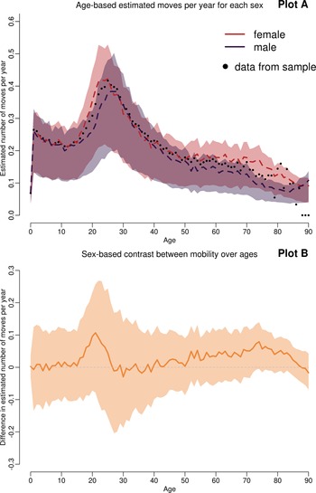
We can specifically address the age-based differences in mobility by simulating from the posterior. The prediction utilises β agei,genderi, the age-based offset, and μ, the general offset, as well as the variation among individuals in mobility tendency. The result of this simulation for each gender is visualised in Figure 3 plot A.

Figure 3. Plot A shows the 50% percentile interval (colour band) of moves per year per age as estimated with β, μ and the distribution of individual effects for both genders (red for females, purple for males). Dashed line denotes mean numbers of moves per age from model, for respective gender. Black circles are mean numbers of moves per age from sample. Plot B shows the contrast between genders in moves per age, with dashed line denoting 0 = no difference. Positive deviations from 0 indicate more female mobility, negative deviations denote more male mobility.
Figure 3 plot A indicates the expected number of moves per year across the lifespan, conditional on attaining each age, from both the model (colour band and dashed line) and sample (black circles). The results show a clear peak in mobility between the ages of 20 and 30, for both females and males. The peak for women is at age 25, with the model estimating 0.42 moves per year at this age (HPDI [0.06, 0.79]). For men, the peak is at age 26, with 0.38 moves per year (HPDI [0.05, 0.71]).
Newborn mobility is an artefact, lower than expected owing to a lack of newborn registrations. Discounting newborns, the lowest mobilities are found in old age. For females, this is at age 87, where the model estimates 0.09 moves per year (HPDI [0.01, 0.17]). For men, the lowest mobility is at age 84, with 0.07 moves per year estimates (HPDI [0.01, 0.14]). For both genders, the difference between peak and trough is just over 30% (33 and 31% for females and males, respectively). Given two counterfactual individuals, each living to 60 years old, with one moving at the mobility of a 25-year-old female their whole life, and the other moving at the mobility of an 84-year-old man, their total lifetime mobility would be 25 and 4 moves, respectively.
Considering gender disparities, Figure 3 plot B shows the contrast between men and women, with positive deviations from zero (grey dashed line) taking place when women move more and negative deviations when women move less than men. Figure 3 plot B suggests that females move more than males in general. In particular, females seem to be much more mobile leading up to their early twenties, moving 10% more than males at age 21. There seems to be very little gender disparity in childhood and only a small male advantage throughout the thirties.
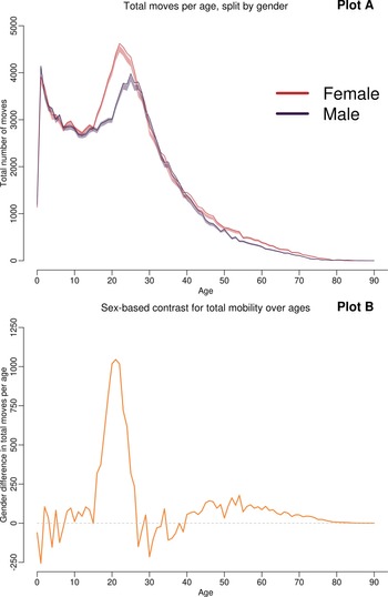
Individual and age-based effects combine to produce the mobility profile observed in the sample. In Figure 4 we plot total moves per age as observed for each gender in the sample (coloured lines, red = female, purple = male) and the predicted total moves per age for each gender from the model posterior, accounting for the age and gender structure of the population. That is, for each observation of the data (a combination of individual, age, and gender), we simulate an estimated number of moves, and sum these across age groups. This post-stratification thus gives us the expected mobility of the population given the age and gender structure of the sample, and allows us to compare the raw data with model outputs.

Figure 4. Plot A shows total mobility events by age for each gender (red for females, purple for males) with the 50% percentile interval of age-based sums of simulated numbers of moves for each observation of the sample. Dark lines denote the mean for each gender from the sample. Plot B shows the contrast between genders in total mobility events by age, with dashed line denoting 0 = no difference. Positive deviations from 0 indicate more female mobility, negative deviations denote more male mobility
Post-stratification is clearly very important here as it carries forward not only the age structure, but also the mortality present in the sample. The shape of the mobility curve suggests that young children move less when age structure is accounted for; there is more children's mobility in Figure 4 than from age-based estimates in Figure 3 because the latter accounts for the steep childhood mortality featured in the sample. Conversely, accounting for population structure does not change the observed gender discrepancy – females tend to move more than males throughout the life course except in their late twenties and throughout their thirties. Accounting for population structure does, however, soften the female advantage in later years, suggesting that differentials in post-reproductive residential mobility are modest but due to mobility propensities.
In both Figure 3s plot A and Figure 4s plot A, the percentile interval is lower than the average data points from the sample; this is due to shrinkage. The statistical model accounts for the fact that the sample features long tails, with few individuals accounting for many moves, and thus the estimated mean is lower (shrunk) in relation to the empirical mean. This is a common feature of long-tailed samples (Efron & Morris, Reference Efron and Morris1977).
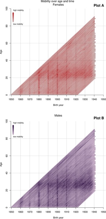
As the sample interrogated here spans almost a century, we conduct a cohort analysis to check that the age-based pattern that we discuss above is consistent through time and is not an artefact of cohort imbalances in the data (Supplementary Information 10.2). We fit the model to birth year subsets of the data, comprising 73 cohorts from birth year 1850 to birth year 1922. Figure 5 shows the age-specific expected mobility for each of these cohorts for each gender. Figure 5 plot A and B suggests that the peak in mobility between ages 20 and 30 is stable through the observed period (reflected by the darker coloured cloud) for both genders. Likewise the gender difference, with females moving more earlier in their twenties, is stable across the cohorts.

Figure 5. Heatmap of moves per year for 73 model runs fit to birth year subsets of data. Females in plot A and males in plot B. Each diagonal represents a birth year-based model fit, showing how a research person born that year would move through time, until 1945, which is when observation records end. Rows allow for observation of the age-based pattern for all model fits while columns allow for an interrogation of cohort effects. Squares are coloured by simulated average number of moves per year of age as in Figure 3; darker colours represent higher mobility
Columns of high mobility reflect heaping at decadal years. Decadal years were census years in the Netherlands and can thus represent an updating of records to reflect the situation witnessed at the census. It remains a challenge for future analyses to statistically redistribute these decadal counts over the previous years, as they did not all happen in the indicated year.
4. Discussion
Our results provide a picture of total residential mobility as experienced by individuals living in a system of permanent settlements in nineteenth- and twentieth-century Netherlands. Our methodology allows us to robustly decompose mobility into individual and age-based effects, while stratifying by gender. The sample shows variation in how residential moves pattern over individuals’ life courses, with a peak in early adulthood, which while present for both genders shows that women moved more in general and particularly earlier in their twenties and then marginally less than men throughout their thirties. We also separate these effects from the population structure, ensuring flexible post-stratification. Our results show the need to account for the composition of the population when inferring population-level mobility regimes, as childhood mortality in particular changes the age-based effect. Our sample comes from a particular region and range of years. Therefore we should not hastily generalise the overall pattern. Still, the amount of data and the unusual ability to analyse individual lifespans is of value for theorising mobility and human adaptation.
The distribution of total residential mobility in the HSN shows that the population is not immobile and there is a long tail of hyper mobile individuals of both genders. We found a median of 10 residential moves per lifetime, with little difference between women and men in terms of total mobility. While it would be necessary to interrogate marital status to check, it is likely that residential mobility is a family affair and thus gender stratification is unproductive, particularly when averaging over the entire life course.
While 10 moves is far below that of highly mobile hunter–gatherer populations, it is by no means an absence of mobility as per the categorisation of a sedentary population. Also, moves may be under reported in the HSN. Even though individuals were legally obliged to report changes in address, human forgetfulness means that mobility is likely to be higher than reported (Adams et al., Reference Adams, Kasakoff and Kok2002).
The range of moves, from 0 to 130 over the lifetime, implies an average of between 0 and 2.6 moves per year over the length of an average lifespan of 50 years, with most individuals having a move every 3 years, as corroborated by the individual-based effects. Comparatively, this puts the historical Dutch at a similar mobility to the Yurok (0–2 moves per year; Kelly, Reference Kelly2013). This comparison of arbitrary categories raises questions about how to meaningfully compare the mobility of societies that occupy different socio-ecological circumstances. While the contrast is stark if we take a historical Dutch population and a contemporary but marginalised hunter–gatherer population, the point is valid for all societal comparisons. That is, the difficulty of this comparison stems from our assumption that mobility functions differently in a modernising society, and means that comparisons between hunter–gatherers on a point estimate are somehow more valid than comparisons between societies with different ecological foundations – a point we should be sceptical of given the known diversity of hunter–gatherer populations (Kelly, Reference Kelly2013; Mattison & Sear, Reference Mattison and Sear2016). This problem is not unique to the evolutionary human sciences. Bernard et al. (Reference Bernard, Forder, Kendig and Byles2017) estimate a ‘complete migration rate’, and suggest that it can be used to compare across countries. By describing the entire distribution of mobility, we hope to emphasise the inadequacy of describing mobility regimes with point estimates, particularly means given the shape of the distribution. It is necessary to develop better ways through which to characterise what we actually mean by high vs. low mobility, and how concepts like sedentarisation and high mobility fit theoretically when broader economic transitions are considered, and when mobility regimes in the global context are compared.
The long tail of the studied mobility distribution, as portrayed by Figure 2 and individual-based effects (Supplementary Information 10.5), suggests a role for high-mobility individuals of both genders, even in populations which show low average mobility. Further work could elucidate whether these individuals, like those studied by Clark (Reference Clark2018), are pursuing high residential mobility as a means to adapt to adverse circumstances in early life. Similarly, previous work on the HSN data provides evidence of the high residential mobility of poor urban dwellers (Kok et al., Reference Kok, Mandemakers and Wals2005). Kok et al. (Reference Kok, Mandemakers and Wals2005) suggest that residential mobility was a means for poor inhabitants to adapt, with residential mobility fluctuating with the rental supply. Given that poor residents could save rent by moving residence (as a means for apartment owners to attract renters), poor residents could be opportunistic and quickly adapt to the changing housing market (Kok et al., Reference Kok, Mandemakers and Wals2005).
Kok et al. (Reference Kok, Mandemakers and Wals2005) study raises questions about the spatial distribution of high mobility individuals, highlighting that urban settlements may be the geographic locus of high mobility. More recent work with contemporary urban populations corroborates this point (e.g. Gillespie, Reference Gillespie2017). As such, future work should explicitly address the geography of residential mobility to see where particular mobility is clustered, and start to address the ecology of high vs. low mobility. This would go a long way in theoretically advancing our understanding of mobility in permanent settlement systems. However, future work must consider that, as Jennings and Gray (Reference Jennings and Gray2015) point out, urban centres are over-sampled in the HSN (Jennings & Gray, Reference Jennings and Gray2015). Thus, if urban settlements have particular mobility signatures, we may find these over represented in the HSN.
Residential mobility varies over the life course, with a peak in early adulthood for both genders. In relation to mobility and age, our study demonstrates that in the HSN, the peak in residential mobility occurs between the ages of 20 and 30, a lesser peak takes place in early childhood, while teenage years and years after 40 represent decreases in residential mobility for both genders. The pattern we find qualitatively resembles the pattern found in Gillespie (Reference Gillespie2017), who explores the 2014–2015 Current Population Survey in the USA, as well as a study of migration in Finland, which utilises the FinnFamily register dataset (1970–2012) (Ghosh et al., Reference Ghosh, Berg, Bhattacharya, Monsivais, Kertesz, Kaski and Rotkirch2018). Both of these studies reproduce the age pattern, indicating that this pattern may hold in a variety of industrialised settings, both current and historical. Although both studies report mobility as a percentage of adults of particular age that are moving (Ghosh et al., Reference Ghosh, Berg, Bhattacharya, Monsivais, Kertesz, Kaski and Rotkirch2018; Gillespie, Reference Gillespie2017), our Gaussian process approach allows us to directly estimate age differentials in moving propensity. This direct estimation also allows us to decouple the age structure from the age effect. When we account for childhood mortality, the peak in early childhood lessens. This post-stratification highlights how mobility regimes are built up from the demographics of the population. As such, even societies with the same age-based pattern may have very different total mobilities, if they differ in their demographic composition. Comparing mobility regimes of different populations without taking stock of their demographic composition is likely to lead to mischaracterisation. Moreover, our decomposition allows for straightforward integration with research on life history, such as comparing with daily expenditures (Pontzer et al., Reference Pontzer, Yamada, Sagayama, Ainslie, Andersen, Anderson and Speakman2021), knowledge accumulation (Koster et al., Reference Koster, McElreath, Hill, Yu, Shepard, Van Vliet and Ross2020), and relatedness to camp-mates through the life course (Dyble et al., Reference Dyble, Migliano, Page and Smith2021).
We stratify our results by gender, and find that while the mobility pattern over the life course is present for both women and men, there are some gender discrepancies. Our results suggest that women move marginally more than men throughout their lives, apart from their thirties. The peak in female mobility is earlier – women move substantially more than men in their early twenties, while men move more than women in their thirties. Given that this period coincides with family formation, the results suggest that women's mobility is penalised more than men's after starting families.
Several researchers of the HSN make a general point about mobility declining after marriage (Adams et al., Reference Adams, Kasakoff and Kok2002; Kok et al., Reference Kok, Mandemakers and Wals2005). Given that young children do not move on their own and our analysis suggests a moderate peak in early life, our results indicate high residential mobility for young families. The moves experienced by young children match those experienced by adults between 30 and 40 (Figure 3). Given that during the study period, the mean age at marriage in the Netherlands dropped from above 27 in 1860 to just under 23 in 1970 (Karel et al., Reference Karel, Vanhaute and Paping2011), it is not difficult to imagine a relatively large group of RPs moving before having children well into their twenties, accounting for the higher peak between 20 and 30. Moreover, given that moves per year then drop off, Adams et al.'s (2002) argument that more children mean less mobility is plausible, and our research suggests that this is particularly true for women.
Recent work with a contemporary Swiss population suggests that higher income is a mitigating factor in allowing individuals to adjust their residence to changing family structures (Lacroix et al., Reference Lacroix, Gagnon and Wanner2020). As such, in the HSN data, the mobility between 20 and 30 may indicate adjustments to housing for a growing family that are either satisfied or can no longer be financed later on in life. Better than postulation, however, would be a direct test. The HSN contains information on household structure, and thus these questions could be resolved with a detailed analysis of household structure, over age, combined with residential mobility.
Our results also suggest women move marginally more than men later on in life, particularly after their forties. It is possible this later mobility reflects ‘mobile grandmothers’ moving to provide help, as documented in the anthropological literature (Jones et al., Reference Jones, Hawkes, O'Connell, Hewlett and Lamb2005). It is important to emphasise that our results are not directly comparable with the literature on gender differences in mobility that exists in the evolutionary community. While we address residential mobility, most of the literature concerns travel behaviour. Without a holistic theoretical account that envisions how these two mobilities relate, it is impossible to compare them. Likewise, we have to stress that our results do not indicate causal effects of age nor of gender. Efforts are being made in the migration literature to connect internal and international migration (King et al., Reference King, Skeldon and Vullnetari2008). Likewise, in evolutionary approaches, we need efforts to synthesise different mobilities and understand how they relate to lifeways, ecologies and culture.
We provide a cohort perspective to asses the stability of the age-based pattern over time (Figure 5). The cohort analysis was intended as a basic assumption check to make sure the age-based pattern was not a feature of differentials across cohorts. The results suggest that the peak in mobility experienced by individuals between their twenties and thirties is stable over the study period. Likewise the gender disparity of the peak of mobility for women and men is reproduced in the cohort analysis, and stable for each of the cohorts addressed.
The cohort result is striking given the scope of change occurring in the Netherlands at this time, with industrialisationand changing agricultural lifeways, as well as population growth (Karel et al., Reference Karel, Vanhaute and Paping2011). The cohort analysis, as visualised in Figure 5 suggests a significant drop in all age classes around the advent of World War II (the Netherlands were invaded in 1940). This observation provides a confidence check for the cohort analysis. However, the age-based mobility pattern holds throughout other periods of turmoil such as World War I and the ensuing deep recession that affected the Netherlands from the 1920s and through much of the 1930s.
This cohort stability, and a reproduction of the same age-based pattern as found in contemporary industrialised populations (Ghosh et al., Reference Ghosh, Berg, Bhattacharya, Monsivais, Kertesz, Kaski and Rotkirch2018; Gillespie, Reference Gillespie2017), raises questions about the extent, depth and origin of the age-based pattern. However, work with the HSN by Bras et al. (Reference Bras, Liefbroer and Elzinga2010) suggests that pathways to adulthood homogenised over the study period, preferring early family formation. As such, regardless of population growth and modernisation, it is possible that this stabilisation is reflected in the consistent mobility pattern we describe. Future work explicitly unpacking family planning and mobility could shed light on the origins of the age-based pattern we described.
We must exercise caution when interpreting the cohort results. It is possible that, given we take a national view, regional variation changes over time but averages out, and cannot be observed at the national level. Also, our results illustrate decadal heaping in registered moves. Given that decadal years were census years, we can view these heaps as times when records were ‘caught up’. However, an analysis particularly focusing on cohort effects would need to treat this heaping statistically. For our aims, however, the stability over cohorts allows us to conclude that discrepancies between the cohorts in terms of representation are not driving our result, providing a control for cohort effects.
To conclude, we have quantified the life course of mobility for a historical Dutch population, showing an age-based pattern that is stable over more than 50 years of dramatic change occurring through the nineteenth and twentieth centuries. Moreover, our results indicate wide individual variation both in the total number of residential moves individuals have over a lifetime as well as the trajectories through life of when they engage in moves. Conversely, our results document stability in the age-based pattern for both genders, with discrepancies that indicate that women move more, and peak in their mobility earlier in life. Our results indicate a disconnect between mobility and the settlement landscape, showing that even when settlements are fixed, people can move and of course do so. We think this study demonstrates the potential of studying adaptive mobility in systems of sedentary and permanent settlements.
Given that our results are possible only due to the high resolution of the HSN sample, we hope that our work stimulates further interest in the HSN sample in the cultural evolution and human behaviour community. Large, high-resolution databases make it possible to test more detailed models of human behaviour, both at individual and population scales. Many anthropological hypotheses are not practically testable in archaeological contexts nor among mobile foragers, because of the poor data resolution or the highly selected nature of the samples. Historical and contemporary data on urban mobility provide an attractive opportunity to develop and refine models of adaptive decisions in built environments. Refined models could then be applied with greater confidence to contexts with lower data resolution.
If theories of human mobility are to be adequately developed and tested, it is a necessary step to rigorously describe high-resolution mobility data. The computational challenges involved in this work are substantial. With small samples, and poor coverage, statistical and theoretical models are necessarily coarse. Yet as databases grow in size, it makes it possible to attend to features like individual trajectories and interactions between demography and movement. This means, however, that the models are more complex and require more computational power and care in construction. Yet new algorithms make it practical to perform high dimensional modelling of these databases. Here we employed Hamiltonian Monte Carlo, which allowed us to estimate individual life trajectories for tens of thousands of historical individuals, as well the populations patterns of these trajectories, without positing any rigid model of age-related patterns. This can be done without traditional fears of overfitting, because the modelling approach, like most machine learning approaches, is built with this problem in mind.
Acknowledgements
We would like to thank the curators of the HSN database at the International Institute of Social History for creating the HSN. Likewise, we are grateful to the EHBEA 2019 community, that provided feedback on a poster presentation of an earlier version. We would like to thank the department of Human Behavior, Ecology, and Culture at the MPI EVA for stimulating discussions and ethnographic comparisons that helped shaped this project, and specifically N.-Han Tran for her input on the statistical model. Finally, we thank Brian Wood and an anonymous reviewer for their helpful feedback.
Author contributions
NF designed the study, performed the analyses, and wrote the manuscript. NF and BAB designed the data processing and analyses. RM provided feedback on the manuscript and analyses. BAB and RM helped shape the research project, analysis, and manuscript.
Financial support
The described research project was supported by the Max Planck Institute of Evolutionary Anthropology.
Conflict of interest
The authors declare that there is no conflict of interest.
Research transparency and reproducibility, and data availability
The data management, analysis, and plotting code is available on GitHub (https://github.com/Naty-fedorova/Dutch-historical-mobility). The data that support the findings of this study are available from the International Institute of Social History, Amsterdam (https://iisg.amsterdam/en/hsn). Restrictions apply to the availability of these data, which were used under licence for this study. To aid with code analysis, structurally comparable simulated data is produced in the repository. Data are available from the corresponding author with the permission of the curators, as is the code required to process the data for analysis.
Supplementary material
To view supplementary material for this article, please visit https://doi.org/10.1017/ehs.2022.33.


 Open access