


1 Introduction and overview
In engineering system design, designers make decisions and take corresponding actions (operations) on design artifacts in a sequential and iterative manner (Miller, Yukish & Simpson Reference Miller, Yukish and Simpson2018). Effective sequential design strategies help to reduce unnecessary design operations (Smith & Eppinger Reference Smith and Eppinger1997) and minimize potential design flaws, thereby improving design efficiency. So, knowledge transfer of such beneficial strategies is of great interest to train novice designers and to the creation of computer agents to imitate human designers for generating feasible design solutions and enable human–AI design collaboration. In either case, in order to extract and integrate human design strategies, computational modeling of sequential design decisions is the key.
Despite its great importance in many facets of design research, the study of human sequential decision-making is challenging because decisions are hidden, implicit and sometimes tacit (Brockmann & Anthony Reference Brockmann and Anthony1998). To fundamentally understand designers’ sequential decision-making strategies, two essential elements in a design process must be considered: design problem (i.e., the artifact to be designed) and designer (Cross & Roy Reference Cross and Roy1989). A well-defined design problem typically outlines the design space where designers can search for the solutions. The search is realized by actions/operations taken on the design artifact, such as adding/deleting a component and modifying the values of corresponding design variables. A designer, on the other hand, is the entity who actually makes design decisions guided by his/her own design thinking and system thinking (Greene, Gonzalez & Papalambros Reference Greene, Gonzalez and Papalambros2019) that are often influenced by prior knowledge and experience. Based on the response to the present action taken (e.g., whether adding a component violates the design constraints or not) as well as the present resources (e.g., current budget), a designer will make the next decision to navigate through the design space searching for acceptable solutions. Therefore, to successfully model a designer’s sequential design decisions, two classes of information must be acquired – the sequential actions (a decision is a commitment to an action (Hazelrigg Reference Hazelrigg2012)) taken by a designer and the designer-related attributes that often form his/her design thinking and system thinking. In this paper, we treat those sequential actions as dynamic data because actions performed at different time steps are different and those designer-related attributes as static data as they often do not change during the period when the design is performed.Footnote 1
However, even if existing work has used sequential design actions (i.e., dynamic data) to computationally model and study designers’ sequential decision-making, for example, with the Markov Model and the Hidden Markov Model (HMM) (Gero et al. Reference Gero, Kan and Pourmohamadi2011; McComb, Cagan & Kotovsky Reference McComb, Cagan and Kotovsky2017b) (see Section 2 for details), we are aware of little research incorporating static data into the modeling. We believe part of the reason could be the difficulties of obtaining such information due to privacy issues. For example, in a design department of a company, while designers’ operations (e.g., modification of codes) can be automatically logged, employees’ demographics are typically not collected or not allowed for research purposes. A more important reason is that it is not clearly known what exact designer-related attributes are useful and how such information can be used in support of the computational modeling of a designer’s sequential decisions.
The research objective of this paper is to combine both static and dynamic data in modeling and predicting human sequential design decisions. To achieve this objective, this paper presents a deep recurrent neural network (RNN) based approach to predict a designer’s future design sequence by combining both sequential data of design actions and static data reflecting designers’ sequential design behavioral patterns. Specifically, we introduce two methods to realize such a combination. In the first method, both static and dynamic data are directly taken as inputs for a typical RNN architecture. In the second method, static data is passed into a feed-forward neural network (FNN) and dynamic data is separately passed into an RNN in the first place. Then, the outputs from the RNN and the FNN are concatenated (a way of combination with matrix operation introduced in Section 4) before the final model output is generated (see Figure 3 for details). It is worth mentioning that this method is a new method developed from this study that is different from the second method that is mostly seen in existing literature. These two methods are tested with two RNN variants: long short-term memory (LSTM) and gated recurrent unit (GRU). The proposed approach and methods are demonstrated in two case studies on solar energy system design, i.e., energy-plus home design and solarized parking lot design.
The scope of the research is focused on the design decisions made in a CAD process for the ease of data collection, but our approach is generally applicable in any design situation as long as designers’ sequential action data can be collected. Since the design is conducted in a CAD environment, the dynamic data refers to the sequence of CAD operations and the static data refers to any information or attributes pertaining to designers who operate the CAD. In both case studies, the  $k$-fold cross-validation method is adopted for model validation. In order to evaluate the models’ predictive performance, both prediction accuracy (percentage of corrected predictions) and the area under the receiver operating characteristics curve (AUROC) (Fawcett Reference Fawcett2006) are adopted (see Section 5.1 for details). In this paper, four models (2 combination methods $\times$ 2 RNN models) are compared in each case study. We hypothesize that by integrating the static information, the prediction accuracy can be improved. The benchmark is therefore the models’ counterpart without including the static data.
When implementing the proposed approach, in order to address the challenges in collecting static data (e.g., designers’ demographics), we devise a novel method that leverages clustering techniques to first cluster designers with similar sequential design behaviors and then use the resulting cluster categories (i.e., cluster indexes) as a proxy of static information for modeling. There are several advantages of doing this. First, the cluster information contains an aggregate-level feature that implicitly combines the effects of many designer-related attributes. For example, designers with similar education backgrounds and ages are more likely to be clustered together. Therefore, this helps avoid diving into the investigation of what static information shall be added to best capture a designer’s thinking, which itself could be a research question. Second, from the methodological point of view, this treatment is essential to use unsupervised learning (i.e., the cluster methods) to produce additional features that can potentially enhance the performance of supervised learning (i.e., the RNN model) for predicting human decisions. This is especially useful to predict design decisions in the system design context, where usually weak behavioral patterns exist in that different designers may have different design strategies and the set of design actions to be taken vary at different design phases (e.g., conceptual design and parametric design) that often span a long period. Third, this treatment can help alleviate a major conflict in design research that involves human subjects as it often suffers from a shortage of subjects, meaning a lack of large-scale data for deep learning.
The remaining paper is organized as follows. In Section 2, a literature review on the studies of sequential decision-making in engineering design is presented. We also review state-of-the-art deep-learning models that use different methods to combine static and dynamic data in the disciplines beyond the engineering design field. In Section 3, a technical background of the RNN is provided, which is followed by the proposed research approach. Section 4 presents the two case studies. In Section 5, the results are presented, the models are compared and the pros and cons of each model and method are discussed. Finally, in Section 6, we conclude our research with closing thoughts and provide the future direction of the study.
2 Review of relevant literature
2.1 Sequential decision-making in engineering design
In the engineering design field, designers’ sequential decision-making is primarily studied with probabilistic models. Among them, the Markov Chain (MC) model and the HMM are considerably used for understanding sequential design behaviors and identifying design patterns. For example, in configuration and parametric design problems, first-order MC models have been used to extract frequently occurring pairs of design actions (Yu et al. Reference Yu, Gero, Ikeda, Herr, Holzer, Kaijima, Kim and Schnabel2015) and study designers’ sequential learning process (McComb et al. Reference McComb, Cagan and Kotovsky2017b). Rahman et al. (Reference Rahman, Gashler, Xie and Sha2018) also combined different clustering methods with the MC model to identify sequential design behavioral patterns. In other studies, second-order MC is implemented in a design tool, called LINKOgrapher, to compare the design processes between architects and software designers (Gero et al. Reference Gero, Kan and Pourmohamadi2011), and higher-order MC models are adopted in an agent-based modeling framework to study the effect of memory on sequential behaviors (Kan & Gero Reference Kan and Gero2009). Using the HMM, McComb, Cagan & Kotovsky (Reference McComb, Cagan and Kotovsky2017a) identify four general hidden states on the basis of two configuration design problems, where the first two hidden states are topological operations, the third state is about spatial operations, and the fourth state is related to parameter operations. In a later study, Raina, McComb & Cagan (Reference Raina, McComb and Cagan2018) show how human design strategy can be extracted by HMM to create and augment computer agents to solve a truss design problem. The team also shows that design strategies can be successfully transferred to a similar design problem, which requires less time to complete the design task.
In addition to MC and HMM models, other stochastic methods are also utilized to develop sequential decision models. In order to understand human design strategies during the sequential information acquisition decision-making, the Gaussian Process is used to develop a probabilistic decision model of choosing design parameters and stopping design searches (Chaudhari & Panchal Reference Chaudhari and Panchal2019). Sha, Kannan & Panchal (Reference Sha, Kannan and Panchal2015) and Panchal, Sha & Kannan (Reference Panchal, Sha and Kannan2017) integrate the Gaussian Process with a non-cooperative game-theoretic model to understand human sequential design behaviors under competition and the trade-off decisions between design cost and design quality. In a vehicle design problem, Bayesian Optimization is used as a computational framework to mimic human solution-searching strategy, and it is observed that the model performance can be improved when the parameters are learned from a human’s effective searching strategies (Sexton & Ren Reference Sexton and Ren2017).
Other optimization techniques and theoretical models, such as the design structure matrix (Yassine Reference Yassine2004), multi-objective optimization (Miller, Simpson & Yukish Reference Miller, Simpson and Yukish2017), expected value of perfect information (Griffin, Welton & Claxton Reference Griffin, Welton and Claxton2010), genetic algorithm (Meier, Yassine & Browning Reference Meier, Yassine and Browning2007), and optimal learning (Duff & Barto Reference Duff and Barto2002), have been also used to study the optimal design sequences. However, they cast the design problem into a sequential decision process to be optimized with normative models. They do not study the sequential decision-making of human designers. In the above studies on human sequential decision-making, either the models are trained for predicting or the model parameters that characterize design strategies are estimated for an explanation of observed design behaviors; the input data used are dynamic data only, e.g., the sequential data of design actions taken at each time step. No static data of designers’ attributes and characteristics are utilized.
2.2 Using recurrent neural network to model sequential data
The emerging success of deep-learning algorithms has brought a revolutionary breakthrough in various engineering and science fields in recent years (Deng & Yu Reference Deng and Yu2014). The RNN, one of the deep-learning models, is particularly effective for handling sequential or dynamic data for machine learning. For example, Almeida & Azkune (Reference Almeida and Azkune2018) propose a deep-learning architecture based on the LSTM, a variant of RNN, to predict users’ future activities during a day, such as sleeping, walking, and eating, with sensor data collected from wearable devices. The model can successfully predict a user’s next action and help identify anomalous behaviors.
While predicting future events, the majority of the RNN-based models merely utilize dynamic data. There are only a few studies that use both static and dynamic data for prediction by leveraging a separate algorithm, such as the FNN or random forest model. For example, Esteban et al. (Reference Esteban, Staeck, Baier, Yang and Tresp2016) present a deep-learning approach that takes static information (i.e., gender, blood group) into an FNN and dynamic information (patients’ visits at different times) into an RNN to predict future clinical events. The model is applied to the data collected from kidney failure patients and predict among three possible endpoints that would occur after kidney transplantation. In a similar study (Makris et al. Reference Makris, Kaliakatsos-Papakostas, Karydis and Kermanidis2017), but in musical research, a deep-learning architecture is developed by combining LSTM and FNN to generate drum sequences. In this architecture, drum sequences, i.e., the dynamic data, collected from three bands, are fed into an LSTM layer while the FNN takes the bass information as static data. The outputs of both layers are then merged to produce the final sequence. To automatically recognize hand-written digits, Sharma (Reference Sharma2015) extracted static data and dynamic data from digit images. The static data includes white in a square, i.e., a horizontally, vertically and diagonally divided region in the pixel. The dynamic features are extracted from the drawing order of the corresponding image of the digit. The support vector machine is used to classify the digit with these concatenated sets of features for the recognition of hand-written digits.
Table 1. Comparison of the studies that combine static data and dynamic data

Table 1 shows the summary of the studies that use both static and dynamic data in the deep-learning methods. But none of them is related to engineering design. More importantly, there are some fundamental differences between the existing studies and the present work, particularly in the following three aspects.
(i) There could be a large number of design actions and the actions can be different types in engineering design problems. On one hand, this causes high-dimensional text data, which challenges the modeling and deep learning. On the other hand, each action is chosen by the designers and thus reflect their thinking/objectives the moment when they made such a choice. This feature requires the knowledge of an appropriate design process model to abstract the design action to the level of the design process in order to better study human design thinking and behaviors.
(ii) The complexity associated with the sequential data in engineering design is more than that of the data handled in the existing literature. For example, in Esteban et al. (Reference Esteban, Staeck, Baier, Yang and Tresp2016), each data in the sequence represents one of the three endpoints that a kidney patient may face after kidney transplantation, i.e., kidney rejection, kidney loss and death of the patient. The inputs are laboratory analysis results obtained at different dates. Such sequential data are objective values and do not indicate any human thinking. Thus they do not require a meta-model of design thinking for characterization.
(iii) In engineering design, while design actions can be automatically logged from tools that designers interact with, their demographic information and attributes are often not collected or very limited. This is different from the existing literature, for example, in the application of clinical events, patients’ information can be readily obtained because their personal information needs to be provided at the time of visit. Little study was conducted in the design field that provides a solution to combine both types of data for the prediction of sequential design decisions. There is a knowledge gap that must be filled in order to better facilitate design research where much static information of human factors cannot be neglected.
In our previous study (Rahman, Xie & Sha Reference Rahman, Xie and Sha2019), we developed an approach that integrates the function–behavior–structure (FBS) based design process model and different artificial neural network models, such as LSTM and FNN, to predict designers’ future design process stages in a system design context. The objective of that study was to compare the deep learning-based approach with the models (e.g., MC and HMM) that have been traditionally used in design research to study human sequential decisions. Moreover, our previous study uses dynamic data only for model training and does not combine any static information in the model. So, those models developed in our previous study will serve as the benchmark for evaluating the performance of the models presented in this paper.
3 Technical background and research approach
In this section, we first provide an overview on the technical background of the RNN. Next, we present the approach that combines both designers’ static information and dynamic design process data to model and predict human sequential decisions in engineering design. To realize such a combination, two methods are developed and these methods are introduced in Sections 3.2.2.
3.1 Technical background of recurrent neural network

Figure 1. The structures of RNN, LSTM, and GRU.
The RNN is a class of deep neural networks, which consist of artificial neurons with one or more feedback loops (Lipton, Berkowitz & Elkan Reference Lipton, Berkowitz and Elkan2015) designed for pattern recognition in sequential data. A typical RNN consists of three layers: an input layer, a recurrent hidden layer, and an output layer. The feedback loop in the recurrent hidden layer enables the RNN to keep the memory of past information. Figure 1(a) shows a standard RNN structure. Given a sequential data with  $T$ time steps $\{\boldsymbol{x}_{1},\ldots ,\boldsymbol{x}_{t},\ldots ,\boldsymbol{x}_{T}\}$, at time step $t$, the hidden state of the RNN is computed by
 $$\begin{eqnarray}\boldsymbol{h}_{t}=f_{\text{RNN}}(\boldsymbol{h}_{t-1},\boldsymbol{x}_{t}),\end{eqnarray}$$
 where  $\boldsymbol{x}_{t}\in \boldsymbol{R}^{N}$ is the vector of the $t$th input; $\boldsymbol{h}_{t-1}\in \boldsymbol{R}^{M}$ is the hidden state of the last time step. Hence, by taking the previous hidden state $\boldsymbol{h}_{t-1}$ and the up-to-date information $\boldsymbol{x}_{t}$ as the input, at each time step, the hidden state $\boldsymbol{h}_{t}$ encodes the sequence information up to $\boldsymbol{x}_{t}$. Then, given the hidden state $\mathbf{h}_{t}$, the output layer is computed as
 $$\begin{eqnarray}\hat{\boldsymbol{y}}_{t}=g(\boldsymbol{W}_{O}\boldsymbol{h}_{t}+\boldsymbol{b}_{O}),\end{eqnarray}$$
 where  $\hat{\boldsymbol{y}}_{t}$ is the predicted output at the $t$th step. $\boldsymbol{W}_{O}\in \boldsymbol{R}^{K\times M}$ and $\boldsymbol{b}_{O}\in \boldsymbol{R}^{K}$ are the model parameters as well, which will be updated during training. $g(\cdot )$ is the output function that adopts the sigmoid function for binary classification and the softmax function for multi-class classification. The objective of the RNN is to make the predicted sequence close to the observed (true) sequence. By using the observed data as the supervised signal, the RNN is trained via backpropagation through a time algorithm (Werbos Reference Werbos1990). However, the classical RNN model suffers from the problem of vanishing gradient (Bengio, Simard & Frasconi Reference Bengio, Simard and Frasconi1994). To alleviate this problem, two variants of the RNN, i.e., LSTM (Hochreiter & Schmidhuber Reference Hochreiter and Schmidhuber1997) and GRU (Cho et al. Reference Cho, Van Merriënboer, Gulcehre, Bahdanau, Bougares, Schwenk and Bengio2014), are proposed by incorporating the gate mechanism.
The LSTM contains special units called memory blocks in the recurrent hidden layer. Each memory block contains an input gate, a forget gate, and an output gate to control the flow of information (see Figure 1(b)). The LSTM uses the following equations as the form of  $f_{\text{RNN}}$ defined in Eq. (1) to compute the hidden state $\mathbf{h}_{t}$:
 $$\begin{eqnarray}\begin{array}{@{}c@{}}\displaystyle \boldsymbol{f}_{t}=\unicode[STIX]{x1D70E}(\boldsymbol{W}_{f}\boldsymbol{x}_{t}+\boldsymbol{U}_{f}\boldsymbol{h}_{t-1}+\boldsymbol{b}_{f}),\\ \displaystyle \check{\boldsymbol{c}}_{t}=\tanh (\boldsymbol{W}_{c}\boldsymbol{x}_{t}+\boldsymbol{U}_{{\check{c}}}\boldsymbol{h}_{t-1}+\boldsymbol{b}_{{\check{c}}}),\\ \displaystyle \boldsymbol{i}_{t}=\unicode[STIX]{x1D70E}(\boldsymbol{W}_{i}\boldsymbol{x}_{t}+\boldsymbol{U}_{i}\boldsymbol{h}_{t-1}+\boldsymbol{b}_{i}),\\ \displaystyle \boldsymbol{c}_{t}=\boldsymbol{f}_{t}\odot \boldsymbol{c}_{t-1}+\boldsymbol{i}_{t}\odot {\check{c}}_{t},\\ \displaystyle \boldsymbol{o}_{t}=\unicode[STIX]{x1D70E}(\boldsymbol{W}_{o}\boldsymbol{x}_{t}+\boldsymbol{U}_{o}\boldsymbol{h}_{t-1}+\boldsymbol{b}_{o}),\\ \displaystyle \boldsymbol{h}_{t}=\boldsymbol{o}_{t}\odot \tanh (\boldsymbol{c}_{t}),\end{array}\end{eqnarray}$$
 where  $\boldsymbol{x}_{t}$ is the input at the $t$ time step; $\odot$ indicates the element-wise product; $\boldsymbol{i}_{t}$, $\boldsymbol{f}_{t}$, and $\boldsymbol{o}_{t}$ are the input gate, forget gate, and the output gate, respectively; $\boldsymbol{c}_{t}$ is the cell state vector; $\boldsymbol{W}$, $\boldsymbol{U}$ and $\boldsymbol{b}$ are the model parameters.
Another variant of the classical RNN is the GRU, which has fewer parameters compared with the LSTM. Figure 1(c) shows a GRU unit. The GRU adopts the following equations as the form of  $f_{\text{RNN}}$ defined in Eq. (1) to compute the hidden state $\mathbf{h}_{t}$:
 $$\begin{eqnarray}\begin{array}{@{}c@{}}\displaystyle \boldsymbol{r}_{t}=\unicode[STIX]{x1D70E}(\boldsymbol{W}_{r}\boldsymbol{x}_{t}+\boldsymbol{U}_{r}\boldsymbol{h}_{t-1}+\boldsymbol{b}_{r}),\\ \displaystyle \boldsymbol{z}_{t}=\unicode[STIX]{x1D70E}(\boldsymbol{W}_{z}\boldsymbol{x}_{t}+\boldsymbol{U}_{z}\boldsymbol{h}_{t-1}+\boldsymbol{b}_{z}),\\ \displaystyle \tilde{\boldsymbol{h}}_{t}=\tanh (\boldsymbol{W}_{h}\boldsymbol{x}_{t}+\boldsymbol{r}_{t}\odot \boldsymbol{U}_{h}\boldsymbol{h}_{t-1}+\boldsymbol{b}_{h}),\\ \displaystyle \boldsymbol{h}_{t}=\boldsymbol{z}_{t}\odot \boldsymbol{h}_{t-1}+(1-\boldsymbol{z}_{t})\odot \tilde{\boldsymbol{h}}_{t},\end{array}\end{eqnarray}$$
 where  $\boldsymbol{r}_{t}$ is the reset gate, while $\boldsymbol{z}_{t}$ indicates the update gate. It decides how much of the previous information shall be kept.
3.2 The research approach
In this subsection, we present the approach that integrates RNNs as well as clustering techniques to combine both static and dynamic data for predicting human sequential design decisions.
3.2.1 Using RNN to predict sequential design decisions
The proposed approach consists of three parts, data preprocessing, data analysis and preparation, and modeling, machine learning & prediction, as shown in Figure 2. In the preprocessing step, we collect raw design behavioral data, which reflect designers’ sequential decisions. The raw data can be collected from different sources such as CAD logs (Gopsill et al. Reference Gopsill, Snider, Shi and Ben2016), design journal of the engineering design process, and documents/sketches generated from thinking-aloud protocol studies (Suwa & Tversky Reference Suwa and Tversky1997). The raw data includes a detailed description of design processes generally including both design actions (or design operations) at each time step and associated values of design parameters at that moment. For example, in this study, we focus on the action taken at each step, such as adding a component, deleting a component or changing the parameters of the components, so that sequential decision information is extracted from the raw data.
With the collected sequential data of design actions, a design process model is applied to convert design actions into particular design process stages. This proposed step is important and necessary for two reasons. First, the design process model generalizes the design actions to understand designers’ behaviors. In the system design task, designers use various design actions, which are actually the reflection of the design-thinking process. Moreover, design actions in different design tasks are different. A design process model at the ontological level (e.g., the FBS model) captures the context-independent essences of design thinking regardless of a particular design task being studied. That helps conduct a better probe into designers’ thought processes and decision-making in system design (Goldschmidt Reference Goldschmidt2014). Second, system design requires a large variety of actions to complete the task. When we want to computationally model these large design actions, it creates a high dimensionality of data. As a consequence, the vectorization of those text data of design actions, e.g., one-hot vectorization, becomes ineffective as the resulting matrix will be very sparse. The design process model at a higher level of description can reduce the dimensionality significantly.
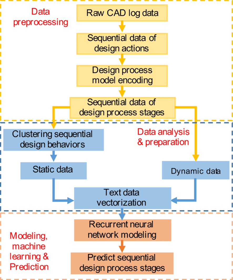
Figure 2. The approach of combining static data and dynamic data in RNN to predict sequential design decisions.
After obtaining the sequential data characterized as design process stages, we adopt the RNN to model the decision-making process and predict the next design process stage that a designer would enter. But before the step of modeling, on one hand, the sequential decision data of design process stages are treated as dynamic data and fed into the RNN. On the other hand, the sequential decision data will be used to cluster designers into different groups, where each group contains the designers sharing similar decision-making behaviors (Rahman et al. Reference Rahman, Gashler, Xie and Sha2018). Each resulting cluster category is an aggregated reflection of the attributes (e.g., knowledge background, age, etc.) of designers in the same cluster that collectively form their cognitive skills and thinking, which, in turn, inform their sequential design decisions. The clustering indexes will be used as the static data input of the RNN. It is worth noting that our approach does not limit researchers to only use clustering information as static data. In this study, we propose to use clustering for generating static data with the motivation of addressing data scarce issues due to limited access to designers’ demographics in regular design activities. Researchers can always append additional designers’ attributes as the static behavioral feature information to further enhance the model performance. Then, both the clustering information and the sequential design process information are used to train the RNN models.
Finally, the trained RNN models will be able to predict the next design process stage that a designer would enter. We consider the prediction of the design process stage as a multi-class classification problem, where each design process stage is a class in our model. We aim to accurately predict the next design process stage given the historical input. The results will be compared and assessed against baseline models through prediction accuracy. In the following subsection, we introduce two methods of combining the static and dynamic data in RNN.
3.2.2 Two methods of integrating static and dynamic data in RNN
First method: Direct input
In the first method, we combine static data with the dynamic data as one single input to the RNN via the concatenation operation. Figure 3(a) shows the structure of the first method. Formally, given a designer  $i$, let $\boldsymbol{x}_{i}$ denote the static data of the designer and $\boldsymbol{x}_{t}$ indicate the design stage at the $t$th step of that designer. The concatenation of the static information and dynamic information is represented as
 $$\begin{eqnarray}\boldsymbol{x}_{t,i}=[\boldsymbol{x}_{t},\boldsymbol{x}_{i}].\end{eqnarray}$$
 To compute the hidden state of the network, we pass  $\boldsymbol{x}_{t,i}$ as the input to the RNN,
 $$\begin{eqnarray}\boldsymbol{h}_{t,i}=f_{\text{RNN}}(\boldsymbol{x}_{t,i},\boldsymbol{h}_{t-1}),\end{eqnarray}$$
 where in our experiments, LSTM or GRU is adopted as  $f_{\text{RNN}}$ to model the user decision-making sequences. Finally, we adopt the $\text{softmax}$ function as the output layer to predict the next design process stage at time step $t+1$. The $\text{softmax}$ function outputs a vector of probabilities for each design process stage. After training, we choose the design process stage with the highest probability as the predicted design process stage. The $\text{softmax}$ function is defined as
 $$\begin{eqnarray}P(\hat{\boldsymbol{y}}_{t+1,i}=k|\boldsymbol{h}_{t,i})=\text{softmax}(\boldsymbol{h}_{t,i})=\frac{\exp (\boldsymbol{w}_{k}\boldsymbol{h}_{t,i}+\boldsymbol{b}_{k})}{\mathop{\sum }_{k^{\prime }=1}^{K}\exp (\boldsymbol{w}_{k^{\prime }}\boldsymbol{h}_{t,i}+\boldsymbol{b}_{k^{\prime }})},\end{eqnarray}$$
 where  $K$ is the number of design process stages; $\hat{\boldsymbol{y}}_{t+1,i}$ is the predicted design process stage of the $i$th user at time $t+1$; $\boldsymbol{w}_{k}$ and $\boldsymbol{b}_{k}$ are the parameters of $\text{softmax}$ function for the $k$th class.

Figure 3. (a) First method: Direct input. (b) Second method: Indirect input.
Second method: Indirect input
In the second method, as shown in Figure 3(b), we use the static and dynamic data separately for the model input. The key idea is to first model the static data through an FNN and the dynamic data through an RNN. Since the hidden states of the FNN and the RNN capture the users’ static information and dynamic design decision data separately, we adopt the concatenation operation to combine the hidden states of both the FNN and the RNN so that the concatenated hidden state encodes both static and dynamic data information. Finally, we adopt the concatenated hidden state to predict the next design stage. Specifically, the hidden state of the static data can be represented as follows:
 $$\begin{eqnarray}\boldsymbol{h}_{i}=f_{\text{FNN}}(\boldsymbol{x}_{i}),\end{eqnarray}$$
 where  $f_{\text{FNN}}$ represents an FNN. The hidden state for the dynamic input is calculated by the RNN:
 $$\begin{eqnarray}\boldsymbol{h}_{t}=f_{\text{RNN}}(\boldsymbol{x}_{t},\boldsymbol{h}_{t-1}).\end{eqnarray}$$
In this method, we combine the hidden states of static and dynamic data via the concatenation operation:
 $$\begin{eqnarray}\boldsymbol{h}_{t,i}=[\boldsymbol{h}_{t},\boldsymbol{h}_{i}].\end{eqnarray}$$
 Since  $\boldsymbol{h}_{t,i}$ captures the hidden information of both static and dynamic data, similar to the first method, we adopt Eq. (7) to predict the next design process stage. In this work, we consider the prediction of the next design process stage as a classification task. Hence, we adopt the categorical cross-entropy method (Goodfellow, Bengio & Courville Reference Goodfellow, Bengio and Courville2016) as the loss function to train the neural networks:
 $$\begin{eqnarray}L=-\frac{1}{N}\mathop{\sum }_{i=1}^{N}\mathop{\sum }_{t=1}^{T}\boldsymbol{y}_{t,i}\log (\hat{\boldsymbol{y}}_{t,i}),\end{eqnarray}$$
 where  $N$ is the number of users, $T$ is the length of the sequence, $\hat{\boldsymbol{y}}$ is the predicted design process stage and $\boldsymbol{y}$ is the actual stage.
4 Predicting sequential design decisions in solar system design – two case studies
In this section, we introduce the design challenges for data collection and data processing procedures for implementing the proposed approach in the context of solar energy system design. The sequential data of design actions are collected from two design challenges. In the first challenge, the task is to design an energy-plus home, while in the second challenge, the task is to design a solarized parking lot at the University of Arkansas. These two design problems exhibit different levels of design complexity (Summers & Shah Reference Summers and Shah2010). For example, the energy-plus home design is more complex in the sense that it has more design variables and more complex couplings between variables than those of the parking lot design problem. Therefore, they are useful in testing the generality of the proposed approach and methods.
4.1 The design challenges
4.1.1 The energy-plus home design and the solarized parking lot design
In the energy-plus home design, the objective is to maximize the annual net energy (ANE) of a home with a budget of $200,000. The problem is well defined, meaning that both the design objective and constraints are given. Note that the conceptual part of this design is still an open problem. Therefore, designers need to go through almost the whole design process from conceptual design to embodiment design, and to analysis and evaluation. Figure 4(a) shows an example of the energy-plus home design accomplished by one of the participants.

Figure 4. Design examples from one participant: (a) energy-plus home design; (b) solarized parking lot design.
In the solarized parking lot design, the context becomes more authentic. Participants are asked to solarize the Bud Walton Arena parking lot at the University of Arkansas, as shown in Figure 4(b). In this design, the objective is still to maximize the ANE, but the budget is $1.5M. Similarly, we provide participants with design requirements. The design requirements of both of the design problems are shown in Table 2.
Table 2. Design requirements of the design challenges

Both design tasks are conducted in Energy3D, a CAD software for solar energy systems, developed by the co-author (Xie et al. Reference Xie, Schimpf, Chao, Nourian and Massicotte2018) and was recently extended to a research platform for design-thinking studies (Rahman et al. Reference Rahman, Schimpf, Xie and Sha2019). Energy3D has several features that are particularly useful for design research. For example, Energy3D logs every design action and design snapshots (the CAD models, not images) at a fine-grained resolution. These data represent the smallest transformation possible on a design artifact. So, the design process can be entirely reconstructed without losing any important details. Energy3D has built-in modules of engineering analysis and financial evaluation that can support the full cycle design of a solar energy system seamlessly. This supports the data collection during both intra- and inter-stage design iterations. Energy3D stores data in a standard data format as JavaScript Object Notation (JSON), which facilitates the postprocessing and analysis. The rich data obtained in time scale is essential to the training of the deep-learning model.
In a JSON file, one action is logged in one line. The information contains the timestamp, the design action and its corresponding parameters such as the coordinates of the object, the ANE output, construction cost etc. The following box shows two lines of data as an example:

4.1.2 The human-subject experiment
The experiment is conducted as a form of design challenge because there is a competition mechanism to incentivize the participants to explore the design space as much as possible. Specifically, the mechanism relates the final reward of a participant to the quality of his/her own design. One design challenge consists of three phases: pre-session, in-session, and after-session. The pre-session lasts about 30 minutes and is designed for familiarizing students with the Energy3D operating environment, the design problem, and basic solar science concepts. The purpose is to mitigate the effect of the learning curve and minimize the potential bias caused by different levels of pre-knowledge of participants. The data generated in the pre-session are abandoned and not used in the case study. During the in-session, participants work on the design problem based on the instruction, including the design statement and the requirements mentioned above. A record sheet is also provided for participants to record the design objective values for feedback and reinforcement of decision-making. The in-session lasts about 90 minutes. The after-session, which lasts about 10 minutes, is for participants to claim rewards and sign out the challenge.
In the energy-plus home design, 52 students from the University of Arkansas participated. The participants are indexed based on their registered sessions and laptop numbers. For example, A02 indicates a participant who was in session A and used laptop #2. On average, each participant spends 1500 actions (CAD operations) to accomplish the task. Some actions, such as adjusting camera view, adding human, that do not essentially affect the design artifact, are removed. With this treatment, each participant uses 335 valid design actions on average among which 115 actions are unique. In the solarized parking lot design, there were 41 participants. After removing trivial actions, each participant uses an average of 350 design actions, among which 72 actions are unique.
4.2 Data preparation and combination of static and dynamic data
4.2.1 Transformation of design action sequence to design process stages

Figure 5. Transformation of the sequential data of design actions to the sequential data of design process stages based on FBS design process model.
After obtaining the raw sequential CAD log data, the design actions, such as ‘Add rack’ and ‘Add solar panel’, are extracted as the sequential data for training the RNN models. As introduced in Section 3.2, a design process model is needed to transform the design action sequence to the sequence of design process stages for better understanding designers’ thinking and decision-making at a higher level of cognition. In this study, the FBS-based design process model (Gero Reference Gero1990) is adopted and the coding scheme in Table 3 is used to categorize each design action into one of the seven design process stages, including Formulation (F), Synthesis (S), Analysis (A), Evaluation (E), Reformulation 1 (R1), Reformulation 2 (R2), and Reformulation 3 (R3). The FBS-based process model is adopted as it is a well-accepted design ontology that can be used universally to represent a system’s design process regardless of the application context (Kan & Gero Reference Kan and Gero2009). Also, it is evident that the FBS ontology well represents design-thinking strategies with its constructs that capture the actions to be taken for achieving design objective and evaluating design performance (Gero & Kannengiesser Reference Gero and Kannengiesser2004). Figure 5 shows an example of one segment of a design sequence from a participant and its transformation to the design process stages after encoding with the FBS model.
Table 3. The FBS model and the proposed coding scheme for design actions (Rahman et al. Reference Rahman, Schimpf, Xie and Sha2019)

4.2.2 Using clustering analysis to obtain static behavioral data
With the sequential data of the design process stages, we perform the clustering analysis to categorize participants into different classes representing different sequential decision-making behavioral patterns. This analysis helps to obtain the static data pertaining to each designer.
In this study, the MC-based approach proposed in our previous study (Rahman et al. Reference Rahman, Gashler, Xie and Sha2018) is adopted for the clustering analysis. As a quick summary, the first-order MC model is applied on each designer’s sequential data to obtain the  $7\times 7$ transition matrix, which is then converted to a $49\times 1$ vector. By combining the transition vectors of all the $N$ participants, we obtain a $49\times N$ matrix that will be used for clustering analysis. In total, we test three clustering methods including K-means clustering, hierarchical agglomerative clustering and network-based clustering, and each method is tested with three options of the number of clusters, i.e., 4, 5 and 6, which are suggested by the elbow plot (Kodinariya & Makwana Reference Kodinariya and Makwana2013). Based on the metric of effectiveness defined in (Rahman et al. Reference Rahman, Gashler, Xie and Sha2018), it is found that for the energy-plus home design dataset, hierarchical agglomerative clustering with 4 clusters performs best while for the solarized parking lot design dataset, network-based clustering with 5 clusters measured performs best. For the details of clustering analysis approaches and their implementation, refer to (Rahman et al. Reference Rahman, Gashler, Xie and Sha2018). Figure 6 shows an example of the results of hierarchical agglomerative clustering with 4 clusters for the energy-plus home design dataset.
The clustering analysis gives every designer an index that is used as the static information to be combined with the dynamic data (i.e., the sequential data of design process stages) for training the RNN models. In the following subsection, we introduce two different methods for realizing such a combination.

Figure 6. Hierarchical clustering of four groups for the energy-plus home design dataset. X-axis label indicates the participants who are clustered together in different colored boxes.
4.2.3 Combining static and dynamic data
Before combining the static and dynamic data for RNN modeling, we transform the static and dynamic text data to one-hot vectors because neural network models cannot work with text data directly. Since the FBS model has already helped reduce the dimensionality of sequential data from the action level to the process stage level, one-hot vector under this circumstance is an appropriate and efficient method to vectorize the data.

Figure 7. The cluster information is added directly to the sequential data of a designer who is in Cluster #2.
In the first method, we combine the static data directly with the dynamic data, as shown in the schematic diagram in Figure 7. In this example, the designer is from cluster 2 (identified by the hierarchical agglomerative algorithm) and its corresponding one-hot vector is appended behind each one-hot coded sequential design process stage. Since the cluster index does not change over time, the same one-hot vectors are appended as long as the sequential data are for the same person. Then, the combined vectors are fed into the RNN layers in the same manner as done by a normal RNN training process.
Different from the first method, the second method allows static data and dynamic data to be processed in separate layers. This means the cluster data and the sequential data are handled separately during the input and are trained by different models, and the resulting outputs from the hidden layer are then combined before sending to the output layer for backpropagation. For example, as shown in Figure 8, the one-hot vector of the cluster index of number 2 is passed as the input of the hidden layer, i.e., an FNN model. At the same time, the one-hot encoded sequential data are passed as the input of the hidden layer, i.e., an RNN with LSTM layers. Then, the results from both the FNN layer and the LSTM layer are combined and then passed to the output layer for training.

Figure 8. Combining the cluster data into the sequential data in separate layers. Cluster data are the input of an FNN layer and sequential data are the input of an LSTM layer.
With both methods, we train the models and then use the trained model to predict the next design process stage. In the following section, we compare the results of the prediction accuracy from both methods. We also perform the sensitivity analysis to investigate how the prediction accuracy would change with different model configurations and experimental settings.
5 Model implementation and evaluation
In this section, we first present the model setup and the method of evaluating the models’ predictive performance. Then, the results are of the prediction accuracy for both methods in two case studies are presented and discussed.
5.1 Mode setup and evaluation method
Baseline: The RNN models that use the sequential data of design process stages only without using static data are chosen as the baseline model for comparison and evaluation.
Cross-validation: We conduct  $k$-fold cross-validation (Yadav & Shukla Reference Yadav and Shukla2016) to evaluate the performance of the models. In the $k$-fold cross-validation, the dataset is split into $k$ partitions, $\{C_{1},C_{2},\ldots ,C_{k}\}$, where $k$ is the total number of validation folds. Then, $k$ rounds of training and testing are performed in a way that in each iteration the model is trained on partitions $\{C_{1},\ldots ,C_{i-1},C_{i+1},\ldots ,C_{k}\}$ and evaluated on the $C_{i}$ partition. In this study, we adopt the 4-fold cross-validation technique to evaluate the models. In order to split the dataset into 4 folds, two different split procedures are used as there are two different data combination methods. In the first method, we directly add cluster information to the corresponding designer’s sequential data. Then we split each dataset into 4 folds. In the second method, we split both the sequential data and cluster data into 4 folds, separately.
Hyperparameter: In order to find the best hyperparameter settings of the RNN models for training, we trial and error different settings and choose the best one to measure the accuracy. As we compare those models with the baseline models, we run different settings on the sequential data without combining the cluster information first in order to obtain the best configuration. Then, these settings are adopted in the models combining both static and dynamic data for a fair comparison.
We implemented the models using LSTM and GRU, respectively. The dimension of the hidden layer is 256. To prevent overfitting, we use 20% dropout regularization (Srivastava et al. Reference Srivastava, Hinton, Krizhevsky, Sutskever and Salakhutdinov2014). We trained each of the settings for 50 epochs although after 30 epochs the accuracies are not significantly improved. Adaptive moment estimation (Adam) is adopted as the stochastic optimization algorithm for the estimation of parameters in backpropagation (Kingma & Ba Reference Kingma and Ba2014). The computation is performed with the Keras deep-learning library (Chollet Reference Chollet2018).
The metrics for predictive performance: As previously mentioned, we get the prediction of the  $t$th design process stage using the previous $t-1$ design process stages. Therefore, for a design sequence with $n$ actions, the model will produce $n-1$ predictions. These predictions are compared with the observed data, and the total number of correct predictions $(n_{i}^{\text{cp}})$ can therefore be obtained. The prediction accuracy can be therefore defined in Eq. (12) by averaging the scores from each round of the cross-validation.
 $$\begin{eqnarray}\text{Prediction Accuracy}=\frac{1}{R}\mathop{\sum }_{i=1}^{R}\left(\frac{n_{i}^{\text{cp}}}{n_{i}^{\max }-1}\right),\end{eqnarray}$$
 where  $R$ is the number of rounds (i.e., iterations) in the cross-validation and $n_{i}^{max}$ is the length of the longest design sequence in the round $i$. In this paper, only the prediction accuracy of the testing data (i.e., the testing accuracy) is reported. To account for the uncertainties, we conduct 4-fold cross-validation twice for each of the four models. As a result, in total, we obtain eight results of the prediction accuracy for each model. Besides the prediction accuracy, we also adopt the AUROC (Fawcett Reference Fawcett2006). The AUROC is measured by two characteristics, true positive rate (TPR) and false positive rate (FPR). The TPR indicates what proportion of a particular class (e.g., Formulation in our case) correctly predicted. The FPR indicates the proportion of the other classes (e.g., other design process stages than Formulation) incorrectly predicted. With these two characteristics, the AUROC is computed at different probability thresholds from 0 to 1. However, when computing the accuracy, it is the design stage with the highest probability to be chosen as the prediction. Hence the prediction accuracy is essentially measured by the ratio between the number of true positives and the total number of predictions at a specific probability threshold. Since it does not take the true negative into account, the value should be smaller than either the TPR or the FPR. Therefore, the defined prediction accuracy is a more strict measurement for the performance evaluation, while the AUROC is more comprehensive. Using both metrics together can well reveal the overall predictive performance of the models.
5.2 Results and discussion
Table 4. The testing accuracy and the AUROC scores for the energy-plus home design dataset

Tables 4 and 5 show the results of the accuracy and the AUROC score for the energy-plus home design task and the solarized parking lot design task, separately. As we can observe from the tables, all models achieve satisfactory performance considering it is a seven-class classification task, which shows the advantage of deep-learning models for predicting sequential data of design decisions. The results indicate that the two proposed methods outperform the baseline models in both cases, which suggests that incorporating the static data into the LSTM/GRU model can improve the performance of design stage prediction.
Meanwhile, the results of the solarized parking lot design are better than those of the energy-plus home design on average, especially in terms of the AUROC score. As mentioned in Section 4.1.1, the design complexity of the solarized parking lot design is lower than that of the energy-plus home design. As a result, there are a fewer number of unique design actions taken in the former design challenge. Therefore, the patterns of design sequences from the solarized parking lot design task could be more easily captured by the neural networks.

Figure 9. The ROC curves of baseline models and the models with static data for energy-plus home design dataset.
Table 5. The testing accuracy and the AUROC scores for the solarized parking lot design dataset

Table 6. Statistical  $t$-test on the difference between the prediction accuracy of the baseline models and the models developed in the two case studies

In particular, for the energy-plus home design task, it is observed that there are large performance gains in terms of AUROC, e.g., an increase of 8% and 10% in LSTM models, for both direct and indirect methods (see also Figure 9). Meanwhile, it is noted that the indirect combination method achieves slightly better performance than the direct method. This indicates that for the energy-plus home design task, combining static data is useful for the design stage prediction, while combining the hidden representations of static and dynamic data as inputs to the classifier is a better option.
For the solarized parking lot design task, the proposed indirect and direct methods still perform slightly better than the baseline models. This result again shows the effectiveness of our proposed deep-learning approach. Especially, as shown in Figure 10, the indirect combination method achieves higher AUROC values than the baselines with an increase of 3%. However, compared with baselines, our proposed methods in the solarized parking lot design task do not achieve similar gains as in the energy-plus home design task. The potential reason is that for the solarized parking lot design task, the participants are clustered into 5 groups instead of 4 groups. Then, the number of designers in each cluster for the solarized parking lot design is smaller than that for the energy-plus home design. For example, the smallest cluster in the energy-plus home design case study has 9 members, while the smallest cluster in the solarized parking lot design only has 4 members. Hence, it would be difficult for the LSTM/GRU model to identify useful hidden patterns from a smaller number of data points for prediction. Overall, the experimental results indicate that the use of static data can improve the performance of the LSTM/GRU models for design stage prediction; especially when designers have similar design thinking (i.e., same static data), this could further generate similar design sequences.
To evaluate the statistical significance of the difference between the developed models and the baseline models, the paired  $t$-test is conducted. The null hypothesis ( $H_{0}$) is that the mean of the prediction accuracy of the models combining static information is equal to that of baseline models; the alternative hypothesis ( $H_{a}$) is that the former is significantly less than the latter. Table 6 shows the results of the $t$-test for both case studies. With the level of significance of 0.05, the $p$-values in the table indicate that in both studies regardless of the combination methods employed, the performance of the LSTM model is always significantly better than that of the baseline models, while the performance of the GRU model is only supported in the second case study using the direct combination method.

Figure 10. The ROC curves of baseline models and the models with static data for solarized parking lot design.
6 Conclusion
In this paper, we established a research approach based on deep RNN to predict human sequential design decisions. The contributions of this study can be summarized in the following aspects. First, we introduced two methods of combining static and dynamic data for sequential design decision prediction. The first one is a new method that directly combines the static and dynamic data as inputs to the RNN, while the second method combines the hidden representations of static and dynamic data, which are derived from the FNN and the RNN, respectively, into the classifier. Second, we have developed a novel clustering-based method to derive a surrogate static feature that can eventually enhance the prediction through the integration of unsupervised learning (i.e., the clustering algorithm) and supervised learning (i.e., the RNN models). Third, we developed an approach that integrates the FBS design process model and the one-hot vectorization to transform design actions to design process stages in order to tackle the high dimensionality associated with the design sequence data and draw insights into design thinking. Finally, to the best of our knowledge, this is the first work that compares two different methods of combining static data and dynamic data in an RNN-based framework. Therefore, our study does not only provide new knowledge on how well the deep RNN would perform by combining static and dynamic data in an engineering design application but also provide new knowledge on how well each combination method (i.e., direct input vs. indirect input) would perform with different kernel settings (e.g., LSTM vs. GRU). The performances of our proposed approach and methods are evaluated in two design case studies. The experimental results indicate that with appropriate models, the RNN with both static and dynamic data outperforms traditional models that only rely on design action sequences, thereby better supporting design research where static features, such as human characteristics, often play an important role.
We acknowledge that there exist certain limitations in our current work. For example, the work has a limited number of human subjects in each case study. Thus this makes the learning of patterns in the sequential data impact the prediction accuracy. But with the CAD software (Energy3D) used in this study, we were able to collect rich data in a longitudinal scale, which helps mitigate the impact of scarcity of data in terms of the number of participants. In addition, with the FBS-based design process model, the dimensionality of the sequential data can be greatly reduced; yet only future design process stages can be predicted. While this is a necessary step for better understanding designers’ thinking, it would be more beneficial to predict future design actions from the engineering application point of view. Finally, it is worth noting that the approach presented does not aim to predict optimal design decisions even if the prediction of optimal design decisions may have more benefits in engineering practices. This is out of the scope of this study.
In our future studies, we will continuously conduct human-subject experiments and collect more data points. With a larger dataset, we expect that the prediction accuracy can be further increased. We will also conduct further investigation into the model structure and its connection to the design case study to better understand why the GRU performs worse than the LSTM in certain cases. In addition, we plan to develop a bi-level framework to first predict the design process stages at the design-thinking level and then run a separate model at the action level to predict future design actions. While the cluster information is efficient for the collection of static data, it is aggregated information reflecting designers’ behaviors after all. One future study could be to integrate psychology tests in our approach. By identifying the psychological factors related to designers’ thinking and cognitive skills, these designer-related static attributes can be added in our approach to investigate its effectiveness of improving the prediction accuracy.
Acknowledgments
Any opinions, findings, and conclusions or recommendations expressed in this publication are those of the authors and do not necessarily reflect the views of the National Science Foundation (NSF).
Financial support
The authors gratefully acknowledge the financial support from the NSF with grants #1842588 and 1503196.


 Open access