


1. Introduction
As a vital link between market research and engineering design, discrete choice models (DCMs) predict a customer’s choice probability through the construction of a utility function that quantitatively characterises the customer’s preferences for product design attributes (Chen et al. Reference Chen, Heydari, Maier and Panchal2018). Choice models have been used to support many aspects of engineering design and are the foundation of the decision-based design (DBD) framework (Chen, Hoyle & Wassenaar Reference Chen, Hoyle and Wassenaar2012). The applications include conceptual design (Hoyle & Chen Reference Hoyle and Chen2009), multidisciplinary design (MacDonald, Gonzalez & Papalambros Reference MacDonald, Gonzalez and Papalambros2009), product configuration (Sha et al. Reference Sha, Saeger, Wang, Fu and Chen2017a), product innovation (Chang & Chen Reference Chang and Chen2014; Chen, Khoo & Chen Reference Chen, Khoo and Chen2015) and design accounting for spatiotemporal heterogeneities (Bi et al. Reference Bi, Xie, Sha, Wang, Fu and Chen2018). In a design ecosystem that includes multiple stakeholders (e.g., manufacturers and policymakers), understanding customer preferences is crucial in collaboration among stakeholders with varied interests and allowing them to make strategic planning (Kang et al. Reference Kang, Ren, Feinberg and Papalambros2016; Chen et al. Reference Chen, Ahmed, Cui, Sha, Contractor, Maier, Oehmen and Vermaas2020).
Customer preference and choice modelling in many engineering design applications with large numbers of alternatives and decision-makers can be addressed by network modelling. As shown in Figure 1, the customer–product relationship can be represented by a bipartite network, where customers and products are modelled as two types of nodes, and the considerations and choices of the customers are modelled as different types of links. Therefore, decision analysis in this context can be viewed as modelling the likelihood of links forming between nodes. Taking the example of vehicle choice analysis, typically the large set of available vehicles and their buyers can be represented as a network graph, and link prediction represents the problem of estimating events (choices) connecting customers to vehicle options by edges. Therefore, formulating the decision analysis in a network context means that we are interested in understanding what factors (either exogenous or endogenous) drive the formation of a link (choice/consideration) between a pair of a customer node and a product node, and how significant a role each factor plays in that link formation process.

Figure 1. The customer–product bipartite choice network.
Across network modelling approaches, there is a common theme of relational analysis where decisions (events) connect nodes in a network. Logit models from the discrete choice family naturally model such relational events as ‘choices’ (McFadden & Zarembka Reference McFadden and Zarembka1974; Luce Reference Luce2012). In the past two decades, utility-based choice modelling, such as DCMs (Train Reference Train1986), has been widely employed by the engineering design research community (Frischknecht, Whitefoot & Papalambros Reference Frischknecht, Whitefoot and Papalambros2010; Hoyle et al. Reference Hoyle, Chen, Wang and Koppelman2010; He et al. Reference He, Wang, Chen and Conzelmann2014) for choice preference estimation and demand prediction. Nevertheless, utility-based choice modelling is limited when handling the dependency of alternatives (e.g., it is assumed that whether a customer chooses one product is not influenced by adding or substituting another product in the choice set, which is not realistic for applications with similar product offerings) and the rationality of customer decisions (e.g., their decisions may be influenced by each other due to social relationships). To overcome these limitations, recent studies explored the capability of statistical network models in customer choice analysis (Fu et al. Reference Fu, Sha, Huang, Wang, Fu and Chen2017; Sha et al. Reference Sha, Huang, Fu, Wang, Fu, Contractor and Chen2018). Among the existing network-based modelling techniques, the exponential random graph model (ERGM) is increasingly recognised as one of the most powerful analytical techniques (Snijders et al. Reference Snijders, Pattison, Robins and Handcock2006). ERGM provides a flexible statistical inference framework that can model the influence of both exogenous effects (e.g., nodal attributes that include design features or customer attributes) and endogenous effects (network structures/nodal relations) on the probability of connections among nodes.
ERGM can handle three types of networks based on the complexity of the customer–product network: unidimensional, bipartite and multidimensional networks, as shown in Table 1. In our previous work, ERGM has been used to analyse and predict product co-consideration relations (Sha et al. Reference Sha, Huang, Fu, Wang, Fu, Contractor and Chen2018; Wang et al. Reference Wang, Sha, Huang, Contractor, Fu and Chen2018; Xie et al. Reference Xie, Bi, Sha, Wang, Fu, Contractor, Gong and Chen2020; Cui et al. Reference Cui, Ahmed, Sha, Wang, Fu, Contractor and Chen2022), forecast the impact of technological changes on market competition (Wang et al. Reference Wang, Sha, Huang, Contractor, Fu and Chen2016b), model customers’ consideration-then-choice behaviours (Fu et al. Reference Fu, Sha, Huang, Wang, Fu and Chen2017) and understand how product associations and customer social relationships affect customer decisions (Wang et al. Reference Wang, Chen, Huang, Contractor and Fu2016a).
Table 1. Networks with different complexities

In these studies, attempts were made to examine the predictive power of ERGM approaches. For example, ERGM was used to predict product co-consideration relations (implying competition relations) in the scenario of product design upgrades and market changes (Wang et al. Reference Wang, Sha, Huang, Contractor, Fu and Chen2016 b; Sha et al. Reference Sha, Huang, Fu, Wang, Fu, Contractor and Chen2018). Additionally, temporal ERGM was adopted to predict market evolution based on historical data. However, all existing predictive studies focus on unidimensional networks. To the best of our knowledge, no studies were carried out to investigate the power of ERGM in predicting individual customer’s choices in a bipartite network setting. This gap exists because of the lack of a mathematical framework for ERGM to calculate the probability of individual dyad links in a network. In ERGM, the random variable in such a statistical inference framework is the network (see Section 2 for more details). Therefore, one ERGM prediction corresponds to one entire network. To test the model’s predictive performance on individual links, the current procedure is to simulate the random process in network generation to predict many networks sharing statistical similarities with the true network data, from which the correctly predicted links can be counted. This limitation has led to two fundamental issues when adopting ERGM in choice modelling. First, the concept of ‘choice set’ cannot be applied. Second, the concept of ‘utility’ in traditional DCMs cannot be imported. Without these two concepts, a formal choice analysis cannot be formulated. Therefore, a correct interpretation of customer preferences could never be reached when ERGM is applied for choice modelling, and the strength of ERGM to incorporate network structures in choice prediction cannot be fully extended for engineering design. To exploit the full potential of ERGM in choice modelling and, therefore, the design-based design, a new mathematical procedure for ERGM-based choice prediction must be developed and a new approach that applies such a procedure in support of engineering design must be created.
Motivated by filling the gap, we aim to answer two research questions in this paper. One: What is the mathematical procedure that enables ERGM to compute individual choice probabilities in a given choice set? Two: Given that ERGM can successfully predict choices, do the prediction results differ from applying traditional DCM (i.e., the baseline model) to the same decision scenario and dataset? And, if the results are different, how can these differences be interpreted? The answers to these questions will contribute to an improved understanding of network-based approaches in modelling customer preferences for design.
The contributions of this paper can be summarised in three aspects: (1) The development of a new mathematical procedure, enabling ERGM to compute the probability of an individual link, and, therefore, an individual customer’s choices. (2) A systematic approach of applying ERGM to conduct formal choice analysis taking into account the concept of choice set. This helps ERGM to correctly predict product demand, which is critical to implementing the DBD framework. (3) A theoretical insight into the differences between the utility-based and network-based approaches in discrete choice analysis that could lead to valuable guidance in choosing an appropriate model for customer preference modelling and co-developing the two frameworks in support of engineering design and beyond.
The remainder of the paper is structured as follows. In Section 2, the background knowledge about ERGM and its three major categories of network statistics are reviewed. The proposed ERGM-based analytical framework of single dyad link prediction is introduced in Section 3. The corresponding model settings and the evaluation methods for predictive power are also presented in this section. Section 4 presents the case study using a vehicle market system as an example, including the introduction of the data source, the choice scenarios and the discussion on the model estimation and prediction results. Section 5 discusses the implications of the new ERGM-based choice model and how it can support and extend the DBD framework, which is followed by a comparison of DCMs and ERGMs in a design application. The paper is concluded in Section 6 with a presentation of the limitations of this study and future work.
2. Exponential random graph model
The ERGMs are a family of statistical inference models for network data analysis (Harris Reference Harris2013). The ERGM defines a probability model of an observed network $ \mathbf{y} $
, as one specific realisation from a set of possible random networks
$ \mathbf{y} $
, as one specific realisation from a set of possible random networks $ Y $
, following the distribution in the following equation:
$ Y $
, following the distribution in the following equation:
 $$ \Pr (\mathbf{Y}=\mathbf{y})=\frac{\mathrm{exp}({\boldsymbol{\unicode{x03B8}}}^{\mathrm{\prime}}\mathbf{g}(\mathbf{y}))}{\kappa (\boldsymbol{\unicode{x03B8}} )}, $$
where $ \boldsymbol{\unicode{x03B8}} $
is a vector of model parameters,
$ \boldsymbol{\unicode{x03B8}} $
is a vector of model parameters, $ \mathbf{g}(\mathbf{y}) $
is a vector of the network statistics defining various network structures that can incorporate either nodal attributes or edge attributes and
$ \mathbf{g}(\mathbf{y}) $
is a vector of the network statistics defining various network structures that can incorporate either nodal attributes or edge attributes and $ \kappa (\boldsymbol{\unicode{x03B8}} ) $
is a normalising quantity to ensure that Eq. (1) is a proper probability distribution. Eq. (1) suggests that the probability mass function on the network space is proportional to the exponential of a linear combination of network statistics. The formulation also indicates that the network with statistic in
$ \kappa (\boldsymbol{\unicode{x03B8}} ) $
is a normalising quantity to ensure that Eq. (1) is a proper probability distribution. Eq. (1) suggests that the probability mass function on the network space is proportional to the exponential of a linear combination of network statistics. The formulation also indicates that the network with statistic in $ \mathbf{g}(y) $
is more likely to occur if the corresponding
$ \mathbf{g}(y) $
is more likely to occur if the corresponding $ \boldsymbol{\unicode{x03B8}} $
is positive.
$ \boldsymbol{\unicode{x03B8}} $
is positive.
The strength of ERGM is its capability of modelling endogenous interdependencies (i.e., relations) among entities (e.g., products) with various forms of network statistics, that is, $ \mathbf{g}(\mathbf{y}) $
, in addition to exogenous attributes pertaining to nodes and/or edges. Typically, the network statistics can be categorised into three main categories, that is, nodal attribute effects, relational attribute effects and network structural effects (Morris, Handcock & Hunter Reference Morris, Handcock and Hunter2008), as shown in Table 2. Nodal attribute effects refer to the main effects of the nodes, which can be either continuous covariates or discrete (e.g., categorical) variables. In a customer–vehicle network, nodal attributes could be car features (e.g., price and engine size) and customer-related attributes (e.g., income and education level). Relational attribute effects measure the effects of dyads’ (i.e., a group of two nodes) and edges’ attributes. Examples of relational attributes include the similarity of dyad attributes and edge covariates. Moreover, network structural effects measure the different levels of complexity of network structures, including the basic terms that control the overall probability of a link (such as the number of edges and density of a network), degree and star attributes which capture the distribution of node-based edge counts, and triangles and higher-order cycles that measure the effect of more complex local network structures.
$ \mathbf{g}(\mathbf{y}) $
, in addition to exogenous attributes pertaining to nodes and/or edges. Typically, the network statistics can be categorised into three main categories, that is, nodal attribute effects, relational attribute effects and network structural effects (Morris, Handcock & Hunter Reference Morris, Handcock and Hunter2008), as shown in Table 2. Nodal attribute effects refer to the main effects of the nodes, which can be either continuous covariates or discrete (e.g., categorical) variables. In a customer–vehicle network, nodal attributes could be car features (e.g., price and engine size) and customer-related attributes (e.g., income and education level). Relational attribute effects measure the effects of dyads’ (i.e., a group of two nodes) and edges’ attributes. Examples of relational attributes include the similarity of dyad attributes and edge covariates. Moreover, network structural effects measure the different levels of complexity of network structures, including the basic terms that control the overall probability of a link (such as the number of edges and density of a network), degree and star attributes which capture the distribution of node-based edge counts, and triangles and higher-order cycles that measure the effect of more complex local network structures.
Table 2. Three major categories of network statistics in exponential random graph models in a customer–product network
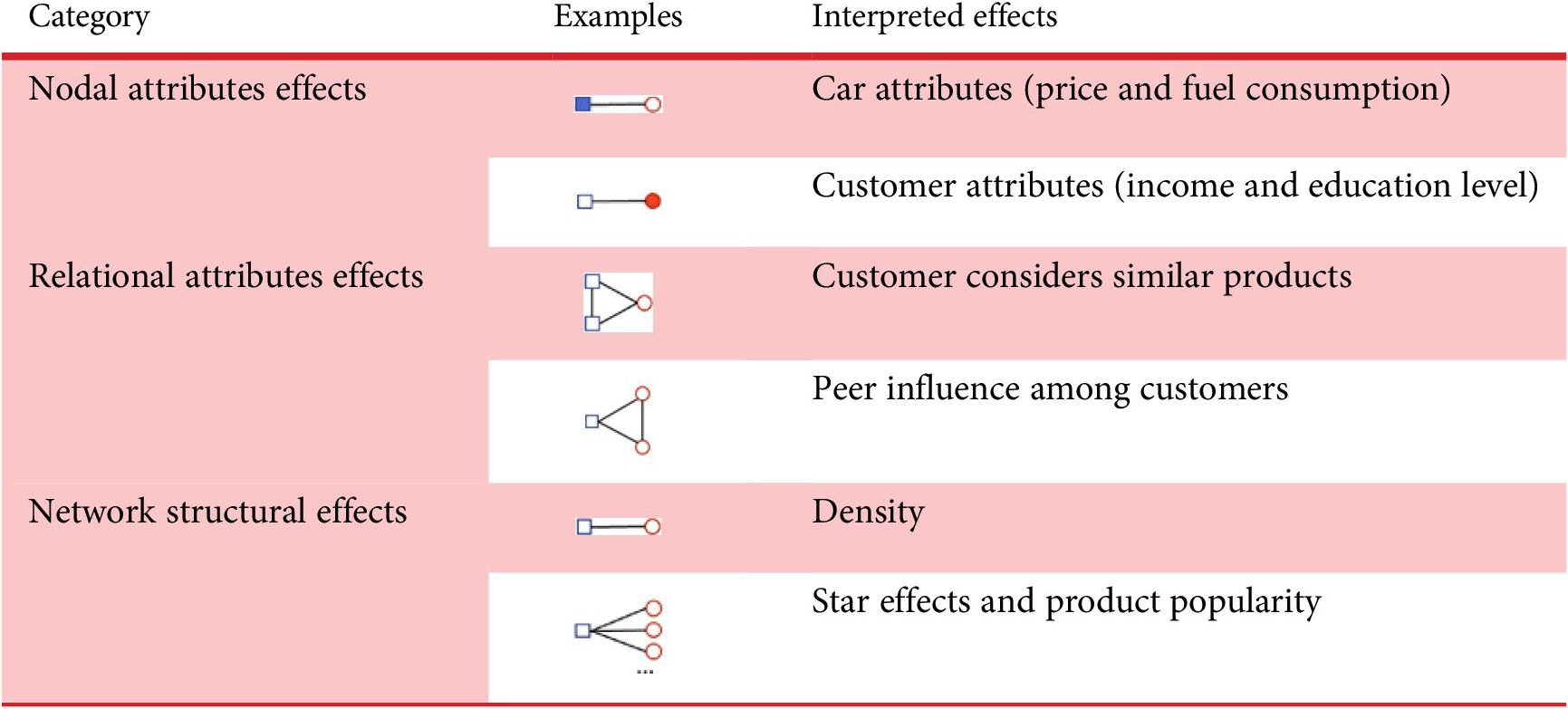
Note: The blue square represents the product, and the red circle represents the customer. The solid shape refers to the node of interest in modelling instead of the dyad relation.
3. Methodology
In this section, we first present a stepwise ERGM-based choice modelling approach (see Figure 2) that guides choice analysis, estimation, prediction and evaluation. The approach consists of five steps. In the first step, the revealed product choices are identified, and the choice set is defined along with the alternative-specific attributes obtained from a large-scale product database. Then, the customer–product bipartite networks are constructed and the choice scenarios are defined. Step 2 is about ERGM modelling that includes identifying critical network statistics and utilising additional settings and constraints (see Section 3.2) to ensure that the ERGM-based choice models accurately capture the given choice scenarios. Based on the models established in Step 2, Step 3 estimates the model parameters and compares the results of the models with different configurations (see Section 4.2). This step is critical because, by analysing similarity and differences, we build a knowledge base to understand consistency and interpretability of distinct ERGMs when applied to the same choice problem. In Step 4, the proposed ERGM-based choice prediction method is implemented. The mathematical procedure and the derivation are presented in Section 3.1. Step 5 is to select appropriate criteria to evaluate the predictive performance of the ERGM-based choice models. The criteria adopted in this study are based on two metrics: the Top-N probability (see Section 3.3.1) and the market share ranking (see Section 3.3.2). It should be noted that Steps 4 and 5 are essential to help draw valuable insights on the distinctions and connections between traditional utility-based and network-based approaches in choice modelling.

Figure 2. Overview of the exponential random graph model-based choice modelling research approach.
3.1 A new mathematical procedure for computing the predicted choice probability using ERGM
In this section, we propose a novel method for calculating the choice probability (i.e., the linking probability in the network context) based on ERGM. To predict the existence of a particular link, an important concept, called change statistics, must be introduced. Change statistics emerge when considering the probability of a single dyad having a link given the rest of the network. The vector of change statistics of a link is defined as follows (Hunter et al. Reference Hunter, Handcock, Butts, Goodreau and Morris2008):
where
![]() is the network
is the network $ \mathbf{y} $
with edge
$ \mathbf{y} $
with edge $ (i,j) $
added if absent (and unchanged if present), and
$ (i,j) $
added if absent (and unchanged if present), and $ {\mathbf{y}}_{\mathbf{ij}}^{-} $
is the network
$ {\mathbf{y}}_{\mathbf{ij}}^{-} $
is the network $ \mathbf{y} $
with edge
$ \mathbf{y} $
with edge $ (i,j) $
removed if present (and unchanged if absent). Then, based on Eq. (1), the probabilities of both networks
$ (i,j) $
removed if present (and unchanged if absent). Then, based on Eq. (1), the probabilities of both networks
![]() and
and $ {\mathbf{y}}_{\mathbf{ij}}^{-} $
can be expressed as follows:
$ {\mathbf{y}}_{\mathbf{ij}}^{-} $
can be expressed as follows:


By dividing those two formulas, we obtain

We can further write the formulas of conditional probabilities:

Given the fact that $ {\Pr}_{\boldsymbol{\unicode{x03B8}}; \mathbf{g}}({Y}_{ij}=1|{\mathbf{y}}^{\mathbf{c}})+{\Pr}_{\boldsymbol{\unicode{x03B8}}; \mathbf{g}}({Y}_{ij}=0|{\mathbf{y}}^{\mathbf{c}})=1 $
, we can rewrite the equation as follows:
$ {\Pr}_{\boldsymbol{\unicode{x03B8}}; \mathbf{g}}({Y}_{ij}=1|{\mathbf{y}}^{\mathbf{c}})+{\Pr}_{\boldsymbol{\unicode{x03B8}}; \mathbf{g}}({Y}_{ij}=0|{\mathbf{y}}^{\mathbf{c}})=1 $
, we can rewrite the equation as follows:
 $$ {\Pr}_{\boldsymbol{\unicode{x03B8}}; \mathbf{g}}({Y}_{ij}=1|{\mathbf{y}}^{\mathbf{c}})={\mathrm{logit}}^{-1}(\boldsymbol{\unicode{x03B8}} \cdot {\Delta}_{ij}\mathbf{g}(\mathbf{y})), $$
where $ {\mathbf{y}}^{\mathbf{c}} $
is the remaining network structure without the edge
$ {\mathbf{y}}^{\mathbf{c}} $
is the remaining network structure without the edge $ (i,j) $
, and
$ (i,j) $
, and $ {\Pr}_{\boldsymbol{\unicode{x03B8}}; \mathbf{g}}({Y}_{ij}=1|{\mathbf{y}}^{\mathbf{c}}) $
denotes how likely the link
$ {\Pr}_{\boldsymbol{\unicode{x03B8}}; \mathbf{g}}({Y}_{ij}=1|{\mathbf{y}}^{\mathbf{c}}) $
denotes how likely the link $ {Y}_{i,j} $
is to exist given the remaining network structure. Eq. (7) presents the mathematical foundation of the network link prediction (i.e., the choice prediction) based on the ERGM formula together with the change statistics.
$ {Y}_{i,j} $
is to exist given the remaining network structure. Eq. (7) presents the mathematical foundation of the network link prediction (i.e., the choice prediction) based on the ERGM formula together with the change statistics.
In the multinominal choice scenario, where each customer can have only one choice among multiple alternatives, the formula of link prediction in a bipartite customer–product network can be developed. Without loss of generality, we assume that each customer has three products (e.g., cars) in a choice set, and a customer $ n $
is allowed to make a single purchase decision among the three car models,
$ n $
is allowed to make a single purchase decision among the three car models, $ i $
,
$ i $
, $ j $
and
$ j $
and $ k $
(as illustrated in Figure 3).
$ k $
(as illustrated in Figure 3).
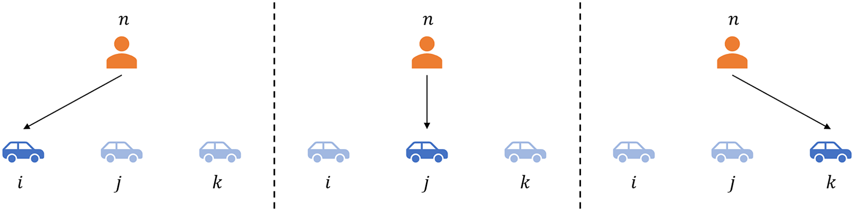
Figure 3. Illustration of the choice situation where a customer makes a choice among three alternatives. A customer $ n $
is allowed to make a purchase decision among the three car models, car
$ n $
is allowed to make a purchase decision among the three car models, car $ i $
, car
$ i $
, car $ j $
and car
$ j $
and car $ k $
. The figure illustrates the three choice scenarios.
$ k $
. The figure illustrates the three choice scenarios.
Based on the assumption that a customer chooses only one among the three alternatives, the following relation of the link probability holds:
 $$ {\displaystyle \begin{array}{l}{\Pr}_{\boldsymbol{\unicode{x03B8}}; \mathbf{g}}({Y}_{ni}=1,{Y}_{nj}=0,{Y}_{nk}=0|{\mathbf{y}}^{\mathbf{c}})+\\ {}{\Pr}_{\boldsymbol{\unicode{x03B8}}; \mathbf{g}}({Y}_{ni}=0,{Y}_{nj}=1,{Y}_{nk}=0|{\mathbf{y}}^{\mathbf{c}})+\\ {}{\Pr}_{\boldsymbol{\unicode{x03B8}}; \mathbf{g}}({Y}_{ni}=0,{Y}_{nj}=0,{Y}_{nk}=1|{\mathbf{y}}^{\mathbf{c}})=1,\end{array}} $$
where $ {Y}_{ni},{Y}_{nj},{Y}_{nk} $
denote the link between customer
$ {Y}_{ni},{Y}_{nj},{Y}_{nk} $
denote the link between customer $ n $
and each car model, respectively, and
$ n $
and each car model, respectively, and $ {\mathbf{y}}^{\mathbf{c}} $
denote the remaining network structure.
$ {\mathbf{y}}^{\mathbf{c}} $
denote the remaining network structure.
The conditional probability of link existence between node pairs $ \left(n,i\right) $
,
$ \left(n,i\right) $
, $ \left(n,j\right) $
and
$ \left(n,j\right) $
and $ \left(n,k\right) $
can be expressed as follows:
$ \left(n,k\right) $
can be expressed as follows:


Further, the marginal probability of numerators in Eqs. (9)–(11) can be represented by the ERGM in Eq. (1). Thus, we can rewrite Eqs. (9)–(11) as follows:


where
![]() denotes the network
denotes the network $ \mathbf{y} $
with link
$ \mathbf{y} $
with link $ {Y}_{n,i} $
present and links
$ {Y}_{n,i} $
present and links $ {Y}_{n,j} $
and
$ {Y}_{n,j} $
and $ {Y}_{n,k} $
absent,
$ {Y}_{n,k} $
absent,
![]() denotes the network
denotes the network $ \mathbf{y} $
with link
$ \mathbf{y} $
with link $ {Y}_{n,j} $
present and links
$ {Y}_{n,j} $
present and links $ {Y}_{n,i} $
and
$ {Y}_{n,i} $
and $ {Y}_{n,k} $
absent,
$ {Y}_{n,k} $
absent,
![]() denotes the network
denotes the network $ \mathbf{y} $
with link
$ \mathbf{y} $
with link $ {Y}_{n,k} $
present and links
$ {Y}_{n,k} $
present and links $ {Y}_{n,i} $
and
$ {Y}_{n,i} $
and $ {Y}_{n,j} $
absent.
$ {Y}_{n,j} $
absent.
By taking the division of Eqs. (12) and (13),

By taking the division of Eqs. (12) and (14),

Given a linear system of three equations of (8), (15) and (16), we can further solve for three unknown conditional probabilities as

This is exactly the probability that the link $ {Y}_{ni} $
exists given the rest of network structures, that is, the customer
$ {Y}_{ni} $
exists given the rest of network structures, that is, the customer $ n $
chooses car model
$ n $
chooses car model $ i $
given the rest of customer choices. Similarly, the probability that a customer chooses the other two products,
$ i $
given the rest of customer choices. Similarly, the probability that a customer chooses the other two products, $ j $
and
$ j $
and $ k $
, can be expressed in the following equations:
$ k $
, can be expressed in the following equations:


Eqs. (17)–(19) are the mathematical foundations of predicting customer choices based on the ERGM formula.
Based on the format of the probability distribution of link $ {Y}_{ni},{Y}_{nj},{Y}_{nk} $
, we note that if our network model only has exogenous effects (i.e., car attributes and customer attributes) as input to the model, the vector of the network statistic
$ {Y}_{ni},{Y}_{nj},{Y}_{nk} $
, we note that if our network model only has exogenous effects (i.e., car attributes and customer attributes) as input to the model, the vector of the network statistic $ \mathbf{g}(\mathbf{y}) $
will be a linear combination of only car attributes and customer attributes. Then, the probability distribution in Eqs. (17)–(19) will be equivalent to that of the ordinal multinomial logit (MNL) model (McFadden et al. Reference McFadden1973) under the assumptions aforementioned. In other words, when the ERGM only considers the nodal attributes but not the network statistics, the choice prediction using the ERGM can degenerate to an ordinary MNL model if certain model constraints are properly included. See the following subsection for details. However, if endogenous effects (i.e., network statistics) are considered, changes in network structure will have an impact on the predicted linking probability. In this case, the choice prediction based on ERGM will be different from that of DCM. In this study, we specifically investigated how the inclusion of network statistics in the choice prediction process influences the predictive accuracy of ERGM-based choice models.
$ \mathbf{g}(\mathbf{y}) $
will be a linear combination of only car attributes and customer attributes. Then, the probability distribution in Eqs. (17)–(19) will be equivalent to that of the ordinal multinomial logit (MNL) model (McFadden et al. Reference McFadden1973) under the assumptions aforementioned. In other words, when the ERGM only considers the nodal attributes but not the network statistics, the choice prediction using the ERGM can degenerate to an ordinary MNL model if certain model constraints are properly included. See the following subsection for details. However, if endogenous effects (i.e., network statistics) are considered, changes in network structure will have an impact on the predicted linking probability. In this case, the choice prediction based on ERGM will be different from that of DCM. In this study, we specifically investigated how the inclusion of network statistics in the choice prediction process influences the predictive accuracy of ERGM-based choice models.
3.2 ERGM settings and constraints
Traditional DCA is centred on decision analysis and makes model assumptions that chosen variables and choice sets remain stable throughout the modelling of a given decision scenario. These assumptions, however, do not hold in ERGM. For example, by default, there is no choice set defined in ERGM. The application of ERGM for different scenarios is often realised by means of different model configurations, that is, different combinations of edge and node settings and constraints. To enable the ERGM to model a general purchase decision scenario, two network statistics ( $ b2 factor $
(Morris et al. Reference Morris, Handcock and Hunter2008) and
$ b2 factor $
(Morris et al. Reference Morris, Handcock and Hunter2008) and $ b2\mathit{\operatorname{cov}} $
(Handcock & Hunter Reference Handcock and Hunter2018)) and two ERGM constraints (
$ b2\mathit{\operatorname{cov}} $
(Handcock & Hunter Reference Handcock and Hunter2018)) and two ERGM constraints ( $ offset $
(Hunter et al. Reference Hunter, Handcock, Butts, Goodreau and Morris2008) and
$ offset $
(Hunter et al. Reference Hunter, Handcock, Butts, Goodreau and Morris2008) and $ b1 degrees $
(Handcock & Hunter Reference Handcock and Hunter2018)) are adopted.
$ b1 degrees $
(Handcock & Hunter Reference Handcock and Hunter2018)) are adopted.
-
(i) $ b2\mathit{\operatorname{cov}} $
and
$ b2 factor $
: The main effect of a covariate and factor attribute effect for the second mode in a bipartite network (Handcock & Hunter Reference Handcock and Hunter2018). These two terms are used to carry quantitative and categorical nodal attributes corresponding to the product features that can influence customer preferences and then as input variables
$ \mathbf{g}(\mathbf{y}) $
for ERGM in Eq. (1).
$ b2\mathit{\operatorname{cov}} $
and
$ b2 factor $
: The main effect of a covariate and factor attribute effect for the second mode in a bipartite network (Handcock & Hunter Reference Handcock and Hunter2018). These two terms are used to carry quantitative and categorical nodal attributes corresponding to the product features that can influence customer preferences and then as input variables
$ \mathbf{g}(\mathbf{y}) $
for ERGM in Eq. (1). -
(ii)
$ offset $
: A vector of coefficients for the offset terms (Handcock & Hunter Reference Handcock and Hunter2018). In the customer–product bipartite network, this constraint is used to control how many product nodes are considered to form the links. This represents how many products can be linked to (i.e., considered by) each customer. Without this constraint, the default setting of ERGM will assume that each customer could link with all listed products. -
(iii)
$ constraints=b1 degrees $
: Together with the model terms in the formula and the reference measure, the constraints define the distribution of the networks being modelled (Handcock & Hunter Reference Handcock and Hunter2018). The constraint of
$ b1 degrees $
adopted in this study is used to limit the assumption that each customer node only links to one product node. This means that we assume that each customer can only make one choice from the choice set.


3.3 Evaluation criteria for prediction accuracy
Given that there is no established framework to evaluate ERGM predictions, we adopt two criteria that go beyond the evaluation of just the chosen alternative to consider the overall ranking. The first criterion evaluates the accuracy of the predicted customers’ Top-N choices, and the second one evaluates the predicted market share based on the predicted choice probability. These two criteria are introduced in the following two subsections.
Criterion 1: Top-N choice probability
Suppose that there are $ L $
customers and
$ L $
customers and $ M $
products, and every customer has a choice set, including
$ M $
products, and every customer has a choice set, including $ h $
products. The probability that the
$ h $
products. The probability that the $ {i}^{th} $
(
$ {i}^{th} $
( $ i=1,2,\dots, L $
) customer buys the
$ i=1,2,\dots, L $
) customer buys the $ {j}^{th} $
(
$ {j}^{th} $
( $ j=1,2,\dots, h $
) product is represented as
$ j=1,2,\dots, h $
) product is represented as $ {P}_{ij} $
. With the predicted choice probabilities of the top
$ {P}_{ij} $
. With the predicted choice probabilities of the top $ N $
(
$ N $
( $ N=1,2,\dots, h $
) alternatives in a choice set, we compare it against a customer’s final choice. If the predicted choice falls in the Top-N alternative set, then this is counted as one accurate prediction instance (Cremonesi, Koren & Turrin Reference Cremonesi, Koren and Turrin2010; Mottini et al. Reference Mottini, Lhéritier, Acuna-Agost and Zuluaga2018). For example, in the case of
$ N=1,2,\dots, h $
) alternatives in a choice set, we compare it against a customer’s final choice. If the predicted choice falls in the Top-N alternative set, then this is counted as one accurate prediction instance (Cremonesi, Koren & Turrin Reference Cremonesi, Koren and Turrin2010; Mottini et al. Reference Mottini, Lhéritier, Acuna-Agost and Zuluaga2018). For example, in the case of $ N=2 $
, if the actual choice is one of the two alternatives with the highest predicted probability, it is counted as a correct prediction. The advantage of the Top-N metric is that it does not only capture customers’ final choices (i.e., the Top 1 choice), but also evaluates the model’s performance in capturing a customer’s consideration behaviour. This metric provides a comprehensive evaluation of the model’s predictive power over the entire choice set. Based on this definition, the predictive accuracy can be defined as
$ N=2 $
, if the actual choice is one of the two alternatives with the highest predicted probability, it is counted as a correct prediction. The advantage of the Top-N metric is that it does not only capture customers’ final choices (i.e., the Top 1 choice), but also evaluates the model’s performance in capturing a customer’s consideration behaviour. This metric provides a comprehensive evaluation of the model’s predictive power over the entire choice set. Based on this definition, the predictive accuracy can be defined as
 $$ \hskip0.5em {Acc}_{topN}=\frac{L_{predict}}{L}, $$
where $ {L}_{predict} $
is the number of customers whose choices are correctly predicted to fall into the Top-N alternatives. With different configurations of the
$ {L}_{predict} $
is the number of customers whose choices are correctly predicted to fall into the Top-N alternatives. With different configurations of the $ N $
value, a trend curve can be obtained to delineate how the predictive accuracy would be influenced by the change of
$ N $
value, a trend curve can be obtained to delineate how the predictive accuracy would be influenced by the change of $ N $
.
$ N $
.
Criterion 2: market share ranking
While the Top-N choice probability criterion captures a choice model’s performance in predicting individual customers’ choices, the predictive power of models at the aggregate level, that is, the market level, is typically more relevant to enterprises. This approach reflects both the positioning and the specific market share of a product, thereby providing an indication of a product’s market competitiveness. The prediction-based market share can be divided into two steps. The first step is to predict the product that the $ {i}^{th} $
customer purchased based on the maximum choice probability in the choice set (
$ {i}^{th} $
customer purchased based on the maximum choice probability in the choice set ( $ \max {P}_{ij} $
,
$ \max {P}_{ij} $
, $ i=1,2,\dots, L;0\le j\le h $
). In the second step, we count the number of customers who purchase each unique product to derive each product’s market share reflecting all
$ i=1,2,\dots, L;0\le j\le h $
). In the second step, we count the number of customers who purchase each unique product to derive each product’s market share reflecting all $ L $
customers’ purchase behaviour.
$ L $
customers’ purchase behaviour.
After obtaining the predicted market shares of the products of interest, we can rank them based on their market shares and compare this ranking to the (real) reference market share. To quantify the predictive accuracy, two metrics are used. The first metric is focused on the ranking, and the Spearman’s rank correlation coefficient (Schober, Boer & Schwarte Reference Schober, Boer and Schwarte2018) is adopted to verify how well the rank of the most popular products (e.g., the top-K products ranked by the market share) predicted by the model matches the real data. The second metric compares the exact market share percentages, and computes the root mean square error (RMSE) (Chai & Draxler Reference Chai and Draxler2014) from comparing the predicted market shares to the actual one, and is calculated based on the following equation:
 $$ RMSE=\sqrt{\frac{1}{K}\sum \limits_{k=1}^K{\left( Real\_{MarketShare}_k- Predict\_{MarketShare}_k\right)}^2}. $$
There are several motivations for adopting these validation measures based on market share. First, the rank correlation coefficient of the market share reflects the models’ ability to forecast the popularity of the products in the overall market. Second, the RMSE value measures the accuracy of the market share predicted by the models compared to the actual market shares. Lastly, since both the market share ranking and its exact percentages are critical indicators to help enterprises assess a product’s market performance, the combination of the rank correlation coefficient and RMSE draws a more complete picture of the overall performance of the models.
4. Case study
4.1 Data preprocessing and scheme of test scenarios
Data source
The dataset used in this study is drawn from a large-scale revealed choice new car buyer survey conducted in the Chinese vehicle market in 2013. This dataset includes about 50,000 respondents and nearly 400 unique vehicle models. From this survey, various customer-related and car-related attributes are recorded, such as respondents’ gender and age, and vehicles’ price, power and brand. The database also records the stated consideration of vehicle models, in addition to the recorded final purchase. A more detailed summary of this dataset can be found in our previous paper (Sha et al. Reference Sha, Bi, Wang, Stathopoulos, Contractor, Fu and Chen2019). In line with our previous work, we narrow down the analysis to a single type of vehicle model. By focusing on the compact sedan standard vehicle segment, we seek to simplify the modelling and remove some sources of heterogeneity in decisions and choice sets. The analysis subset includes 18,054 compact sedan buyers, covering 84 unique compact sedan car models. Note that the stated considerations of alternatives are not limited to the compact sedan segment, although the final purchase was restricted to compact sedan purchases, making the total number of different car models covered in the analysis 281. Lastly, to improve the computational efficiency, 5000 customers are randomly sampled from the 18,054 compact sedan buyers to form the models’ training datasetFootnote 3. To test the sensitivity of results to the sampled data, we created three additional testing datasets of 5000 random customers (not overlapped with the training dataset) for analysis and prediction.
The treatment of choice sets
In this case study, two treatments of the choice set are considered. In the first treatment, we rely on stated information from customers to define a choice set of variable composition but identically sized (i.e., including the same number of alternatives). In the second treatment, it is assumed that each customer has the same fixed universal choice set consisting of all vehicle choice alternatives available on the market. Based on these assumptions, the two choice sets are defined as follows:
-
(i) ChoiceSet6: The first approach pursues behavioural realism by including stated consideration alternatives in a limited-size choice set. For every
$ N $
customer, we include information from the original survey data where they list between one to three ‘considered vehicle types’. While it is tempting to run models exclusively on this declared choice set, we note that the high degree of feature correlation inherent in enumerating close ‘runner-up’ options, leads to singularity and non-convergence issues in the DCA model. Therefore, we use insight from the literature (Hauser & Wernerfelt Reference Hauser and Wernerfelt1990) that customers typically consider three to six different car models in the buying process to build a more diverse choice set. In practice, we build a synthetic ChoiceSet6 where we append randomly selected car models from the complete set of 281 to each customer’s original stated consideration. -
(ii) ChoiceSetAll: The second approach is less behavioural but more comprehensive. We assume that the
$ N $
customers each have the same universal choice set consisting of 281 car models.


The scheme of model test
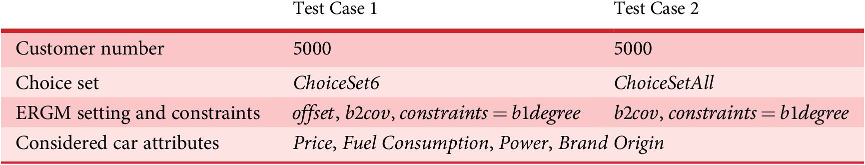
Based on the two choice set scenarios, ChoiceSet6 or ChoiceSetAll, our case study includes two test cases, as summarised in Table 3: Test Case 1 and Test Case 2. Because each customer can only make one choice in either choice scenario, $ constraints=b1 degrees $
needs to be applied in both test cases to constrain the number of links formed between a customer and his/her choice set to one. In addition, the
$ constraints=b1 degrees $
needs to be applied in both test cases to constrain the number of links formed between a customer and his/her choice set to one. In addition, the $ offset $
needs to be used in Test Case 1 to make sure the link is formed between the customer and his/her own choice set of six alternatives. Otherwise, the ERGM by default treats all available car nodes as being able to be connected.
$ offset $
needs to be used in Test Case 1 to make sure the link is formed between the customer and his/her own choice set of six alternatives. Otherwise, the ERGM by default treats all available car nodes as being able to be connected.
Table 3. The scheme of comparison
Abbreviation: ERGM, exponential random graph model base choice.
We select a few representative yet significant explanatory variables based on our prior work (Fu et al. Reference Fu, Sha, Huang, Wang, Fu and Chen2017). These explanatory vehicle attributes are: Price, Fuel Consumption, Power and Brand Origin. For all 281 car models in the 2013 Chinese market, the descriptive statistics of these four attributes are listed in Table 4. Additionally, given the large variation exhibited in each attribute and their skewed distributions, the log transformation (base 2) is applied to the price and engine power variables to offset the effect of large outliers, and z-score normalisation is applied to address the unit influence of those continuous variables.
Table 4. Descriptive statistics of the 281 sedan car attributes

4.2 ERGM estimation results
The estimated parameters of the ERGMs in the two cases are shown in Tables 5 and 6, respectively. Table 5 summarises the results of the ChoiceSet6 test case. For comparative purposes, we specify the same set of exogenous variables (i.e., car attributes) for all the ERGMs. Since the ERGM is uniquely positioned to handle endogenous factors (e.g., different network structures), we investigated two network effects, the degree effect and the star effect. The degree effect quantifies the influence of the number of a node’s connections on the formation of new links to that node. Hence, the degree effect reflects the popularity of a node. The star effect is a star-like structure with multiple edges connected to the central node. For example, 2-star represents the structure where there is one node connecting two links, that is, one vehicle model is purchased by two customers in our case. Please note that a specific star structure could be embedded. For example, for a node with three links, it has a degree of 3, three 2-stars and one 3-star. So, both effects capture the distribution of node-based edge counts and reflect the degree distribution information. However, the star effect could amplify the popularity of a node because the number of stars ( $ s $
) that could be obtained from a node with
$ s $
) that could be obtained from a node with $ n $
degrees is
$ n $
degrees is $ {C}_d^s $
. Please note that
$ {C}_d^s $
. Please note that $ {C}_d^s\ge d $
and the increase of one more degree will make the number of stars (n + 1) times greater. Therefore, there are four ERGMs to be tested.
$ {C}_d^s\ge d $
and the increase of one more degree will make the number of stars (n + 1) times greater. Therefore, there are four ERGMs to be tested. $ {ERGM}_{Null} $
only considers exogenous factors and does not include any network effects. Besides those exogenous factors, the
$ {ERGM}_{Null} $
only considers exogenous factors and does not include any network effects. Besides those exogenous factors, the $ {ERGM}_{Degree} $
model includes the network statistics of network degree (25+) and
$ {ERGM}_{Degree} $
model includes the network statistics of network degree (25+) and $ {ERGM}_{Star} $
includes the network statistics of network 2-star. Finally,
$ {ERGM}_{Star} $
includes the network statistics of network 2-star. Finally, $ {ERGM}_{Both} $
includes both network degree (25+) and network 2-star in the model.
$ {ERGM}_{Both} $
includes both network degree (25+) and network 2-star in the model.
Table 5. Estimated results of ChoiceSet6 test case with the comparison of different exponential random graph model base choices

Note: (1) The code *** indicates the 0.001 level of significance and ** indicates the 0.005 level of significance.
(2) Network degree (25+) represents the number of product nodes that have more than 25 connections to customer nodes.
(3) Network 2-star represents the number of star-like structure with two edges connected to the central products node.
Table 6. Estimated results of ChoiceSetAll test case with the comparison of different exponential random graph model base choices

Note: The code *** indicates the 0.001 level of significance.
Estimates for the ERGMs are shown in Table 5. When comparing the ERGMs including different network effects (i.e., $ {ERGM}_{Degree} $
,
$ {ERGM}_{Degree} $
, $ {ERGM}_{Star} $
and
$ {ERGM}_{Star} $
and $ {ERGM}_{Both} $
) to
$ {ERGM}_{Both} $
) to $ {ERGM}_{Null} $
, we note that the signs remain the same, whereas the magnitudes of the car attributes vary marginally. The changes are likely due to the correlation introduced by the newly added network structure variables. As for the estimated coefficients of the network structure, the negative sign of the network degree (25+)
Footnote
1 implies that in this particular sedan market, it is less likely for any specific car model to have more than 25 customers. The positive coefficient of network 2-star in ERGM indicates a higher probability of graphs with more 2-stars. Since more 2-stars come from nodes of a higher degree, the positive coefficient of this effect implies a higher degree of dispersion, so that there is a subset of car models that are highly popular among customers, compared with others. The running time of different models in R programming with Statnet package are reported based on an Intel i7-11700K CPU with a maximum frequency of 3.6 GHz.
$ {ERGM}_{Null} $
, we note that the signs remain the same, whereas the magnitudes of the car attributes vary marginally. The changes are likely due to the correlation introduced by the newly added network structure variables. As for the estimated coefficients of the network structure, the negative sign of the network degree (25+)
Footnote
1 implies that in this particular sedan market, it is less likely for any specific car model to have more than 25 customers. The positive coefficient of network 2-star in ERGM indicates a higher probability of graphs with more 2-stars. Since more 2-stars come from nodes of a higher degree, the positive coefficient of this effect implies a higher degree of dispersion, so that there is a subset of car models that are highly popular among customers, compared with others. The running time of different models in R programming with Statnet package are reported based on an Intel i7-11700K CPU with a maximum frequency of 3.6 GHz.
Table 6 shows the estimated results for the ChoiceSetAll test case. This corresponds to the choice situation where every customer considers all car models, which is equivalent to knowing the market-level information. In the $ {ERGM}_{Star} $
model, we have included network 2-star and network 3-star effects. The choice of the network statistics in Test Case 2 is different due to the features of the network under study as well as the convergence issues experienced with the ERGMs (Butts et al. Reference Butts, Morris, Krivitsky, Almquist, Handcock, Hunter, Goodreau and de Moll2014). For example, we found that the inclusion of network degree (25+) prevented ERGM convergence, and as a result, a different network structure, network 3-star, was adopted (see Section 6 for a detailed discussion on the model limitations). It is also observed that the magnitudes of the estimates changed primarily due to the inclusion of network effects. But, the signs of nodal variables are unaffected. This implies that while maintaining the same interpretation of the vehicle features in customer preferences, network effects are important in the formation of the consumer choice network. The predictive performance of these models will be evaluated in Section 4.3. The estimated positive 2-star and negative 3-star coefficients indicate some centralisation through high-degree nodes (i.e., popular cars are more likely to be purchased) but with a cap on the level of that centralisation indicated by the negative 3-star coefficient.
$ {ERGM}_{Star} $
model, we have included network 2-star and network 3-star effects. The choice of the network statistics in Test Case 2 is different due to the features of the network under study as well as the convergence issues experienced with the ERGMs (Butts et al. Reference Butts, Morris, Krivitsky, Almquist, Handcock, Hunter, Goodreau and de Moll2014). For example, we found that the inclusion of network degree (25+) prevented ERGM convergence, and as a result, a different network structure, network 3-star, was adopted (see Section 6 for a detailed discussion on the model limitations). It is also observed that the magnitudes of the estimates changed primarily due to the inclusion of network effects. But, the signs of nodal variables are unaffected. This implies that while maintaining the same interpretation of the vehicle features in customer preferences, network effects are important in the formation of the consumer choice network. The predictive performance of these models will be evaluated in Section 4.3. The estimated positive 2-star and negative 3-star coefficients indicate some centralisation through high-degree nodes (i.e., popular cars are more likely to be purchased) but with a cap on the level of that centralisation indicated by the negative 3-star coefficient.
On balance, the sign, significance and interpretation for most car attributes are consistent across the choice set treatments. Broadly, consumers are more likely to choose a car that is more affordable, powerful and with a European brand. In addition, network-based models can model features related to the market structure and thereby provide more information and opportunity for interpretation. Next, we further compare the structures based on predictive performance.
4.3 Evaluating the ERGM-based choice prediction
The probabilities of customer choices are calculated based on the method introduced in Section 3.1, from which we make the choice prediction. The Top-N choice probability and the market share ranking, corresponding to the individual choice prediction and market-level prediction, served as the two evaluation criteria for gauging the predictive power of all the models.
Test case 1: ChoiceSet6
Evaluating the Top-N choice probability. Figure 4 shows the average prediction accuracy with error bar of three different test datasets corresponding to the Top-N probability. In ChoiceSet6, N is set from 1 to 6. A higher Top-N accuracy indicates a better prediction of the overall trends of customers’ preferences over the entire consideration set, not merely for the final choice. For example, the average top 3 accuracy of the $ {ERGM}_{Null} $
model is 0.795, which indicates that the model correctly predicts 3975 customer (i.e., 79.5% of 5000) choices within the model’s top 3 predicted choices. We also calculated the area under the Top-N curve for each model in Figure 4 in order to assess the overall predictive performance. The baseline
$ {ERGM}_{Null} $
model is 0.795, which indicates that the model correctly predicts 3975 customer (i.e., 79.5% of 5000) choices within the model’s top 3 predicted choices. We also calculated the area under the Top-N curve for each model in Figure 4 in order to assess the overall predictive performance. The baseline $ {ERGM}_{Null} $
model yields an area under curve of 3.92, whereas the
$ {ERGM}_{Null} $
model yields an area under curve of 3.92, whereas the $ {ERGM}_{both} $
has the largest area under curve of 4.34, representing a 10.74% improvement over
$ {ERGM}_{both} $
has the largest area under curve of 4.34, representing a 10.74% improvement over $ {ERGM}_{Null} $
.
$ {ERGM}_{Null} $
.
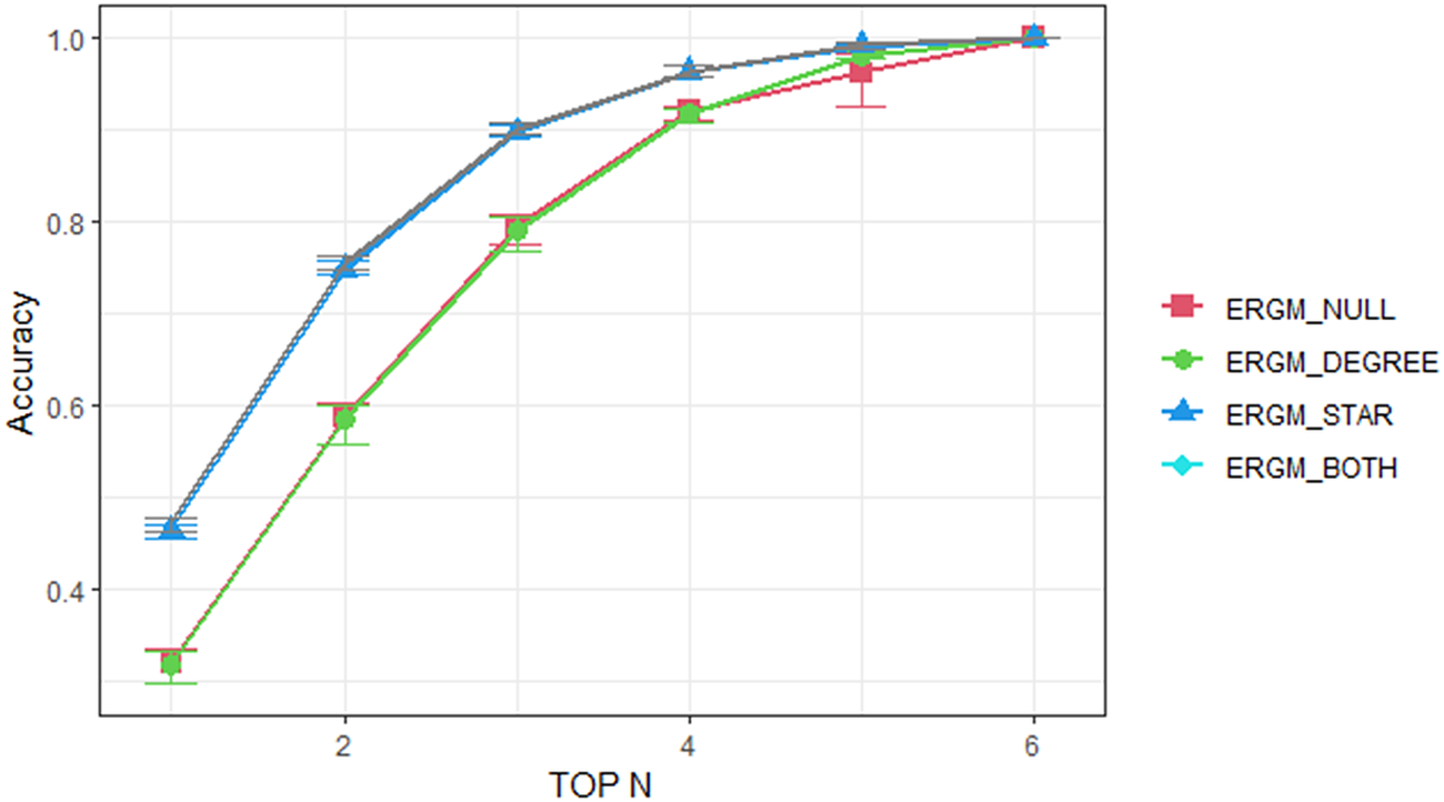
Figure 4. Top-N predictions results for three different test datasets (with mean and error bar) by different models in ChoiceSet6 test case.
The inclusion of network structures (i.e., the degree and star effects) in the ERGMs significantly enhances the model prediction, particularly the $ {ERGM}_{Star} $
and
$ {ERGM}_{Star} $
and $ {ERGM}_{Both} $
models in the top 1 and top 2 predictions. The findings indicate that more detailed network structures could capture latent information in customers’ purchase decisions, thereby leading to a better market forecast. As a broader insight, this result implies, in addition to vehicle attributes, that the embedded relations (e.g., competition or popularity) with other car models may also play an essential role in customers’ decision-making process. For example, the ‘star effect’ frequently occurs in the vehicle purchase network, so adding this structure helps explain the network formation process. The
$ {ERGM}_{Both} $
models in the top 1 and top 2 predictions. The findings indicate that more detailed network structures could capture latent information in customers’ purchase decisions, thereby leading to a better market forecast. As a broader insight, this result implies, in addition to vehicle attributes, that the embedded relations (e.g., competition or popularity) with other car models may also play an essential role in customers’ decision-making process. For example, the ‘star effect’ frequently occurs in the vehicle purchase network, so adding this structure helps explain the network formation process. The $ {ERGM}_{Degree} $
model does not produce significant improvement, indicating that the inclusion of the statistics of network degree (25+) is not as effective as the star effect in improving the model’s predictive performance.
$ {ERGM}_{Degree} $
model does not produce significant improvement, indicating that the inclusion of the statistics of network degree (25+) is not as effective as the star effect in improving the model’s predictive performance.
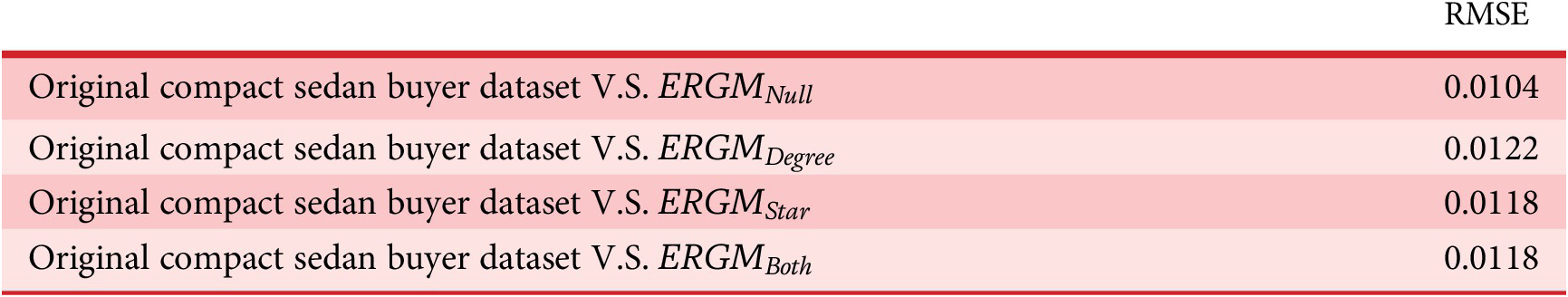
Evaluating the market share prediction. The predicted market share ranking of each car model is calculated, in which the predicted car model purchases are obtained from the predicted choice probabilities calculated by different ERGMs. Based on the predicted market share, the rank of each car model is obtained, and the resulting rank correlation and RMSEs are simply obtained by comparing it with the market share of the original compact sedan buyer dataset that covers all 84 unique car models. Figure 5 demonstrates the rank correlation coefficients from comparing the original sedan car buying dataset to each of the estimated models, and Table 7 shows the RMSE values.

Figure 5. Rank correlation comparison between different models and the baseline value from the original compact sedan buyer dataset.
Table 7. Root mean square errors (RMSEs) between the market share of the original compact sedan buyer dataset and the predicted market share of exponential random graph model base choices
In Figure 5, the rank correlation coefficient indicates to what extent the predicted popularity of the different models is consistent with that of the original compact sedan buyer dataset. A higher coefficient value means a better prediction of the market share ranking. It is observed that after introducing the 2-star network structure into the ERGM, an improvement of 0.15 in the rank correlation is achieved in both the $ {ERGM}_{Star} $
and
$ {ERGM}_{Star} $
and $ {ERGM}_{Both} $
models. However, we observe no significant improvement in the
$ {ERGM}_{Both} $
models. However, we observe no significant improvement in the $ {ERGM}_{Null} $
and
$ {ERGM}_{Null} $
and $ {ERGM}_{Degree} $
models. These results are in accordance with the ones observed from the Top-N prediction. Specifically, the inclusion of both network structures, that is, the star and degree effects, does not help to further improve the prediction. Instead, the ERGM with only star effect included performs the best among all models. This indicates that accounting for the broader network structures is not universally improving models, and that choosing suitable network structures is critical to constructing well-performing ERGMs. Based on our experience, an in-depth understanding of both the market context and the network structure is needed to help identify a list of potential network structure variables for initial comparison and testing.
$ {ERGM}_{Degree} $
models. These results are in accordance with the ones observed from the Top-N prediction. Specifically, the inclusion of both network structures, that is, the star and degree effects, does not help to further improve the prediction. Instead, the ERGM with only star effect included performs the best among all models. This indicates that accounting for the broader network structures is not universally improving models, and that choosing suitable network structures is critical to constructing well-performing ERGMs. Based on our experience, an in-depth understanding of both the market context and the network structure is needed to help identify a list of potential network structure variables for initial comparison and testing.
For the RMSE evaluation shown in Table 7, the smaller the RMSE value (the closer to zero), the better the prediction. All in all, the models achieve a decent prediction with RMSEs close to 0.01. No superiority of any ERGM is observed. This means that ERGMs, with the inclusion of specified network structures, perform better than $ {ERGM}_{Null} $
in predicting the overall market share ranking but achieves comparable, or slightly worse prediction for the market share percentages.
$ {ERGM}_{Null} $
in predicting the overall market share ranking but achieves comparable, or slightly worse prediction for the market share percentages.
Test case 2: ChoiceSetAll
In the ChoiceSetAll treatment,Footnote
2 every individual customer will have the same choice set that consists of the same number of alternatives, that is, 281 vehicles, from the entire (simulated) market. Figure 6 shows that $ {ERGM}_{Null} $
yields a better overall prediction accuracy with an area under curve of
$ {ERGM}_{Null} $
yields a better overall prediction accuracy with an area under curve of $ 214.30 $
, whereas
$ 214.30 $
, whereas $ {ERGM}_{Star} $
shows a lower accuracy measured by area under curve of
$ {ERGM}_{Star} $
shows a lower accuracy measured by area under curve of $ 180.37 $
. This implies that when modelling the scenario in which each customer faces all the car alternatives, adding the star-network effect does not help to improve the model performance. It could be the reason that in such a ChoiceSetAll scenario, each customer has already had access to the market-level information from the choice set. So, adding additional network structures does not further improve the predictive power of the model. This calls for caution when including network structures in the model for prediction purposes, as the types of network structures, the potential correlations between network effects and nodal attributes, the assumptions on choice scenarios, the size of choice set and the size of the test data could all influence the model performance. An evaluation of the model’s prediction accuracy benchmarked on the null model is always recommended before the final adoption of a model with network structures included.
$ 180.37 $
. This implies that when modelling the scenario in which each customer faces all the car alternatives, adding the star-network effect does not help to improve the model performance. It could be the reason that in such a ChoiceSetAll scenario, each customer has already had access to the market-level information from the choice set. So, adding additional network structures does not further improve the predictive power of the model. This calls for caution when including network structures in the model for prediction purposes, as the types of network structures, the potential correlations between network effects and nodal attributes, the assumptions on choice scenarios, the size of choice set and the size of the test data could all influence the model performance. An evaluation of the model’s prediction accuracy benchmarked on the null model is always recommended before the final adoption of a model with network structures included.

Figure 6. Top-N predictions results for three different test datasets (with mean and error bar) by different models in ChoiceSetAll test case.
5. Implications for engineering design
In this section, we present an improved DBD framework that integrates the ERGM-based choice model. The utility of the ERGM-based DBD framework is demonstrated in Section 5.2 by comparing the results of the MNL choice model (a traditional DCM commonly used in the DCA literature) with the ERGM-based choice model.
5.1. ERGM-based choice analysis for design
Based on the classic DBD framework (Chen et al. Reference Chen, Hoyle and Wassenaar2012), an improved DBD framework that integrates the ERGM-based choice model is proposed in Figure 7. In this framework, the grey boxes indicate the entities and events that belong to the original DBD framework. For example, the expected utility, in the ERGM-based framework, is still the key entity to merge the marketing and engineering domains into a single enterprise-driven decision-making framework. The coloured boxes indicate the place where the traditional discrete choice analysis is replaced by the ERGM-based choice analysis. As shown in the figure, the ERGM-based choice analysis considers not only the effect of product attributes on customer choices but can also the effect of network statistics g(y). These network statistics can be used to model the influence of social effects, product relations and any market effects that capture the interactions between customers and products on customers’ choice behaviour. With the inclusion of these network features, it is expected that a higher prediction accuracy of the choices and, therefore, the demand (Q) can be achieved. This hypothesis will be validated in the next section via a comparative study. The design implication of choice modelling is embodied through the successful prediction of market demand that can be used to construct the expected utility function (E(U)). From there, an optimisation problem can be formulated to find the optimal design options X and the price P that maximise E(U) subject to constraints, such as cost. Since the formulation of such a design problem has been extensively studied (Wassenaar & Chen Reference Wassenaar and Chen2003; Wang, Kannan & Azarm Reference Wang, Kannan and Azarm2011; Shin & Ferguson Reference Shin and Ferguson2017; Yip, Michalek & Whitefoot Reference Yip, Michalek and Whitefoot2019), we do not demonstrate it again in this paper. Instead, we will focus on validating the power of the ERGM-based choice model in predicting choices and demand, using the classical MNL choice model as the benchmark. It should be noted that, because of the introduction of network effects in this new DBD framework, it is now possible to test how different social relations, product associations and market effects would influence the design of product attribute.
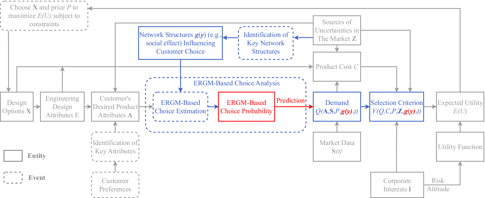
Figure 7. Decision-based design framework enhanced by network models. The grey boxes are the entities and events from the referred decision-based design framework; the coloured boxes belong to the proposed ERGM-based choice analysis.
5.2 Comparing the multinomial logit DCM and ERGM-based choice model
In this comparative study, we choose the commonly used MNL choice model as a representative DCM and use it as the baseline to compare against the model $ {ERGM}_{Both} $
. We compare their model estimates as well as their prediction accuracy of choices.
$ {ERGM}_{Both} $
. We compare their model estimates as well as their prediction accuracy of choices.
Comparing the model estimates
The estimated parameters of the DCM and $ {ERGM}_{Both} $
in ChoiceSet6 test case are shown in Table 8. For a fair comparison, we specify the same set of exogenous variables (i.e., car attributes) for both DCM and ERGM. The first observation is that the magnitudes of the estimates differ notably between the DCM and
$ {ERGM}_{Both} $
in ChoiceSet6 test case are shown in Table 8. For a fair comparison, we specify the same set of exogenous variables (i.e., car attributes) for both DCM and ERGM. The first observation is that the magnitudes of the estimates differ notably between the DCM and $ {ERGM}_{Both} $
. But, the signs of the estimates of these two models are mostly similar, except for fuel consumption. The sign coefficient for fuel consumption is expected to be negative, indicating that a car with lower fuel consumption is more desirable. The results show that the estimate of fuel consumption in
$ {ERGM}_{Both} $
. But, the signs of the estimates of these two models are mostly similar, except for fuel consumption. The sign coefficient for fuel consumption is expected to be negative, indicating that a car with lower fuel consumption is more desirable. The results show that the estimate of fuel consumption in $ {ERGM}_{Both} $
is more interpretable. The counter-intuitive coefficient of fuel consumption in the MNL model could be caused by the collinearity between input model terms (e.g., high fuel-consumption cars usually also have higher power). Also, we noticed that in the MNL model, car models with brands from Japan are more favourable than those from the United States, which is the opposite case in ERGM, where car models with brands from the United States are slightly more preferred. We argue that the interpretation of the ERGM model is more reasonable since it takes into account the overall network structure (i.e., market-level information).
$ {ERGM}_{Both} $
is more interpretable. The counter-intuitive coefficient of fuel consumption in the MNL model could be caused by the collinearity between input model terms (e.g., high fuel-consumption cars usually also have higher power). Also, we noticed that in the MNL model, car models with brands from Japan are more favourable than those from the United States, which is the opposite case in ERGM, where car models with brands from the United States are slightly more preferred. We argue that the interpretation of the ERGM model is more reasonable since it takes into account the overall network structure (i.e., market-level information).
Table 8. Estimated results of ChoiceSet6 test case with the comparison between $ {ERGM}_{Both} $
and DCM
$ {ERGM}_{Both} $
and DCM
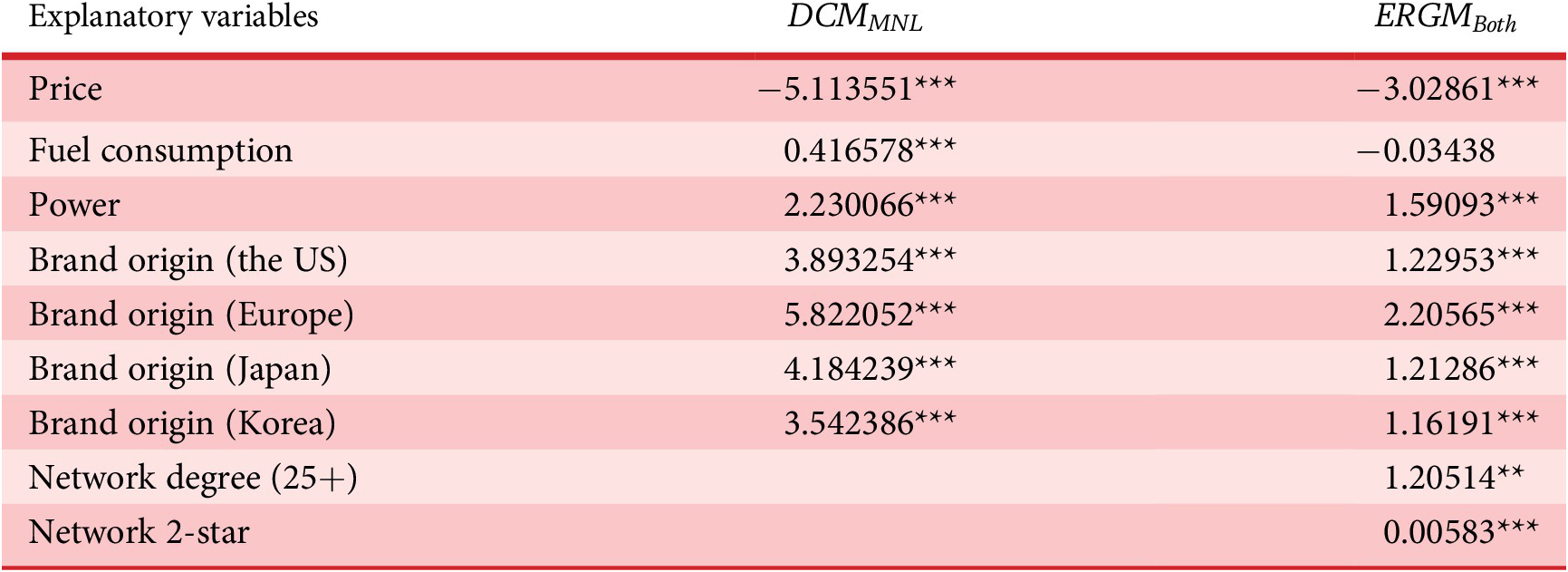
Note: The code *** indicates the 0.001 level of significance and ** indicates the 0.005 level of significance.
Comparing the predictive performance
Still taking ChoiceSet6 as an example, as shown in Figure 8, it is observed that the Top-N prediction accuracy of $ {ERGM}_{both} $
is higher than that of DCM, indicating that ERGM outperforms MNL when predicting the overall trends of customers’ preferences over the entire consideration set. Regarding the prediction of market share ranking, the rank correlation coefficient for
$ {ERGM}_{both} $
is higher than that of DCM, indicating that ERGM outperforms MNL when predicting the overall trends of customers’ preferences over the entire consideration set. Regarding the prediction of market share ranking, the rank correlation coefficient for $ {ERGM}_{both} $
is 0.76, which is higher than DCM (0.607), indicating the superiority of
$ {ERGM}_{both} $
is 0.76, which is higher than DCM (0.607), indicating the superiority of $ {ERGM}_{both} $
in predicting the popularity of products in the overall market. In terms of the prediction of market share percentages, both
$ {ERGM}_{both} $
in predicting the popularity of products in the overall market. In terms of the prediction of market share percentages, both $ {ERGM}_{both} $
(0.0118) and DCM (0.0104) achieve about equal prediction with RMSEs close to 0.01, but no superiority of
$ {ERGM}_{both} $
(0.0118) and DCM (0.0104) achieve about equal prediction with RMSEs close to 0.01, but no superiority of $ {ERGM}_{both} $
is observed.
$ {ERGM}_{both} $
is observed.

Figure 8. Top-N predictions for DCM and $ {ERGM}_{Both} $
model in ChoiceSet6 test case.
$ {ERGM}_{Both} $
model in ChoiceSet6 test case.
In short, the results reveal that, in addition to having better interpretability, ERGM with network structures ( $ {ERGM}_{both} $
) also outperforms DCM in predictive powers of both the individual choice behaviours and the overall market shares, measured by the Top-N choice prediction accuracy, rank correlation of the market share as well as the market percentage RMSE. This outperformance further validates the rationality of integrating ERGM analysis into DBD framework as shown in Figure 7.
$ {ERGM}_{both} $
) also outperforms DCM in predictive powers of both the individual choice behaviours and the overall market shares, measured by the Top-N choice prediction accuracy, rank correlation of the market share as well as the market percentage RMSE. This outperformance further validates the rationality of integrating ERGM analysis into DBD framework as shown in Figure 7.
5.3 Discussion on theoretical foundation of DCM and ERGM-based choice model
As stated in Section 1, the basic forms of DCMs have restrictions due to their assumptions on the independencies between alternatives and the rationality of customers, and the network-based approach addresses these limitations by treating the choice prediction as a link prediction problem so that specific network models, that is, ERGM in this study, can help relax those assumptions. This is because in contrast to the usual general linear model, which assumes that customers’ considerations are independent (Figure 9a), network models assume that the formation of links is dependent on other links in the network. For example, the link formed between Customer 1 and Product A may be because Customers 1 and 2 both considered Product B, and meanwhile Customer 2 also considered Product A (the case shown in Figure 9b), or may be because both Customers 2 and 3 considered Product A (the case shown in Figure 9c). In ERGM, different network configurations, such as the ‘shared-partner’ structures (e.g., cars being considered by common customers), as shown in Figure 9b, and ‘star effects’ (e.g., the cars being considered by many customers), as shown in Figure 9c, can model those interdependent effects.
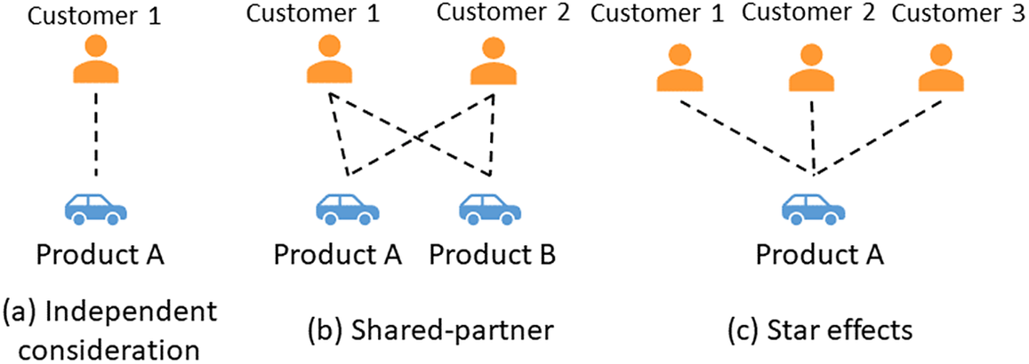
Figure 9. The interdependency assumption underlying the network-based models.
The differences between the two models’ estimates and outperformed prediction ability of ERGM are primarily caused by the distinction between the calculation of choice probabilities in DCM and ERGM and their resulting maximum likelihood estimation processes. In DCM, the choice probability is calculated within the given choice set. However, in ERGM, the calculation takes into account the entire network structure because of the inclusion of network statistics. This sheds light on the interpretation of the decision-making assumptions underlying the two models. In DCM, the model estimation assumes that each customer evaluates their own choice set and makes a final choice by picking the alternative with the maximum utility. That is, any comparison of utilities is done within the choice set, and customers do not refer to the alternatives outside that set. However, in ERGM, the linking probability between two nodes is calculated based on the information from the entire network, that is, the market. So, ERGM assumes that customers are aware of market-level information and while they are making a choice decision, such information will consciously or unconsciously affect their choice behaviours. This is what Shocker et al. (Reference Shocker, Ben-Akiva, Boccara and Nedungadi1991) mentioned the awareness set, which can provide additional cue information in memory to customers when they make decisions. Arguably, the configurations in network models represent a more realistic decision process where consumers are likely to be aware of all the car models in the entire set, and ERGMs can provide an avenue to examine that awareness effect on choice while also improving their own predictive abilities.
6. Conclusion
In this paper, we develop a novel ERGM-based choice prediction approach with the ability to compute individual choice probabilities in a given choice set. This approach, on the one hand, explore the customer choice prediction power of ERGM in a bipartite network setting, that is, the incorporation of network structures to improve the choice prediction accuracy. On the other hand, this approach is a key bridge between ERGM-based choice analysis and the concept of ‘utility’ in traditional DCMs when extending the classic DBD framework (Chen et al. Reference Chen, Hoyle and Wassenaar2012) to the DBD framework enhanced by network models. The utility of this approach is validated by using a vehicle market system as a case study. According to the results, we observe that the inclusion of network structures in ERGM yields a significant improvement in predicting individual choices as quantified by the Top-N choice prediction as well as the market share rank correlation validation. An important caveat to note for each model structure is that the predictive performance of ERGM is related to the selection of specific network structures. Therefore, an in-depth understanding of the market structure (i.e., network formation) will be key to identifying the set of most suitable and effective network structures for ERGM modelling. Relatedly, this choice will likely vary with the decision context and sample analysed.
Based on this study, our future work unfolds in two directions. First, a multidimensional choice network is under investigation, where more complex relations at each layer of nodes, for example, product associations at the product node layer and social interactions at the customer layer, are allowed, so that it provides a framework for researchers to study how the interdependencies of multiple layers of nodes can influence customers’ choice behaviours, and thus helps to forecast the market share. Second, the authors see the need of developing a feature engineering approach for automatic network structure identification and selection in support of constructing ERGMs with network structural effects.
Financial support
The authors acknowledge the financial support from NSF-CMMI-2005661 and 2203080, the Ford-Northwestern Alliance Project and the Vice Chancellor for Research and Innovation Seed Grant from the University of Arkansas. Partial financial support was provided to Stathopoulos from NSF-CAREER-1847537.
Appendix. Validating the representativeness of the training datasets
To check if the market share of the sampled training dataset (i.e., the dataset consists of 5000 car buyers) effectively represents the market share of the compact sedan in the original compact sedan buyer dataset (i.e., the dataset including all 18,054 car buyers), the market shares from both datasets are compared. After obtaining and ranking the market share of every compact sedan from the original dataset, the top 10 most popular compact sedan car models are identified (see the blue bars in Figure A1). In the same figure, the orange bars represent the market share and the ranks of those top 10 car models obtained from the training dataset.

Figure A1. Market share comparison of the original compact sedan purchased dataset and the training dataset.
As shown in Figure A1, the rank of the market share of the top 10 compact sedans from the training dataset has a high rank correlation (0.96) with the original data, indicating that the training dataset is a good representation of the original compact sedan buyer dataset. This conclusion is confirmed by the low RMSE value of 0.002. To further evaluate the market share correlation and variation between the training dataset and the original compact sedan buyer dataset, the rank correlation and market share RMSE of the total set of 84 unique compact sedan car models are calculated. The results are 0.94 and 0.0027, respectively. Therefore, the representativeness of the training datasets is confirmed.


 Open access