


1. Introduction
Sparse reconstruction is a technique used to obtain accurate details about the full scale features of a system using a sparse subset of information (e.g., a few pixels or measurements within the system) and has been the subject of interest for some decades (Candès, Reference Candès2006; Donoho, Reference Donoho2006). Applications for such state estimation problems range from reconstructing faces from limited or corrupted data (Wright et al., Reference Wright, Yang, Ganesh, Sastry and Ma2008) to deblurring and improving image resolution (Dong et al., Reference Dong, Zhang, Shi and Wu2011) to estimating global sea surface temperatures (Manohar et al., Reference Manohar, Brunton, Kutz and Brunton2018; Callaham et al., Reference Callaham, Maeda and Brunton2019). The literature concerning state estimation and sparse reconstruction is rapidly developing. In the following, we motivate and present a brief review of the literature as it relates to the present study. For a more comprehensive review, we refer the interested reader to Manohar et al. (Reference Manohar, Brunton, Kutz and Brunton2018) and Nair and Goza (Reference Nair and Goza2019).
In general, the requirements for accurate sparse reconstructions from limited data are that (a) the basis underlying the data exhibits sparsity (as will be discussed) and (b) that full-state information for the system can be obtained or approximated a priori to generate a global basis applicable to any sample or instant (Brunton and Kutz, Reference Brunton and Kutz2019). For example, suppose a set of images of weathered ancient hieroglyphics are only partially discernible. If a library of images of known undamaged hieroglyphics is tabulated a priori, the principle of sparsity can be used to estimate the weathered hieroglyphics before they were damaged (Roman-Rangel et al., Reference Roman-Rangel, Odobez and Gatica-Perez2012). Further examples of sparse reconstruction exist over a diverse range of engineering disciplines. Liu et al. (Reference Liu, Zhang and Xu2017) demonstrated the use of sparsity to monitor and detect faults in an industrial Tennessee Eastman Process using a novel variation of principle component analysis. Bao et al. (Reference Bao, Shi, Wang and Li2017) showed the use of sparse strain sensors to estimate the full stress state of a structure using a Fourier basis. Iyer et al. (Reference Iyer, An and Subramanian2020) used recurrent neural networks (NNs) and sparse observations for reconstructing and forecasting road traffic.
Sparse reconstruction may also be extended to data-assimilation applications. Brajard et al. (Reference Brajard, Carassi, Bocquet and Bertino2020) demonstrated assimilating data from noisy sparse observations for predicting a chaotic 40-variables Lorenz system using a convolutional NN. Further applications of data-assimilation using sparsity remain to be explored. For example, if the entire flow field in the neighborhood of a gas turbine blade is simulated and a global basis tabulated, the flow field in the neighborhood of a real turbine blade fitted with flow sensors can be estimated. Such a reconstruction technique is widely applicable to any system exhibiting many degrees of freedom. Therefore, the number of possible applications for sparse reconstructions in science and engineering is large.
There remains much to be done in order to test the limitations of sparse reconstructions numerically, experimentally, and via data-assimilation for a variety of engineering systems. For example: how do variations of nondimensional parameters that characterize a system impact the reconstruction? How many known full-state snapshots are required to generate a global basis? How many sparse sensors or probes are needed to achieve a desired reconstruction accuracy? Where should the probes be placed? These are some of the underlying questions that motivate the current study seeking to expand the application of sparse sensing to engineering problems.
The key underlying principle that allows for full reconstructions using only limited measurements is the sparsity of the representative basis. For the application of interest, a suitable basis must be chosen onto which to project the sparse signal (the limited measurements) for the full reconstruction. The basis of choice depends on the data in question but is typically taken to be either a Fourier transform (Candès and Wakin, Reference Candès and Wakin2008) or a data-driven basis such as the proper orthogonal decomposition (POD; Sirovich, Reference Sirovich1987; Berkooz et al., Reference Berkooz, Holmes and Lumley1993). If the basis contains many entries that are small (near-zero) then the system is said to exhibit sparsity. For example, a Fourier transform may indicate only a few frequencies have significant amplitudes. Sparse reconstruction takes advantage of the sparsity of the basis functions to produce full reconstructions (Brunton and Kutz, Reference Brunton and Kutz2019) that can yield surprisingly accurate full state estimations. For example, using POD as a representative basis Manohar et al. (Reference Manohar, Brunton, Kutz and Brunton2018) showed that using only seven probes they could reconstruct the full vorticity field of laminar flow over a cylinder exceeding 90% accuracy.
POD is a data-driven method commonly used as a basis for reconstructions due to its attractive properties of being energy optimal and having time-independent spatial modes, though other choices are possible (Bai et al., Reference Bai, Wimalajeewa, Berger, Wang, Glauser and Varshney2015; Jayaraman et al., Reference Jayaraman, Al Mamun and Lu2019). Manohar et al. (Reference Manohar, Brunton, Kutz and Brunton2018) demonstrated that the reconstruction accuracy is significantly improved if the choice of probe locations is made carefully such that it takes better advantage of the sparse basis. They demonstrated that the use of greedy algorithms to intelligently place probes within the flow improved the reconstructions greatly compared to random probe placement. However, this also depends on the complexity of the underlying system. When the analysis was applied to sea surface temperatures whose POD basis requires many more modes, the reconstruction accuracy relied more heavily on the optimal probe placement; pointing to the difficulty of reconstructing systems with a large range of spatio-temporal scales.
Several alternative methods originating in the fluid mechanics literature have been proposed for sensing turbulent flow structures and obtaining reconstructions, such as linear stochastic estimation (LSE; Adrian and Moin, Reference Adrian and Moin1988). In LSE, the state of the flow field is tabulated and conditioned upon the state of an event, leading to a linear map through an  $ {l}_2 $ minimization procedure. Several studies have demonstrated the fidelity of reconstructions based on the concept of LSE (Picard and Delville, Reference Picard and Delville2000; Lasagna et al., Reference Lasagna, Orazi and Iuso2013). Borée (Reference Borée2003) showed that LSE is equivalent to the so-called extended POD, where the temporal POD modes of one quantity are projected onto by the state of the flow field. This produces a set of extended modes revealing the spatial structures of the flow that are correlated with the quantity of interest. The extended POD framework is a straightforward and flexible approach offering alternative means of obtaining reconstructions using the temporal modes of the sparse information, as demonstrated by Hosseini et al. (Reference Hosseini, Martinuzzi and Noack2015). Extended POD was pushed further by Discetti et al. (Reference Discetti, Raiola and Ianiro2018) to obtain up-sampled time-resolved velocity fields from sparse sensors; demonstrating the flexibility of the framework.
Although the aforementioned techniques produce sparse reconstructions that are obtained entirely linearly, supervised machine learning provides a nonlinear framework with additional flexibility. In fact, POD itself is a form of unsupervised machine learning (Brunton et al., Reference Brunton, Noack and Koumoutsakos2020) and one may interpret the POD as an unsupervised NN with a single layer and linear activation function (Milano and Koumoutsakos, Reference Milano and Koumoutsakos2002). The use of NNs to obtain sparse reconstructions has seen recent attention in the literature. Nair and Goza (Reference Nair and Goza2019) demonstrated the ability of NNs to outperform the linear counterparts using a network of three layers for low Reynolds number flow over a flat plate at high angles of attack. Similarly, Erichson et al. (Reference Erichson, Mathelin, Yao, Brunton, Mahoney and Kutz2019) introduced a “shallow” neural network (SNN) consisting of two layers for reconstructing laminar flow over a cylinder with high fidelity. They further applied this method to a comparatively more challenging numerical simulation of isotropic turbulence and found difficulty in predicting future states. They discussed the use of regularization of the loss function to avoid overfitting; a problem that can easily arise with limited training data. Intelligent choices for loss functions offers promising potential for improved NN performance and generalization. For example, imposing physical constraints on the loss function has been demonstrated as a successful approach for a variety of systems governed by partial differential equations (Raissi et al., Reference Raissi, Perdikaris and Karniadakis2019; Sun and Wang, Reference Sun and Wang2020). More recently, convolutional NNs have been demonstrated for flow reconstruction from wall shear measurements in a turbulent channel flow (Guastoni et al., Reference Guastoni, Güemes, Ianiro, Discetti, Schlatter, Azizpour and Vinuesa2020), however, the inherent spatial dependence renders convolution-based approaches unattractive for the particular case of spatially sparse reconstruction. This does however represent progress in the direction of reconstructing turbulent flows, as their inherent range of spatial and temporal scales makes them significantly more challenging than the laminar case.
The present study focuses on the problem of sparse sensing motivated by the need to detect flow structures in aerospace applications. For example: to detect anomalous structures, the onset of stall over an aerofoil, or to inform control systems designed to reduce drag. Here, the focus is on the situation of an aerofoil in stalled conditions. We seek to explore how a global basis may be used to predict the unseen flow about a stalled aerofoil using limited single-point sensors placed in the flow.
As of yet, data-driven sparse sensing has not been widely applied to advective turbulent flows such as the case of a stalled aerofoil due to the inherently large range of scales and difficulty in capturing a low-order representation of the dynamics. As a result, the flow requires many modes compared to, for example, the case of a laminar cylinder (Figure 1) to capture the dynamics. This fact motivates exploration of reconstructions obtained outside the classic compressed sensing approach, which relies more heavily on optimal placement for systems with many modes. The present study seeks to explore how effectively the various linear and nonlinear approaches for sparse reconstruction perform for (a) a situation which is highly turbulent and (b) data generated via experiment and therefore contaminated by experimental noise.

Figure 1. Instantaneous velocity fields (a and b) from the particle image velocimetry (PIV) data (every fifth vector shown for clarity) presented in this study at two separate instants; highlighting the variation in the size of the separated wake. The singular values are shown in (c) normalized by the first singular value (inset: up to 9,000 modes). This is also shown for the laminar cylinder wake (dashed) of diameter  $ D $ at $ {Re}_D=100 $ from the Direct Numerical Simulation (DNS) of Brunton and Kutz (Reference Brunton and Kutz2019) for comparison.
The present study will be structured as follows. The experiments performed to obtain the two-dimensional time-resolved flow fields of the separated aerofoil are outlined in Section 2. The methodology used to select probe placements and obtain the sparse reconstructions with and without NN refinement is presented in Section 3. The results are presented in Section 4. Conclusions and outlook for future work are finally presented in Section 5.
2. Experimental Method
Particle image velocimetry (PIV) has seen widespread use in experimental fluid mechanics over the past decades due to its ability to obtain highly spatially-resolved instantaneous planar two-component velocity fields (Adrian et al., Reference Adrian, Adrian and Westerweel2011). Combined with time-resolved capabilities of high-speed cameras, it is the measurement method of choice for the present data-driven analysis due to the ability to generate large spatial domains (and resulting spatial modes) as well as time information at each point in the flow; enabling the sparse reconstruction investigation via a pseudo-probe analysis. The details of the data collection and postprocessing are outlined in the following sections.
2.1. Water flume experiment
To obtain planar time-resolved velocity fields on the suction side of a separated NACA 0012 aerofoil, a PIV campaign was performed in the water flume flow facility located at the University of Southampton as illustrated in Figure 2. A NACA 0012 aerofoil model of chord length  $ c=15 $ cm and span $ s=70 $ cm was fixed vertically in the center of the span of the flume immediately following the contraction into the test section. The aerofoil was fixed at angle of attack $ \alpha ={12}^{\circ } $ using a stepper motor attached to an overhead carriage system with precise control over the stepper motor angle. A four Megapixel Phantom v641 camera Vision Research Inc. Bus. Unit of AMETEKPhantom Digital High-Speed Cameras https://www.photonics.com/Products/Phantom_v641_Digital_High-Speed_Camera/pr46264 mounting a 105 mm Ex Sigma lens ( $ f=5.6 $) was directed upward from underneath the flume at a standoff distance 88 cm, resulting in a stream-wise wall-parallel field of view approximately 16 cm in the stream-wise direction $ x $ and 10 cm in the stream-normal wall-parallel direction $ y $. The field of view was illuminated via a set of sheet-forming optics directing laser light from a Litron 527 nm Nd:YLF high-speed laser into the test section from the side of the facility at a wall-normal height of $ {h}_L=248 $ mm from the bottom of the flume. The flume was filled until the water reached a height $ {h}_w=500 $ mm for which the maximum frequency of the flume pumps yielded a free stream velocity $ {U}_{\infty }=0.5 $ m/s corresponding to a Reynolds number based on the chord length $ {Re}_c=\frac{U_{\infty }c}{\nu }=\mathrm{75,000} $, where $ \nu $ is the kinematic viscosity.

Figure 2. Illustration of the experimental setup focusing on the test section of the water flume flow facility at the University of Southampton. The NACA 0012 aerofoil is illuminated from both sides, however, for this study, a field of view focusing on the suction side of the aerofoil is used to capture the separation of the wake. The water level  $ {h}_w $ and laser sheet level $ {h}_L $ are indicated.
To collect the images, Davis 8.3.1 PIV software was used with a LaVision high-speed controller to ensure synchronous timing of laser and camera. The flow was seeded with Vestosint 2157 polyamide particles of nominal diameter 55 μm verified to behave as faithful flow tracers. The seeding density was iteratively adjusted until a satisfactory number of particle reflections across the field of view were observed. The images were captured at full resolution (2560 × 1600 pixels) at a frequency of 750 Hz. In total, 9,000 separate snapshots were collected for data training purposes and one fully time-resolved run corresponding to 5,468 sequential snapshots across 7.3 seconds of continuous measurement was collected to test sparse reconstruction methodologies. At an angle of attack  $ \alpha ={12}^{\circ } $, substantial separation from the surface of the aerofoil was observed (Figure 1).
2.2. Data postprocessing
The images were background-subtracted and low frequency noise was attenuated using a convolution with a Gaussian high-pass filter of standard deviation of five pixels. A mask corresponding to the location of the aerofoil in the images was stored and applied during PIV processing. The images were processed using a verified in-house PIV code based in MATLAB with iterative interrogation window stepping from 64 × 64 pixels to 32 × 32 pixels to 24 × 24 pixels with 50% overlap. Subpixel displacements were obtained via a Gaussian 3-point fit, and detected outliers were flagged and replaced via local interpolation. Interrogation windows found to overlap with the image mask by greater than 25% were discarded.
For each component of the velocity field, the velocity was decomposed into a mean and fluctuating component  $ u=U+{u}^{\prime } $ and $ v=V+{v}^{\prime } $, where the capitals here denote the mean velocity field and the prime denotes the fluctuating components of the horizontal (stream-wise) $ u $ and vertical (stream normal) fields $ v $. To reduce the random noise of the PIV fields, the filtering method based on POD described in Raiola et al. (Reference Raiola, Discetti and Ianiro2015) was used (see Section 3.1) with the suggested value of the parameter $ F=0.999 $ (the ratio of forward to backward residuals of the rank-restricted POD reconstruction). The location of the rank-order filtering truncation (see Section 3.1) was found to correspond to only 5% of the energy of the velocity fluctuations. To improve the accuracy of the velocity fields, particularly in the separated region, gappy POD was employed using iterative replacement of detected outliers (Gunes et al., Reference Gunes, Sirisup and Karniadakis2006) until satisfactory convergence was achieved. It was verified that the number of POD modes used to reduce random noise and improve the accuracy of the velocity fields was greater than the number of modes used to test the sparse reconstructions.
3. Sparse Reconstruction Methodology
3.1. Proper orthogonal decomposition
For the present study, the POD (Sirovich, Reference Sirovich1987; Berkooz et al., Reference Berkooz, Holmes and Lumley1993) is used as a basis for the reconstruction due to its unique property as an energy-optimal basis. POD is commonly utilized as a basis for sparse reconstruction (Candès, Reference Candès2006), though other choices (such as a Fourier basis) are possible (Jayaraman et al., Reference Jayaraman, Al Mamun and Lu2019). In the present notation, the fluctuating velocity fields are rearranged into a matrix  $ \mathrm{U} $ of size $ {n}_t\times 2{n}_x $, where $ {n}_t $ is the number of snapshots and $ {n}_x $ is the total number of spatial points (PIV vectors). At each instant, the fluctuating horizontal velocity field $ {u}^{\prime } $ is appended row-wise with the vertical $ {v}^{\prime } $ resulting in twice the number of spatial points in the rows of $ \mathrm{U} $ (see e.g., Taira et al., Reference Taira, Brunton, Dawson, Rowley, Colonius, McKeon, Schmidt, Gordeyev, Theofilis and Ukeiley2017). Henceforth, capital $ U $ will denote the appended fluctuating velocity fields (not to be confused with the mean velocity fields). The POD is then calculated as:
 $$ \boldsymbol{U}=\boldsymbol{\Psi} \boldsymbol{\Sigma} \boldsymbol{\Phi}, $$
where  $ \boldsymbol{\Psi} $ is an orthogonal matrix of temporal modes of size $ {n}_t\times {n}_t $ satisfying $ {\boldsymbol{\Psi}}^T\boldsymbol{\Psi} =\mathrm{I} $ with corresponding columns $ {\boldsymbol{\psi}}_k $ containing the $ k $th temporal mode. $ \boldsymbol{\Sigma} $ is a diagonal matrix of singular values (the square root of the eigenvalues of the velocity autocorrelation) of size $ {n}_t\times {n}_t $ containing the relative contribution of each mode where $ {\sigma}_k $ is the $ k $th diagonal entry. Finally, $ \boldsymbol{\Phi} $ is an orthogonal matrix of spatial modes of size $ {n}_t\times 2{n}_x $ satisfying $ {\boldsymbol{\Phi}}^T\boldsymbol{\Phi} =\boldsymbol{I} $ with corresponding rows $ {\boldsymbol{\phi}}_k $ containing the $ k $th spatial mode. POD is an exact decomposition of the velocity fields, however, a low-order representation of the fields is easily obtained by imposing a rank-order truncation for $ k $ desired modes. POD is a data-driven decomposition in the sense that the number of available modes depends on the number snapshots used to perform the POD. Often in the literature, the temporal modes and the singular values are combined into a single matrix $ \boldsymbol{A}=\boldsymbol{\Psi} \boldsymbol{\Sigma} $ referred to as the POD coefficients with columns $ {\mathrm{a}}_k $ corresponding to the $ k $th mode coefficients across all samples and $ a{(t)}_k $ the kth mode coefficient for a particular sample at time $ t $. A truncated reconstruction corresponding to $ k $ modes is then obtained using the coefficients at a particular instant as
 $$ \boldsymbol{U}(t)=\sum \limits_1^ka{(t)}_k{\boldsymbol{\phi}}_k, $$
where, here, the explicit time dependence in  $ \boldsymbol{U}(t) $ is retained to emphasize it is a vector of fluctuating velocities of length $ 2{n}_x $ at time instant $ t $. A key feature of POD that allows for sparse reconstruction is in the time independence of the spatial modes $ {\boldsymbol{\phi}}_k $. With enough samples, the most energetic modes (associated to the underlying physical mechanisms) converge (i.e., the modes do not change with additional samples). For these time-independent energetic modes, the reconstruction becomes a matter of approximating $ A $ using a limited number of sensors. In practice, approximating the coefficients can be achieved in several ways including the use of LSE (Lasagna et al., Reference Lasagna, Orazi and Iuso2013) or through the use of a Kalman filter (Kalman, Reference Kalman1960; Troshin and Seifert, Reference Troshin and Seifert2019). For the present study, we investigate three distinct methods of obtaining a reconstruction from the sparse probes. The underlying motivation for applying these separate approaches is detailed in Section 3.3. Psuedo-probes (hereafter referred to as just probes) taken at specific locations in the velocity fields are utilized to explore the sparse reconstruction.
3.2. Probe placement
The optimal placement of probes for sparse reconstruction is a challenging and ongoing subject of research (Manohar et al., Reference Manohar, Brunton, Kutz and Brunton2018). As the problem involves both the number of sensors as well as the number of modes used for reconstruction, the optimization is combinatorial in nature; making it intractable for even a modest number of possible sensor locations. The objective is to maximize the signal-to-noise ratio (SNR) of the reconstruction by minimizing the condition number of the sparse basis (Manohar et al., Reference Manohar, Brunton, Kutz and Brunton2018; Jayaraman et al., Reference Jayaraman, Al Mamun and Lu2019). A body of literature has been reported exploring heuristic greedy algorithms known as empirical interpolation methods (EIM; Barrault et al., Reference Barrault, Maday, Nguyen and Patera2004; Willcox, Reference Willcox2006; Yildirim et al., Reference Yildirim, Chryssostomidis and Karniadakis2009) or discrete EIMs (DEIM; Chaturantabut and Sorensen, Reference Chaturantabut and Sorensen2010; Drmac and Gugercin, Reference Drmac and Gugercin2016) to identify optimal locations for the probes. In addition, optimal design literature provide methods of identifying probe locations based on the moment matrix of the basis (e.g., A, C, D, E-optimal design, see Atkinson and Donev, Reference Atkinson and Donev1992; Cox and Reid, Reference Cox and Reid2000). Considerations for nonlinear placement have also been explored as summarized in the recent work of Otto and Rowley (Reference Otto and Rowley2021) and references therein.
The work of Manohar et al. (Reference Manohar, Brunton, Kutz and Brunton2018) shows that the optimal choice of placement (for the linear reconstruction) corresponds to the locations that contribute the maximum variance ( $ {l}_2 $-norm) across the spatial basis. The QR decomposition with pivoting (Van Loan and Golub, Reference Van Loan and Golub1983) is a commonly utilized heuristic for identifying such locations, resulting in an upper-triangular matrix $ \boldsymbol{R} $ with entries ordered accordingly. The resulting pivot locations approximate the best sensor locations. When the number of modes used for the reconstruction is equal to the number of probes, the QR with column pivoting is applied to the spatial basis and is known as the Q-Discrete Empirical Interpolation Method (Q-DEIM) Drmac and Gugercin (Reference Drmac and Gugercin2016). When the number of probes exceeds the number of modes used for reconstruction the problem is over defined and the QR-based method requires additional treatment (Manohar et al., Reference Manohar, Brunton, Kutz and Brunton2018). As the present study will investigate reconstructions using nonlinear methods (in addition to linear), the optimal placement is not trivial. The scope of the present study will be limited to considering probes placed randomly (the suboptimal case) and using the Q-DEIM with pivoting (to approximate the optimal placement). For the case of randomly placed probes, one set of random locations is used (as opposed to testing multiple sets of random locations). This is due to the difficulty in generating and storing a large number of random global probe libraries, the need for which is presented in Section 3.3.2.
3.3. Reconstruction
The accuracy of the reconstruction is a matter of approximating the real POD coefficients of the full velocity fields using a set of “dynamic” coefficients  $ {\boldsymbol{A}}_{DYN} $ that are estimated via the sparse probes signals $ {\boldsymbol{U}}_p $. For the present analysis, the probe signals are obtained via $ {\boldsymbol{U}}_p= UC $, where $ \boldsymbol{C} $ is a Boolean matrix known as the sparse matrix of size $ 2{n}_x\times p $, where $ p $ is the number of probes. Each column of the sparse matrix contains a single entry equal to one and zero elsewhere; providing a map that subsamples from all spatial locations $ \boldsymbol{x} $ to the sparse locations of the probes $ {\boldsymbol{x}}_p $ (Jayaraman et al., Reference Jayaraman, Al Mamun and Lu2019). With the POD coefficients estimated, the reconstruction is obtained via the global POD basis
 $$ {\boldsymbol{U}}_{rec}={\boldsymbol{A}}_{DYN}{\boldsymbol{\Phi}}_g, $$
or, more explicitly, for a up to a specified number of modes at a particular instant:
 $$ {\boldsymbol{U}}_{rec}(t)=\sum \limits_1^ka{(t)}_{DYN,k}{\boldsymbol{\phi}}_{g,k}, $$
where  $ {\boldsymbol{\Phi}}_g $ are the global spatial modes from the POD performed on a set of training data $ {\boldsymbol{U}}_g $. There lies an implicit assumption in the application of equation (4) such that the external state of the system is unchanged during the reconstruction compared to the conditions under which the global basis was tabulated. The instantaneous state must remain within the bounds of the variation captured by the training data. In other words, using the aerofoil as an example, variations in the fixed free stream velocity or angle of attack are not accounted for. As such, the scope of the methodology is limited to testing the efficacy of the sparse reconstructions without external changes to the state of the system.
For the present study, the training data consists of 9,000 samples. The training data are used to generate the time-independent global basis  $ {\boldsymbol{\Phi}}_g $ in order to predict the complete spatio-temporal evolution of the flow based on sparse time-resolved measurements via equation (4). The large training dataset is needed due to the high spatio-temporal variability of the turbulent separated flow, leading to a slowly decreasing set of singular values $ {\boldsymbol{\Sigma}}_g $ compared to, for example, a laminar flow (Figure 1) and therefore many modes are required within the global basis. The global POD was calculated accordingly using $ {n}_t=9,000 $ and $ 2{n}_x=\mathrm{50,952} $, resulting in a computation time of 418 s (7 min) on a single desktop computer (double precision with 3.6 GHz CPU and 16 GB RAM). It was determined that a larger set of training data was not required as the global POD library was found to be satisfactorily converged up to the maximum number of modes used for reconstructions at $ k=500 $. As such the accuracy of the reconstructions depends only on how closely the dynamic coefficients $ {\boldsymbol{A}}_{DYN} $ approximate the real ones up to the number of modes used for the reconstructions. The time-resolved reconstruction was then tested on all 5,468 samples of the time-resolved dataset, resulting in a training-to-validation ratio of approximately 1.65.
There are several methods used in order to approximate the coefficients that will be outlined in the following subsections. For all of the methods, provided that the global POD and optimal placement calculations are performed using a training dataset a priori, the calculations are possible to be performed in real-time. This is conceptually illustrated in Figure 3. These methods are therefore highly relevant to flow-sensing and control applications. The methods for approximating the coefficients originating from the probes  $ {\boldsymbol{A}}_p $ can either be used for reconstruction immediately, or improved using a SNN (Figure 4).
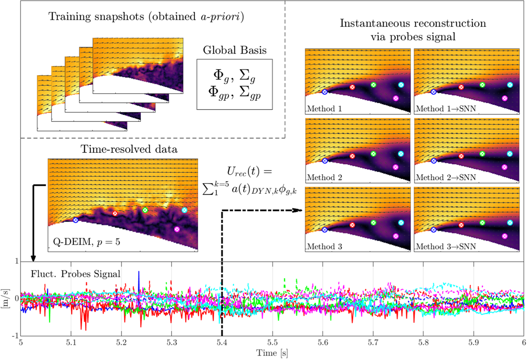
Figure 3. Conceptual illustration of the instantaneous reconstruction methodology using  $ p=5 $ probes and Q-DEIM placement. The global basis is obtained a priori and the real-time probe signals are used to approximate the instantaneous fields. The probe signals are shown with a solid line for $ {u}^{\prime } $ and dashed for $ {v}^{\prime } $ and color-coded according to their indicated locations. The total velocity shown in the plots are calculated by summing the mean and fluctuating fields. See Sections 3.3 and 3.4 for details of the methods.

Figure 4. Block diagram of the reconstruction starting from the probe signal  $ {\mathrm{U}}_p $.
3.3.1. Method 1: Sparse recovery reconstruction
The first method used is the most common implementation of sparse recovery originating from the compressed sensing literature (Donoho, Reference Donoho2006; Candès and Wakin, Reference Candès and Wakin2008; Callaham et al., Reference Callaham, Maeda and Brunton2019). This method allows to calculate a set of coefficients that approximate the real coefficients by taking advantage of the fact that many entries of the global basis are negligibly small (c.f. Jayaraman et al., Reference Jayaraman, Al Mamun and Lu2019). With this method, the POD coefficients are estimated by projecting the probes signal into a sparse basis corresponding to the global POD modes evaluated at the locations of the probes
 $$ {\boldsymbol{A}}_p^{\left[1\right]}={\boldsymbol{U}}_p{\boldsymbol{\Theta}}^{-1}, $$
where the bracketed superscript denotes the method used. Here,  $ \boldsymbol{\Theta} $ is the sparse basis formed by the product of the global basis with the sparse matrix $ \boldsymbol{\Theta} ={\boldsymbol{\Phi}}_g\boldsymbol{C} $. The number of rows in $ {\boldsymbol{A}}_p $ corresponds to the number of samples (rows) of $ {\boldsymbol{U}}_p $, and the number of columns is the number of probe modes. As we center our analysis around the Q-DEIM placement method described in Section 3.2, the sparse basis $ \boldsymbol{\Theta} $ is a square matrix with the number of probes $ p $ equal to the number of reconstruction modes $ k $.
As mentioned in Section 3.2, the optimal locations of the probes are the locations within  $ {\boldsymbol{\Phi}}_g $ that minimize the matrix condition number of $ \boldsymbol{\Theta} $. In other words, locations within the global basis with very little variance across the modes will lead to error propagation and low SNR upon the inversion in equation (5). Therefore, the best locations will correspond to the locations with the largest variance across the modes of the global basis.
3.3.2. Method 2: Extended-POD reconstruction
Motivated by studies that seek to approximate the POD coefficients using either a different variable or a separate measurement, extended POD (Borée, Reference Borée2003) offers a flexible framework with which to approximate the coefficients. (Borée, Reference Borée2003) showed that by projecting the temporal modes of one quantity into the measurements of another, one obtains a set of extended spatial modes that can be used as a basis to reconstruct the part of the measurements that is correlated to the quantity of interest. When all modes are included, this is equivalent to the well known LSE (Adrian and Moin, Reference Adrian and Moin1988; Lasagna et al., Reference Lasagna, Orazi and Iuso2013; Hosseini et al., Reference Hosseini, Martinuzzi and Noack2015).
For the present study, a framework inspired by extended POD is implemented treating the probes as a quantity to be correlated to the full flow field. If the assumption is made that the coefficients of the probes are highly correlated with the coefficients of the flow field, one can use the same training data used to calculated the global POD basis  $ {\boldsymbol{\Phi}}_g $ to produce a global probe POD basis $ {\boldsymbol{\Phi}}_{gp} $. The coefficients are then obtained as
 $$ {\boldsymbol{A}}_p^{\left[2\right]}={\boldsymbol{U}}_p{\boldsymbol{\Phi}}_{gp}^T, $$
where the transpose is used on the global probe basis as it is orthogonal by construction. The global probe basis is generated for all tested probe numbers and positions across all 9,000 training samples used to construct the global libraries. For the sake of memory allocation, only one set of random probe locations is tested to avoid calculating and storing hundreds of additional global probe libraries. It was confirmed after testing two other sets of random placements that the results presented hereafter were qualitatively unaffected.
3.3.3. Method 3: Quasi-Orthogonal extended-POD reconstruction
Building off of the methodology of the previous subsection, the quasi-orthogonal extended-POD reconstruction utilizes all of the available information from the global POD and global probe POD libraries to produce the reconstruction. Instead of simply assuming that the coefficients produced from the global probe modes will approximate the real coefficients, instead a quasi-orthogonal basis  $ {\boldsymbol{\Psi}}_p $ is calculated using the pseudoinverse of the singular values of the global probe modes $ {\boldsymbol{\Sigma}}_{gp}^{-1} $. The term “quasi” is used to emphasize that there is no guarantee that the resulting basis will be perfectly orthogonal as it is constructed using the training data and subsequently projected into by independent time-resolved testing data. The coefficients can then be approximated using the global singular values to rescale the quasi-orthogonal basis as
 $$ {\boldsymbol{A}}_p^{\left[3\right]}=\overset{{\boldsymbol{\Psi}}_p}{\overbrace{{\boldsymbol{U}}_p{\boldsymbol{\Phi}}_{gp}^T{\boldsymbol{\Sigma}}_{gp}^{-1}}}{\boldsymbol{\Sigma}}_g. $$
A similar principle was used by Discetti et al. (Reference Discetti, Raiola and Ianiro2018) to up-sample time-resolved fields using simultaneous probe signals at a higher sampling frequency.
We remark that the extended-POD methodologies presented here represent a novel departure from previous studies, for example Hosseini et al. (Reference Hosseini, Martinuzzi and Noack2015). In their case, the temporal information contained within the pressure probes were used to reconstruct the velocity fields using a basis determined by the extended spatial velocity modes. The present work, by contrast, uses the global POD basis for the reconstruction and estimates the coefficients using a separate POD basis tailored for the probes. The POD basis tailored for the specific sets of probes  $ {\boldsymbol{\Phi}}_{gp} $ is the main novelty of the present approach. As the probes themselves are velocity measurements, the underlying assumption here is in the inherent correlation between the probe velocities, their coefficients, and the full-field velocities.
3.3.4. Sign correction matrix
For the extended POD-based methods of the two previous subsections, a new global probe basis is used to obtain an approximation of the coefficients. The velocity autocorrelation of the probes (the underlying physical quantity used to calculate the POD) is missing information due to the sparsity of the probe signals. This may necessarily lead to spatial probe modes  $ {\boldsymbol{\Phi}}_{gp} $ that, when mapped to the locations of the full field modes $ {\boldsymbol{\Phi}}_g $, have opposite sign. Especially for modes corresponding to the largest singular values, this can lead to reconstructions that are anti-correlated with the true underlying velocity fields. This effect is illustrated in Figure 5, showing the first three modes for the fluctuating horizontal velocity component from the global library and the global probe library side by side for the case of 500 probes placed using Q-DEIM.
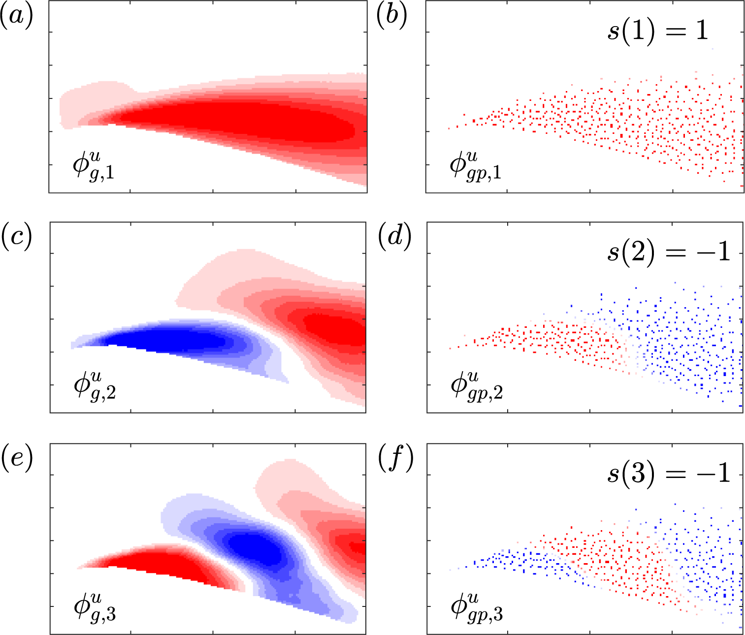
Figure 5. Global spatial modes (a, c, and e) and corresponding global spatial probe modes (b, d, and f) of  $ {u}^{\prime } $ mapped to the locations of the full field for 500 probes placed using the Q-DEIM. The colorbars range across $ \pm 3\sigma $ of the corresponding global modes $ {\phi}_{g,k}^u $ from blue to red. Modes with spatial locations that are in phase give a sign correction $ s=1 $ (a and b) and out of phase $ s=-1 $ (c–f).
To account for this effect, a sign correction matrix calculation is proposed to be calculated a priori to ensure that the two spatial bases  $ {\boldsymbol{\Phi}}_{gp} $ and $ {\boldsymbol{\Phi}}_g $ are not anticorrelated (or in other words, as correlated as possible):
 $$ s(k)=\operatorname{sgn}\left(\overline{{\boldsymbol{\phi}}_{gp,k}\circ {\boldsymbol{\phi}}_{g,k}C}\right), $$
where the overline denotes spatial averaging across the locations of the probes and the  $ \circ $ symbol denotes the Hadamard (element-wise) product. The full diagonal (and orthogonal) sign correction matrix is then
 $$ \boldsymbol{S}=\operatorname{diag}\left(\boldsymbol{s}\right), $$
where the  $ \operatorname{diag} $ function outputs a square matrix of zeros with the entries of the vector argument $ s $ along the diagonal. The coefficients are then updated through multiplication with $ \boldsymbol{S} $ as shown in Figure 4.
3.4. SNN refinement
As outlined in Figure 4, the option to apply nonlinear refinement via a NN is explored. Here, we briefly review literature concerning NN size to frame the specific implementation utilised in this study. Early on, Cybenko (Reference Cybenko1989) provided proof for the universal approximation theorem via NNs of arbitrary width with a single hidden layer and a sigmoidal activation function. A remaining issue however was in the capability to train networks with a large number of nodes in a single layer, thereby ceding computational advantage to unsupervised methods such as POD. Further generalization of the universal approximation theorem was later shown for different activation functions and multiple layers (Hornik, Reference Hornik1991). In combination with new training methods, the differences between networks of a single layer with many nodes or multiple layers with less nodes has since faded (Hinton et al., Reference Hinton, Osindero and Teh2006). Deep NNs with multiple layers remain commonplace, however, fewer layers can provide similar results taking advantage of modern hardware and training methods to significantly reduce the required training. Although single layer NNs are easier to interpret, it has been shown that networks with two layers provide better generalization capabilities (Thomas et al., Reference Thomas, Petridis, Walters, Gheytassi and Morgan2017). Networks with few layers are typically less sensitive to the specific choices of hyperparameters than their deep counterparts. As such, a SNN is adopted for the present study.
We apply an SNN architecture as outlined in the work of Erichson et al. (Reference Erichson, Mathelin, Yao, Brunton, Mahoney and Kutz2019). In general, we seek a function  $ \mathit{\mathcal{F}} $ that consists of multiple fully connected or convolutional layers with associated scalar nonlinear activation functions $ g $ and weights $ \boldsymbol{W} $ applied to input $ \boldsymbol{A} $
 $$ \mathit{\mathcal{F}}\left(\boldsymbol{A};\boldsymbol{W}\right)\hskip1.5pt := \hskip1.5pt {\boldsymbol{W}}_Lg\left({\boldsymbol{W}}_{L-1}g\left({\boldsymbol{W}}_{L-2}\cdots g\left({\boldsymbol{W}}_1\boldsymbol{A}\right)\right)\right), $$
where a shallow network has a small number of layers  $ L $. For the present study, $ L=3 $ is used, where two layers are hidden and followed by an output layer. Due to the spatial sparsity of the inputs in the present study, we favor the fully connected layers over the convolutional layers in line with similar investigations (Erichson et al., Reference Erichson, Mathelin, Yao, Brunton, Mahoney and Kutz2019; Nair and Goza, Reference Nair and Goza2019).
For the SNN architecture, shown in Table 1, we construct a first “imagination” layer with  $ 1.5p $ nodes followed by a $ 1.2p $ “refinement” layer with a 5% dropout layer in between to improve the generalization (Erichson et al., Reference Erichson, Mathelin, Yao, Brunton, Mahoney and Kutz2019). As the network scales with the input size $ p $, the amount of trainable parameters varies significantly for different networks considering varying amounts of probes. The training data however have a consistent amount of samples. This requires the larger networks to utilize additional generalization. This is achieved by the 5% dropout layer (and leaves the small networks largely unaffected). The final linear layer contains the same number of inputs (number of probes/modes) as outputs. For the activation functions, the rectified linear unit function (ReLU) is used for the hidden layers and a linear function for the output layer. The optimization is performed using the Adaptive Moment Estimation (ADAM) adaptive moment optimization (Kingma and Ba, Reference Kingma and Ba2014). The learning rate is set to 0.001, with the exponential decay rate for the first moment estimates equal to 0.9 and the exponential decay rate for the second moment estimates equal to 0.999. For numerical stability, the recommended $ \hat{\varepsilon}={10}^{-7} $ value is used.
Table 1. The neural network architecture.
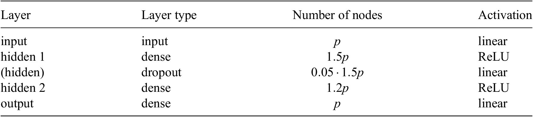
The dropout layer is only active during training.
The same training data used to obtain the POD basis,  $ {\boldsymbol{\Phi}}_g $ is used to train each NN $ \mathit{\mathcal{F}} $ using 89% of the samples $ n=8,000 $, reserving $ m=1,000 $ random samples for iterative learning validation. As demonstrated by Guastoni et al. (Reference Guastoni, Güemes, Ianiro, Discetti, Schlatter, Azizpour and Vinuesa2020), the NN for the present study is trained to recover the POD coefficients. The global coefficients for training the outputs are obtained as $ {\boldsymbol{A}}_{\boldsymbol{g}}={\boldsymbol{U}}_g{\boldsymbol{\Phi}}_g^T $ up to $ k=p $ modes (where $ p $ is the number of probes), and the sparse probe coefficients $ {\boldsymbol{A}}_{gp}^{\left[i\right]} $ using the $ i $th linear method applied to the training data $ {\boldsymbol{U}}_g\boldsymbol{C} $ as the inputs. For each set of probe locations and for each linear method, a separate network and corresponding set of weights is trained to minimize the loss
 $$ \boldsymbol{W}=\underset{\tilde{\boldsymbol{W}}}{\arg \hskip0.1em \min}\hskip0.1em \boldsymbol{\mathcal{L}}\left(\tilde{\boldsymbol{W}}\right), $$
where the loss is defined for each epoch  $ q $ as
 $$ {\boldsymbol{\mathcal{L}}}^{(q)}\left(\tilde{\boldsymbol{W}}\right)=\sum \limits_{j=1}^n{\left\Vert {\boldsymbol{A}}_g\left({t}_j\right)-\tilde{\mathit{\mathcal{F}}}\Big({\boldsymbol{A}}_{gp}^{\left[i\right]}\left({t}_j\right);\tilde{\boldsymbol{W}}\Big)\right\Vert}_1, $$
where  $ \boldsymbol{A}\left({t}_j\right) $ indicates the vector of coefficients corresponding to the $ j $th training sample and the $ \tilde{\cdot} $ indicates a dummy function or variable used for training. The $ {l}_1 $ norm is chosen in this study for evaluating the loss as it was found to outperform the commonly used $ {l}_2 $ norm. The use of the $ {l}_1 $ norm (in combination with unscaled coefficients, as will be discussed) aids the network in prioritizing an error reduction on the coefficients corresponding to the modes with larger singular values. In an effort to maintain the singular value scaling of the corresponding temporal modes, the coefficient inputs and outputs are not scaled to a zero-to-one range as is often done to speed up learning. This appears to have a minor influence on the training; only effecting initial optimization epochs where the optimizer must adjust before reducing the loss (Figure 6). The use of batch normalization for generalization was omitted and instead large batches of 3,000 samples were used. These have the added benefit of speeding up training. Other methods such as layer activation regularization or layer weight regularization were explored but were found to produce less consistent results over the various NNs without repetitive hyperparameter optimization.

Figure 6. Normalized training and validation loss  $ {\mathrm{\mathcal{L}}}^{(q)}/{\mathrm{\mathcal{L}}}^{(1)} $ within the SNN for Method 1 using 5 and 500 probes and Q-DEIM placement versus number of epochs $ q $ (a) and number of epochs before stopping $ {q}_{stop} $ versus number of probes for Method 1 for each placement (b).
It is possible to include additional constraints on the loss function in equation (11) in order to keep the network more generalized (Erichson et al., Reference Erichson, Mathelin, Yao, Brunton, Mahoney and Kutz2019; Sun and Wang, Reference Sun and Wang2020). Instead for this study, early stopping was opted for to avoid overfitting. The trained network was evaluated on the validation subset every epoch and for every iteration where the loss decreased the weights were stored. If the network did not experience a new minimum in the validation loss within 500 epochs, the training was halted and the last stored weights adopted. The value of 500 was chosen ad-hoc for this particular study as it was found to strike a balance between “kick-starting” the network with enough initial epochs but was large enough to revert any apparent overfitting. This is shown in Figure 6a for  $ p=5 $ and $ 500 $ probes via input coefficients from Method 1. With this architecture and early stopping criterion, the number of epochs was on the order of a few thousand, increasing with increasing probes to a maximum of approximately 10,000 epochs (Figure 6b).
We remark that the reconstructions use the same number of modes as probes, therefore for the present study, the more probes used for the inputs the greater the performance ceiling for the SNN (up to the limit of the real coefficients truncated at  $ p $ modes).
3.5. Quantification
Two metrics are utilized to quantify the reconstruction accuracy in the present study. To quantify the phase properties of the reconstruction, the normalized correlation is defined as
 $$ {\rho}_{u^{\prime }}=\frac{\left\langle {u}^{\prime}\left( x,t\right){u}_{rec}^{\prime}\left( x,t\right)\right\rangle }{{\left\langle {u}^{\prime }{\left( x,t\right)}^2\right\rangle}^{1/2}{\left\langle {u}_{rec}^{\prime }{\left( x,t\right)}^2\right\rangle}^{1/2}}, $$
where the angled brackets  $ \left\langle \cdot \right\rangle $ indicated averaging over all space and time and here $ {u}_{rec}^{\prime } $ is the reconstruction of the horizontal fluctuating velocity. The correlation takes a value of 1 for a reconstruction that is completely in phase, −1 when it is out of phase, and 0 when it is uncorrelated. To evaluate the overall difference between the original and reconstructed fields, the root-mean-square error is defined as
 $$ {e}_{u^{\prime }}=\frac{{\left\langle {\left({u}^{\prime}\left( x,t\right)-{u}_{rec}^{\prime}\left( x,t\right)\right)}^2\right\rangle}^{1/2}}{{\left\langle {u}^{\prime }{\left( x,t\right)}^2\right\rangle}^{1/2}}. $$
The root-mean-square error describes the fraction by which the reconstruction differs from the original fields, with a perfect reconstruction at  $ e=0 $. Equations (13) and (14) are analogously defined for the vertical fluctuations $ {v}^{\prime } $.
4. Results
The results are presented first using the linear methods alone, followed by with nonlinear SNN refinement as outlined in Section 3 and Figure 4. The reconstructions evaluate the ability of the linear and nonlinear methods to predict instantaneous flow fields using the testing data consisting of 5,468 samples. For all results, the number of modes  $ k $ used in the reconstructions is equal to the number of probes $ p $. This was chosen based on the underlying principles of the calculation for the optimal placement using the Q-DEIM (see Section 3.2); revealing optimal probe locations for reconstruction Method 1 specifically (Section 3.3.1). These were found to correspond to locations within the separated region of the flow (Figure 5). We remark, however, that the other linear methods (Methods 2 and 3) need not necessarily use all $ k=p $ modes in their reconstructions. For the present study, we opt to present $ k=p $ for all methods for consistency of comparison.
4.1. Linear reconstruction
The normalized root mean square error and correlations for the three linear methods are presented for each component of the fluctuating velocity in Figures 7 and 8 for Q-DEIM and random placement, respectively. The best possible performance is indicated in both figures by the reconstruction calculated using the rank-truncated POD via equation (2). It is immediately apparent that the maximum possible performance with the maximum number of probes  $ p=500 $ corresponds to a normalized root mean square error of 16 and $ 24\% $ and correlations of $ 0.99 $ and $ 0.96 $ for $ {u}^{\prime } $ and $ {v}^{\prime } $, respectively. This highlights the challenge of applying a reduced order model such as POD to a turbulent flow as in the present case; resulting in many required modes to capture the fluctuations.

Figure 7. Normalized root mean square error (a and b) and correlations (c and d) versus number of probes for  $ {u}^{\prime } $ (a and c) and $ {v}^{\prime } $ (b and d) using the Q-DEIM for probe placement applied to the testing data via Method 1 (squares), Method 2 (circles), Method 3 (triangles), and POD (diamonds). The number of reconstruction modes $ k $ is equal to the number of probes used $ p $. The POD-based reconstructions are obtained via equation (2) using the coefficients from projecting the full velocity fields into the global basis.
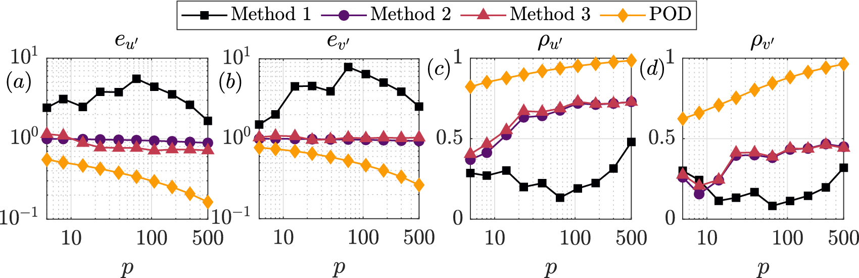
Figure 8. Normalized root mean square error (a and b) and correlations (c and d) versus number of probes for  $ {u}^{\prime } $ (a and c) and $ {v}^{\prime } $ (b and d) using random probe placement applied to the testing data from via Method 1 (squares), Method 2 (circles), Method 3 (triangles), and proper orthogonal decomposition (POD; diamonds). The number of reconstruction modes $ k $ is equal to the number of probes used $ p $. The POD-based reconstructions are obtained via equation (2) using the coefficients from projecting the full velocity fields into the global basis.
The results in Figure 7 highlight the differences in the three proposed methods when the probes are placed using Q-DEIM. For this placement, the sparse recovery via Method 1 significantly outperforms the other methods. At 500 probes, Method 1 was able to recover the spatio-temporal fluctuations to within 25 and 40% for  $ {u}^{\prime } $ and $ {v}^{\prime } $, respectively, with correlations exceeding 90%. The relative superiority of Method 1 is enforced by construction, as the Q-DEIM ensures that Method 1 produces coefficients that most efficiently sample the POD basis. Methods 2 and 3 show mixed results. These approaches were only able to recover the fluctuations with approximately 75% error for $ {u}^{\prime } $ and even exceeding 100% for $ {v}^{\prime } $ with correlations in the approximate range of 30–60%. Both methods produce reconstructions with very similar correlations. This is unsurprising, as both methods use the same global probe basis. Method 3, on the other hand, effectively contains a rescaling of the coefficients by a factor of $ {\boldsymbol{\Sigma}}_{gp}^{-1}{\boldsymbol{\Sigma}}_g $, resulting in notable differences in the root mean square error. For $ {u}^{\prime } $, this leads to comparatively lower error using Method 3. However for $ {v}^{\prime } $, Method 3 quickly compares worse to Method 2 beyond 14 probes.
We remark that although the experimental data presented are inherently limited in its accuracy and contains noise, no systematic variation of noise on the fidelity of the reconstructions is presented. This is due to the underlying assumption that the measurement noise is largely confined to low-energy high-rank structure that was explicitly treated for in the data postprocessing (Section 2.2). The cut-off mode number for treating the random noise was found to be higher than the maximum number of modes tested for the sparse reconstructions. Nevertheless, the limited subpixel accuracy of the PIV (Adrian et al., Reference Adrian, Adrian and Westerweel2011) should be considered in the interpretation of the results. As can be seen in Figure 8, the vertical velocity fluctuation  $ {v}^{\prime } $ was found to be consistently more difficult to reconstruct across methods. This is likely due to the reduced SNR of $ {v}^{\prime } $ in the measurements, for which the vertical fluctuations span a smaller range of pixel values (average deviation $ {\sigma}_{std,v}=1.2 $ pixels) than the horizontal ( $ {\sigma}_{std,u}=1.8 $ pixels) and are therefore more greatly effected by subpixel accuracy in the PIV.
An interesting shift in the results occurs for when the probes are placed randomly as shown in Figure 8. The sparse recovery approach of Method 1 now performs significantly worse than Methods 2 and 3. This is due to the fact that the random probes have some locations outside of the shear layer. These locations contribute very little variance to the global POD basis, and when they are inverted (equation (5)) the singular values become large and amplify the noise as a result. This points to the necessity that reconstructions obtained via Method 1 must avoid probe locations with very little variance across the global basis. For the case of a separated aerofoil, this means avoiding probes outside of the separated region. On the other hand, the random placement does not greatly impact the extended–POD-based Methods 2 and 3. Both methods perform similarly between the random and Q-DEIM placements; suggesting they may be more robust to arbitrary placement. Methods 2 and 3 do not suffer from the same effect as Method 1 because they use an independent global probe basis that is tailored to the sets of probe locations using individual PODs obtained a priori.
The extended-POD methods appear more robust for the present PIV data of a separated aerofoil at high Reynolds number, but a natural question to ask is whether such robustness extends to the laminar case. To assess this, we use the DNS data of a laminar cylinder in crossflow at  $ {Re}_D=100 $ provided by Brunton and Kutz (Reference Brunton and Kutz2019) and perform sparse reconstructions of the vorticity as described by Manohar et al. (Reference Manohar, Brunton, Kutz and Brunton2018). A brief outline of the analysis is as follows. The laminar data consists of 151 snapshots for which the mean is subtracted to isolate the fluctuations. The first 100 snaphots are used to generate the global basis and the global probe basis using POD for both Q-DEIM and random placements (see Figure 1c). The remaining 51 snapshots are used for assessing the reconstructions quantified using the same metrics as the present study (Section 3.5).
The comparison to the laminar cylinder is presented in Figure 9. The results from the laminar cylinder are shown with unfilled symbols and from the present study for  $ {u}^{\prime } $ with filled symbols using Q-DEIM and random placement. Method 1 outperforms Methods 2 and 3 for reconstructing the laminar cylinder for all probe numbers and locations. Interestingly, for very few probes ( $ p=7 $), Methods 2 and 3 correlate reasonably well for the Q-DEIM placement around the cylinder. However, as the number of probes increases the correlation rapidly drops off. It is observed that as the number of probes increases, the optimal locations for the probes shift from within the wake region to concentrating near the leading edge of the cylinder. This appears to negatively impact the ability for extended POD to capture the correlation between probes and flow. The random placement however appears to give improved correlations for Methods 2 and 3 compared to the Q-DEIM; indicating that the extended POD benefits from the dispersed probe locations.

Figure 9. Comparison of normalized reconstruction correlation (a and b) and root mean square error (c and d) for the reconstruction of  $ {u}^{\prime } $ in the present case (filled symbols, $ x={u}^{\prime } $) to the laminar cylinder at $ {Re}_D=100 $ from the DNS of Brunton and Kutz (Reference Brunton and Kutz2019) (unfilled symbols, $ x=\omega $) versus number of probes using Q-DEIM (a and c) and random placement (b and d) via Method 1 (squares), Method 2 (circles), and Method 3 (triangles).
The comparison between the reconstructions in the present study and with the laminar cylinder indicates that the compressed sensing methodology is superior for systems captured by relatively few modes. This is because the compressed sensing methodology does not rely on underlying correlations between probes, but rather how their location contributes to the global basis and its corresponding sparse inversion. By contrast, the improvement in the extended–POD-based methods between Q-DEIM and randomly placed probes suggests that the extended POD relies more heavily on the underlying spatial correlations captured by the POD of the global probe basis. Indeed, it was confirmed (not shown) that spatially concentrated probes in the wake of the cylinder yielded significantly poorer reconstructions than spatially dispersed configurations. This effect may explain why the extended POD methods are more robust for the separated aerofoil; the spatially dispersed probes capture a portion of the underlying spatial correlations while the compressed sensing approach of Method 1 may be sensitive to specific regions with low variance across the global basis.
4.2. Nonlinear reconstruction
The root mean square error and correlations using the nonlinear SNN for refinement are presented in Figures 10 and 11 for the Q-DEIM and random placements, respectively. In both figures, the gray dashed lines indicate the reconstructions without applying the SNN. Regardless of which linear method is used to supply the input for the SNN, the output coefficients perform nearly identically for each placement. The Q-DEIM placement appears to slightly outperform the random placement; pointing to the importance of the underlying correlations between the input and output coefficients on their performance of the SNN. Only for very large numbers of probes using the random placement can some small differences arise between input methods (Figure 11). In any case, the SNN outperforms all of the linear methods both in terms of correlation and root mean square error. The SNNs are trained using a loss function that is designed to minimize the difference between the known POD coefficients and the output of the SNN. It is therefore unsurprising that it outperforms the linear counterparts, although it does not fully recover the true underlying POD coefficients for either placement.

Figure 10. Normalized root mean square error (a and b) and correlations (c and d) versus number of probes for  $ {u}^{\prime } $ (a and c) and $ {v}^{\prime } $ (b and d) using shallow neural network (SNN) refinement and the Q-DEIM for probe placement applied to the testing data from via Method 1 (squares), Method 2 (circles), Method 3 (triangles), and proper orthogonal decomposition (POD; diamonds). The linear results are shown in gray dashed lines with corresponding symbols. The number of reconstruction modes $ k $ is equal is the number of probes used $ p $. The POD-based reconstructions are obtained via equation (2) using the coefficients from projecting the full velocity fields into the global basis.

Figure 11. Normalized root mean square error (a and b) and correlations (c and d) versus number of probes for  $ {u}^{\prime } $ (a and c) and $ {v}^{\prime } $ (b and d) using SNN refinement and random probe placement applied to the testing data from via Method 1 (squares), Method 2 (circles), Method 3 (triangles), and proper orthogonal decomposition (POD; diamonds). The linear results are shown in gray dashed lines with corresponding symbols. The number of reconstruction modes $ k $ is equal to the number of probes used $ p $. The POD-based reconstructions are obtained via equation (2) using the coefficients from projecting the full velocity fields into the global basis.
In order to understand more about how the SNN is performing compared to the linear methods, the singular values from the estimated coefficients  $ {\boldsymbol{A}}_{DYN} $ are extracted. This separates the orthogonal temporal part of the coefficients in order to reveal the effective singular values used for the full reconstruction. This is presented for the linear methods and with SNN refinement for the case $ p=14 $ in Figure 12 for Q-DEIM and random placement. The results are seemingly counter-intuitive. For both placements, the linear Method 3 appears to most closely approximate the true singular values of the validation run; but this does not mean that it will necessarily lead to a better reconstruction. In fact, this result is unsurprising as Method 3 is constructed to have a quasi-orthogonal set of temporal probe modes that are rescaled using the global ones, and therefore will most closely resemble the true singular values upon extraction from the coefficients. The other two methods on the other hand do nothing explicit to regulate the orthogonal basis of the coefficients, and this is manifested by singular values in Figure 12 that depart from the true ones.

Figure 12. Singular values  $ {\sigma}_{A,k} $ extracted from the estimated coefficients $ {A}_{DYN} $ normalized by the leading order singular value of the true coefficients for $ p=14 $ probes using linear methods (unfilled symbols) and shallow neural network (SNN) refinement (filled symbols) via Q-DEIM (a) and random placement (b).
Regardless of the linear method used, the singular values from the output of the SNN collapse together and consistently underestimate the true ones. It is important to note that no orthogonal regularization was imposed on the SNN in its construction. Instead it simply attempts to minimize the loss function between the training inputs and the training data by adjusting the weights. As the root mean square error and correlations unilaterally improve via the SNN as shown in Figures 10 and 11, the results of Figure 12 imply that recovering the underlying temporal correlation (the phase information of the temporal modes) is inherently more important than recovering the precise singular values (at least for minimizing the imposed loss function). This becomes increasingly less important as the mode number increases, as evidenced by the sharp decrease in singular values with increasing  $ k $. This shown for the case of $ p=14 $, however, similar results were found for all probe numbers tested.
5. Conclusions
We have presented three distinct linear reconstruction methodologies and a SNN for nonlinear refinement to obtain state estimations of separated turbulent flow over a NACA 0012 aerofoil at  $ \alpha ={12}^{\circ } $ and $ {Re}_c=75,000 $ using time-resolved PIV from limited probes. Each methodology was trained using 9,000 samples of PIV training data and instantaneous sample prediction was tested using all 5,468 samples of an independent time-resolved dataset. This is the first systematic investigation of sparse reconstructions for a moderately high Reynolds number advective turbulent flow obtained via experiment.
The reconstructions were first tested through the use of linear methods alone. It was found that the performance of the linear methods depended largely on the choice of placement. When the placement was chosen carefully using the Q-DEIM, the compressed-sensing approach of Method 1 greatly outperformed the extended–POD-based approaches of Methods 2 and 3 (Figure 7). When the probes were placed randomly (Figure 8), it was found that the extended POD methods performed move favorably than the compressed sensing approach of Method 1. This was due to locations within the global POD basis outside of the shear layer with small variance causing errors in the inversion of the sparse basis for Method 1. This is illustrated clearly in Figure 13c, e, showing how the reconstruction is affected when probe locations reside in the free stream.

Figure 13. Original (a), proper orthogonal decomposition (POD)-based (b), linear via Method 1 (c and e), and nonlinear (d and f) reconstructions of the total velocity at one arbitrary instant using five probes and Q-DEIM (c and d) and random (e and f) placement with every fifth velocity vector shown for clarity. Vectors are scaled automatically with respect to their individual fields and not across panels.
In order to investigate how the methods compare for the laminar case, the extended POD methods were applied to the DNS of laminar flow over a cylinder at  $ {Re}_D=100 $ of Brunton and Kutz (Reference Brunton and Kutz2019) (Figure 9). It was found that the extended–POD-based methods rely on the underlying correlations of their global probe POD basis. When the probes were grouped closely together, the reconstructions performed more poorly. When the probes were more dispersed, the autocorrelation underlying the global probe POD basis was able to capture more features. Despite this, the compressed sensing approach of Method 1 outperformed the extended POD approaches for both Q-DEIM and random placement in the laminar case. As the laminar data did not contain measurement noise and were captured by relatively few modes, small variances within the global basis were comparatively less problematic.
Nonlinear refinement of the estimated coefficients was tested through the application of an SNN using the various linear methodologies as inputs. The performance of the SNN was found to be nearly identical regardless of the linear method used and slightly more favorable for Q-DEIM placement (Figures 10 and 11). In all cases, the SNN improved the root mean square error and correlations of the reconstructions. Interestingly, it was found that the output coefficients of the SNN did not contain singular values that most closely matched the true singular values (Figure 12). Instead, the SNN naturally placed more emphasis on the phase information of the underlying temporal correlations; leading to improved reconstruction performance.
The implications for sparse reconstructions in a rapidly evolving turbulent flow (the most common type of flow in engineering applications) based on the findings of the present study can be summarized as follows. Firstly, several hundred modes (and therefore probes) are required to capture the velocity fluctuations using POD as the global basis. This implies an extensive full-field dataset must be tabulated a priori, in this case, 18 times more samples than the maximum modes used for reconstruction (9,000 samples and 500 modes). Many fewer probes may be used for reconstructions depending on the desired accuracy for the application of interest (Figure 7). Second, the placement of the probes depends on the reconstruction method of choice. The compressed sensing approach based on sparsity (Method 1) is ideal but relies on chosen locations within the flow with high variability. The extended-POD approaches (Methods 2 and 3) are less optimal however are comparatively robust and instead depend on being spatially dispersed. Finally, the nonlinear refinement via the SNN appears to equalize the linear approaches, with only a small improvement when placed favorably. This result begs the question: why should one bother with linear methods at all? The answer again depends on the application of interest. If the objective is to reconstruct the full-field as accurately as possible our results indicate one should employ as many sensors as possible and use any linear method for the inputs to the SNN. This requires training the network with the entirety of the full-field data obtained a priori. If the application instead does not require very high accuracy, the expensive task of training a NN may be avoided in which case the differences between the linear methods become relevant once again.
This study has demonstrated the capability of linear and nonlinear methods to recover instantaneous reconstructions of the full experimental velocity fields using sparse measurements. This is visualized in Figure 13. Avenues for future work include sparse reconstructions with flow control within the sensing region (which would require a distinct global basis depending on if the flow control is active or not). A further exploration of sensitivity for variations in the system, for example, changes in the freestream velocity  $ {U}_{\infty } $ or angle of attack $ \alpha $ is warranted, as the cost of training separate global bases for variations in external conditions is undesirably high (for the present study, this implies separate training datasets on the order of thousands of samples each for each $ \alpha $). Future investigations may also explore variations of the SNN architecture, which might benefit from, for example, splitting the input coefficients into singular values and orthogonal modes and training the modes with orthogonal regularization. One challenge with promising potential is to explore obtaining a greater number of outputs (modes) from the SNN than inputs; potentially achieving reconstructions that are more accurate than the rank-truncated POD itself.
Acknowledgments
The authors wish to thank Dr. John Lawson for his technical assistance with the PIV code.
Funding Statement
We gratefully acknowledge financial support from EPSRC (Grant ref No: EP/R010900/1) and EU H2020 project HOMER (Grant Ref No: 769237).
Competing Interests
The authors declare no competing interests exist.
Data Availability Statement
Code containing the interactive plots and the presented methodologies will be made available upon publication at https://doi.org/10.5258/SOTON/D1752.
Author Contributions
Conceptualization, B.G. and D.W.C.; Methodology, D.W.C. and F.D.V.; Data curation, R.S. and D.W.C.; Data visualization, D.W.C.; Writing original draft, D.W.C. and B.G. All authors approved the final submitted draft.


 Open access
Comments
No Comments have been published for this article.