


Impact Statement
Uncertainty is everywhere in data of structural optimization and design. The goal of this paper is to help engineers and researchers efficiently solve uncertain linear optimization problems of engineering structures, in absence of information on probabilistic properties or membership functions. We quantify the uncertainties by convex polyhedron model, the generalization of the widely used interval model, which overcomes some shortages of the interval model. We present a model modification method and a vertex solution method. Our work demonstrates that the vertex solution method is effective and efficient in solving above uncertain linear optimizations. The idea is to design more reliable aerospace, mechanical, or ocean engineering structures via evaluation of the worst possible, maximum response due to uncertianties.
1. Introduction
There are many uncertainties in the design of engineering structures (Klir, Reference Klir1994; Elishakoff, Reference Elishakoff1998a), such as material properties, geometric parameters, external loads, boundary conditions, and so on. If the above uncertainties are considered, the vectors and matrices in the optimization of engineering structures turn out to be no longer deterministic. The stochastic or probabilistic method, set-theoretical method, and fuzzy theory can be used to describe those uncertainties. If the uncertain parameter is the random variable with a known probability distribution, the probabilistic methodology is preferred to deal with it. If the uncertainty parameters are complex and difficult to describe crisply, the fuzzy sets-based theory is adopted to deal with them. In the absence of such information or when there is no sufficient data available, the nonprobability convex set model is more practical and widely used in the analysis and design of engineering structures (Elishakoff, Reference Elishakoff1995; Elishakoff, Reference Elishakoff1998b).
Natural question arises: Why is there no sufficient data available? The response is as follows (Ley et al., Reference Ley, Tibolt and Fromme2020): “in 2012, IBM stated that 90% of the data available today have been generated over past 2 years,” according to Sagiroglu and Sinanc (Reference Sagiroglu and Sinanc2013). When technical companies share the data, probably by creating international data banks, sufficient data will be available to utilize the proposed methodology. This applies to the case of both small data and big data. Why? This is since in both cases, in order to make structures more reliable, information on best and worst possible performances is crucial. Indeed, if the predicted worst response exceeds the allowable level, we can be convinced that the structure will fail.
With presence of uncertain parameters, the deterministic mathematical programming problems are transformed into relevant uncertain mathematical programming problems depending on the adopted modelling technique of uncertainty. There are many studies on uncertain linear programming. For example, there are active methods and passive methods for stochastic linear programming (Sengupta et al., Reference Sengupta, Tintner and Millham1963). The active approach solves the problem by introducing new design variables. The passive method accurately or approximately estimates the characteristics of the optimal value of the objective function. Evers (Reference Evers1967) proposed a new model to introduce the terms related to random constraints into the objective function, and the comparison results showed that taking the average of the elements could lead to considerable costs. For fuzzy linear programming, Zimmermann (Reference Zimmermann1978) and Chanas (Reference Chanas1989) used fuzzy linear programming to solve the multi-objective linear programming problem Ramík (Reference Ramík1986) generalized the extension principle to set-to-set mappings to solve fuzzy optimization problems. Besides, multi-objective fuzzy linear programming has been studied in Stanciulescu et al. (Reference Stanciulescu, Fortemps, Installé and Wertz2003). Among various nonprobabilistic convex models, the interval model is more widely used (Qiu et al., Reference Qiu, Wang and Chen2006). For interval linear programming, Rohn (Reference Rohn and KLE1980, Reference Rohn1981) presented a duality theorem and various forms of optimality criteria, as well as proved the strong solvability. Chinneck and Ramadan (Reference Chinneck and Ramadan2000) proposed an algorithm of interval linear programming.
However, as one of the most widely used nonprobabilistic convex models, the interval model has obvious defects in quantifying variables. In the interval method, each uncertain variable or parameter is quantified by a respective interval. In the situation of multiple variables, the whole region can be regarded as a hypercube, with surfaces of the hypercube being parallel or perpendicular to all coordinate planes. Therefore, the interval model fails to reflect the possible dependence between variables. As a consequence, the design results are supposed to be too conservative.
This study argues that if the interval model is generalized, for example, using convex polyhedron to quantify uncertainty, the results will not be as conservative as the interval model. It can also reflect the dependence between variables, because all the variables or parameters can be described by convex polyhedron as a whole, with each surface of the convex polyhedron not necessarily being parallel or perpendicular to the coordinate plane. The comparison between the interval model and the convex polyhedron model when quantifying uncertainty is shown in Figure 1. As is observed in Figure 1, the points are samples, the cuboid representing the interval model. Figure 1 also shows the polyhedron that includes all experimental points. Obviously, the interval model is anticipated to yield more conservative results than the convex polyhedron model. This is simply because the cuboid contains a bigger volume.
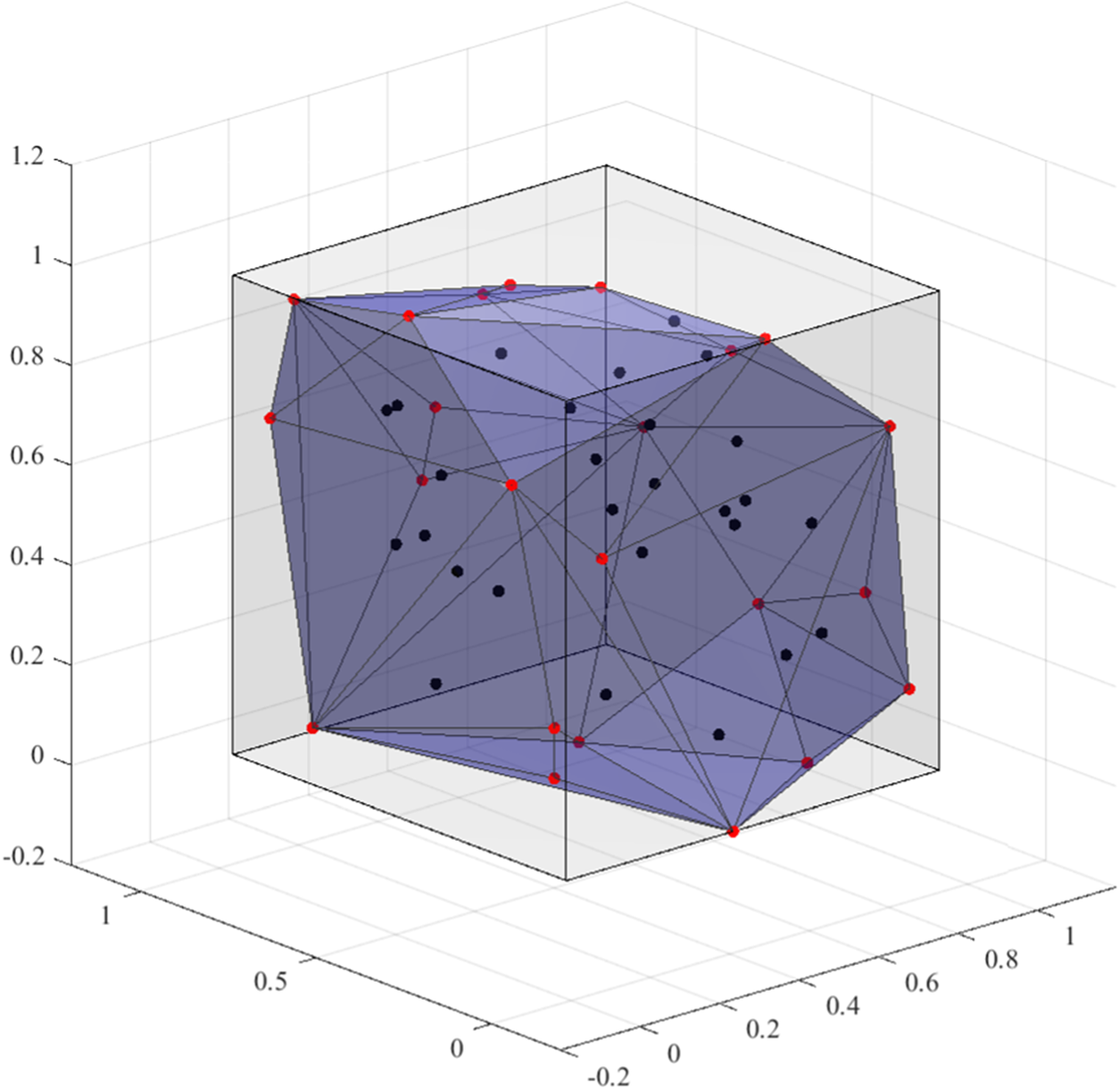
Figure 1. Comparison between interval model and convex polyhedron model.
The availability of data which will be enclosed by polyhedron is central to this investigation. In this respect, two quotes appear to be pertinent; one belongs to Galileo Galilei: “Measure what is measurable, and make measurable what is not so.” Likewise, Lord Kelvin stated “When you can measure what you are speaking about, and express it in numbers, you know something about it, when you cannot express it in numbers, your knowledge is of a meagre and unsatisfactory kind; it may be the beginning of knowledge, but you have scarcely, in your thoughts advanced to the stage of science.” Here, we use the available data without assumptions on probability density, or stationarity, or Gaussianity, or ergodicity which are frequently postulated in numerous works. According to Ley et al. (Reference Ley, Tibolt and Fromme2020), “One of the biggest misconceptions related to the Big Data phenomenon is that the sole fact of having massive data sets will solve all problems. Nothing is less true, because data do not speak by themselves (though this sentence is often incorrectly used).” In this paper, we suggest the data to be enclosed by a polyhedron and then the region to be inflated in order to anticipate future data.
The pertinent question arises on how to obtain the minimum convex polyhedron envelope of the sample points, that is, the convex hull. A variety of convex hull algorithms have been studied by present authors, such as Graham’s Scan, Divide and Conquer, Jarvis’ March, Andrew’s Monotone Chain, and Quick Hull Algorithm (Graham, Reference Graham1972; Jarvis, Reference Jarvis1973; Andrew, Reference Andrew1979; Preparata, Reference Preparata1979; Barber et al., Reference Barber, Dobkin and Huhdanpaa1996). Therefore, there is no difficulty, in principle, in introducing convex polyhedron into engineering as a new convex model to quantify uncertainty.
In addition, uncertainty problems often face the problem of solution efficiency. For the interval model with uncertainty, the vertex method is an effective method to improve the calculation efficiency. For example, Guo et al. (Reference Guo, Bai, Zhang and Gao2009) found the bounds of structural response in the truss at the vertexes of the interval set. Qiu et al. (Reference Qiu, Wang and Chen2006) and Qiu and Wang (Reference Qiu and Wang2009) presented a vertex solution to estimate the static displacement bounds and dynamic response of structures with uncertain-but-bounded parameters. The interested reader can consult also with papers by Dong and Wong (Reference Dong and Wong1985) and Dong and Shah (Reference Dong and Shah1987). The interval variation region can be regarded as a hyper-cuboid, which is a special case of the convex polyhedron. However, there is no research conducted up to now on whether the vertex method is applicable to the convex polyhedron model.
We must emphasize that there is little research on how to use convex polyhedron approach to quantify uncertainty; likewise, there is no research on the uncertain linear programming with uncertain coefficients quantified by convex polyhedron models. This paper studies the uncertain linear optimization of engineering structure in the absence of detailed sample information and focuses on the characteristics of the optimal solution set and the method of solving convex polyhedron linear programming. Section 2 introduces the uncertainty quantification method of the convex polyhedron models. Moreover, the model modification approach is employed via Chebyshev inequality, as introduced by Elishakoff and Sarlin, Reference Elishakoff and Sarlin2016. Section 3 defines the convex polyhedron-based linear programming. In Section 4, a practical vertex solution is discussed. Section 5 deals with the application of convex polyhedron linear programming in the static load-bearing capacity problem. In Section 6, some numerical examples are provided to verify the feasibility of the proposed vertex solution method.
2. Quantification of Sample Points by Convex Polyhedron Model
This section introduces the definition of a convex polyhedron and proposed the quantification method of uncertainties by convex polyhedron model.
Convex polyhedrons are common convex sets in the n-dimensional spaces. For example, convex polyhedrons in a two-dimensional space are polygons. In a three-dimensional space, a solid surrounded by four or more polygons is named a polyhedron, and when this polyhedron is on the same side of any face of itself, it can be called a convex polyhedron.
Convex polyhedrons can be expressed by the convex combination of vertex or by the intersection of appropriate half spaces (Rockafellar, Reference Rockafellar1970):
(a) If we know all the vertices  $ {\boldsymbol{x}}_i $ of a convex polyhedron, where $ {\boldsymbol{x}}_i $ is a point in an n-dimensional space
 $$ {\boldsymbol{x}}_i=\left({x}_{1,i},{x}_{2,i},\dots, {x}_{n,i}\right),\hskip0.5em i=1,2,\dots, m $$
then any point  $ \boldsymbol{x} $ in this convex polyhedron satisfies the following equality:
 $$ \boldsymbol{x}=\sum \limits_{i=1}^m{\alpha}_i{\boldsymbol{x}}_i,\hskip0.5em \left(\sum \limits_{i=1}^m{\alpha}_i=1,\hskip0.5em {\alpha}_i\hskip0.5em \ge \hskip0.5em 0,\hskip0.5em i=1,2,\dots, m\right). $$
The convex polyhedron can be expressed by the following set:
 $$ \mathcal{X}=\left\{\boldsymbol{x}:\boldsymbol{x}=\sum \limits_{i=1}^m{\alpha}_i{\boldsymbol{x}}_i,\hskip0.5em \sum \limits_{i=1}^m{\alpha}_i=1,\hskip0.5em {\alpha}_i\hskip0.5em \ge \hskip0.5em 0,\hskip0.5em i=1,2,\dots, m\right\}. $$
Figure 2 gives the example of a convex polyhedron in a two-dimensional space, inside of which point  $ \boldsymbol{x} $ can be represented as
 $$ \boldsymbol{x}=\sum \limits_{i=1}^8{\alpha}_i{\boldsymbol{x}}_i,\hskip0.5em \left(\sum \limits_{i=1}^8{\alpha}_i=1,\hskip0.5em {\alpha}_i\hskip0.5em \ge \hskip0.5em 0,\hskip0.5em i=1,2,\dots, 8\right). $$
(b) On the other hand, any point in this convex polyhedron also satisfies the following inequality:
 $$ \boldsymbol{Ax}\hskip0.5em \le \hskip0.5em \boldsymbol{b}, $$
where the faces of the convex polyhedron are given by
 $$ {\displaystyle \begin{array}{l}{\boldsymbol{a}}_1\boldsymbol{x}={b}_1,\\ {}{\boldsymbol{a}}_2\boldsymbol{x}={b}_2,\\ {}\vdots \\ {}{\boldsymbol{a}}_n\boldsymbol{x}={b}_n,\end{array}} $$
then the vectors in Equations (5) and (6)
 $$ \boldsymbol{A}=\left(\begin{array}{l}{\boldsymbol{a}}_1\\ {}{\boldsymbol{a}}_2\\ {}\vdots \\ {}{\boldsymbol{a}}_n\end{array}\right),\hskip0.5em \boldsymbol{b}=\left(\begin{array}{l}{b}_1\\ {}{b}_2\\ {}\vdots \\ {}{b}_n\end{array}\right) $$
in the convex polyhedron can be expressed by the following set:
 $$ \mathcal{X}=\left\{\boldsymbol{x}:\boldsymbol{Ax}\hskip0.5em \le \hskip0.5em \boldsymbol{b}\right\}. $$
Figure 2. Example 1 of a convex polyhedron (two-dimension).
Figure 3 gives the example of a convex polyhedron in a two-dimensional space.

Figure 3. Example 2 of a convex polyhedron (two-dimension).
2.1. Quantification of sample points by convex polyhedrons
Now we can use a convex polyhedron to quantify a limited number of sample points. For the sake of simplicity, the quantification of the following two-dimensional sample points by convex polyhedron model is first considered (note that different dimensions of each sample point  $ \left({x}_i,{y}_i\right) $ may be connected). The data points are shown in Figure 4. As is stated in the introduction, the key to the quantification is to find the convex hull of the sample points. By convex hull algorithms, we can easily find the minimum convex polyhedron that envelops all data points, which is illustrated in Figure 5.

Figure 4. The set of sample points.

Figure 5. The quantification of sample points by convex polyhedron model.
2.2. Modification of the quantification results
Figure 3 provides data from conducted experiments. But there is a possibility that sample points from future experiments fall outside the existing geometric figures (Sarlin and Elishakoff, Reference Sarlin and Elishakoff2016). Figure 6 depicts some possible future experimental data, in which blue points fall inside the convex polyhedron while red points fall outside. To forecast the future data, the convex hull calculated from available data needs to be enlarged. A probability approach has been proposed to inflating the bounding figures by Chebyshev Inequality via suggestion by Elishakoff and Sarlin (Reference Elishakoff and Sarlin2016):

Figure 6. The position between hypothesized future sample points and the convex polyhedron.
(a) Produce the initial convex hull enclosing the set of points:
 $$ \mathcal{X}=\left\{\boldsymbol{x}:\boldsymbol{x}=\sum \limits_{i=1}^m{\alpha}_i{\boldsymbol{x}}_i,\hskip0.5em \sum \limits_{i=1}^m{\alpha}_i=1,\hskip0.5em {\alpha}_i\hskip0.5em \ge \hskip0.5em 0,\hskip0.5em i=1,2,\dots, m\right\} $$
or
 $$ \mathcal{X}=\left\{\boldsymbol{x}:\boldsymbol{Ax}\hskip0.5em \le \hskip0.5em \boldsymbol{b}\right\}, $$
where x denotes all the set of points.
(b) Use Chebyshev inequality to decide the magnitude of the inflation coefficient of the initial convex hull:
 $$ \forall \varepsilon >0,\hskip0.5em P\left\{{\left(\boldsymbol{S}-E\left[\boldsymbol{S}\right]\right)}^T{\boldsymbol{\varSigma}}^{-1}\left(\boldsymbol{S}-E\left[\boldsymbol{S}\right]\right)\hskip0.5em \ge \hskip0.5em \varepsilon \right\}\hskip0.5em \le \hskip0.5em \frac{n}{\varepsilon }, $$
where ε is the inflation coefficient, S denotes the set of points, E[S] represents the mean value of S, Σ is the variance–covariance matrix, and n is the dimension of this problem. If ε has been chosen, we get an ellipse (or an n-dimensional ellipsoid)  $ {E}_{ch} $ as follows
 $$ {\left(\boldsymbol{x}-E\left[\boldsymbol{S}\right]\right)}^T{\boldsymbol{\varSigma}}^{-1}\left(\boldsymbol{x}-E\left[\boldsymbol{S}\right]\right)=\varepsilon $$
(c) With the mean value of data as the center, enlarge the initial convex hull until inscribed to the ellipse  $ {E}_{ch} $. The probability of future points falling outside the new convex polyhedron should be less than $ \frac{n}{\varepsilon } $ according to Equation (11).
Notice that it is not straightforward to find the exact enlarging coefficient especially for n-dimension conditions. If we denote the enlarging coefficient as  $ k $, the volume of the n-dimensional convex polyhedron as $ {V}_p $, the volume of the n-dimensional ellipsoid as $ {V}_E $, then the coefficient can be approximately computed by
 $$ k=\sqrt[n]{V_E/{V}_p}. $$
Although the enlarged convex polyhedron is not inscribed to the ellipse in this condition, it is a practical method to obtain  $ k $ in engineering practice.
Now we apply this method to modify the original convex hull in Figure 5 and check the anticipated future data in Figure 6. The actions to be undertaken are as follows:
(a) Produce an initial convex hull.
This convex hull has been produced in Figure 5.
(b) Choose the magnitude of the inflation coefficient.
E[S] and Σ can be obtained from the initial data in Figure 4:
 $$ E\left[S\right]={\left(4.9395,4.7144\right)}^T, $$
 $$ \boldsymbol{\varSigma} =\left(\begin{array}{cc}0.62194& -0.12696\\ {}-0.12696& 1.10190\end{array}\right). $$
If we let  $ \varepsilon =8 $, the ellipse $ {E}_{ch} $ is as follows
 $$ {\left(\boldsymbol{x}-E\left[\boldsymbol{S}\right]\right)}^T{\boldsymbol{\varSigma}}^{-1}\left(\boldsymbol{x}-E\left[\boldsymbol{S}\right]\right)=8 $$
and the probability of future points outside of the ellipse will be  $ P\hskip0.5em \le \hskip0.5em 2/8=0.25 $. Figure 7 shows the ellipse.

Figure 7. The ellipse enclosing the convex hull.
(c) Enlarge the initial convex polyhedron.
Use the approximate method to calculate the enlarging coefficient:
 $$ k=\sqrt[n]{V_E/{V}_p}\hskip0.5em \approx \hskip0.5em 1.538. $$
With the enlarging coefficient  $ k $, every new point $ {\boldsymbol{x}}^{\prime } $ of the enlarged convex polyhedron can be expressed as
 $$ {\boldsymbol{x}}^{\prime }=E\left[\boldsymbol{S}\right]+k\left(\boldsymbol{x}-E\left[\boldsymbol{S}\right]\right). $$
The equations of convex polyhedron will be the following, according to Equations (9) and (10)
 $$ {\mathcal{X}}^{\prime }=\left\{{\boldsymbol{x}}^{\prime }:{\boldsymbol{x}}^{\prime }=\sum \limits_{i=1}^m{\alpha}_i{\boldsymbol{x}}_i^{\prime },\hskip0.5em \sum \limits_{i=1}^m{\alpha}_i=1,\hskip0.5em {\alpha}_i\hskip0.5em \ge \hskip0.5em 0,\hskip0.5em i=1,2,\cdots, m\right\} $$
or
 $$ {\mathcal{X}}^{\prime }=\left\{{\boldsymbol{x}}^{\prime }:\boldsymbol{A}\left[{k}^{-1}\left({\boldsymbol{x}}^{\prime }-E\left[\boldsymbol{S}\right]\right)+E\left[\boldsymbol{S}\right]\right]\hskip0.5em \le \hskip0.5em \boldsymbol{b}\right\}. $$
The result shows in Figure 8: All the future points, with certain probability, associated with the Chebyshev inequality, fall into the new convex polyhedron, as is depicted in Figure 9.

Figure 8. The enlarged convex polyhedron.

Figure 9. The position relationship between future sample points and the inflated convex polyhedron.
3. Problem Statement
The standard form of the linear programming model is as follows:
 $$ {\displaystyle \begin{array}{ll}\min & \left\{{\boldsymbol{c}}^T\boldsymbol{x}\right\}\\ {}\mathrm{s}.\mathrm{t}.& \boldsymbol{Ax}=\boldsymbol{b}\\ {}& \boldsymbol{x}\hskip0.5em \ge \hskip0.5em \mathbf{0}\end{array}}, $$
where  $ \boldsymbol{A} $ is a deterministic matrix, while $ \boldsymbol{b} $ and $ \boldsymbol{c} $ are deterministic vectors. In engineering applications, when the uncertainty of material properties, external load, and so on, cannot be neglected, uncertain parameters $ \boldsymbol{A} $, $ \boldsymbol{b} $ and $ \boldsymbol{c} $ should be used instead of deterministic ones.
In this study, for parameters with unknown but bounded uncertainties, the convex polyhedron model is introduced for quantification:
 $$ {\displaystyle \begin{array}{l}\mathcal{A}=\left\{\boldsymbol{A}:\boldsymbol{A}=\sum \limits_{i=1}^{n_A}{\alpha}_i{\boldsymbol{A}}_i,\hskip0.5em \sum \limits_{i=1}^{n_A}{\alpha}_i=1,\hskip0.5em {\alpha}_i\hskip0.5em \ge \hskip0.5em 0,\hskip0.5em i=1,2,\cdots, {n}_A\right\},\\ {}\mathcal{B}=\left\{\boldsymbol{b}:\boldsymbol{b}=\sum \limits_{j=1}^{n_b}{\beta}_j{\boldsymbol{b}}_j,\hskip0.5em \sum \limits_{j=1}^{n_b}{\beta}_j=1,\hskip0.5em {\beta}_j\hskip0.5em \ge \hskip0.5em 0,\hskip0.5em j=1,2,\cdots, {n}_b\right\},\\ {}\mathcal{C}=\left\{\boldsymbol{c}:\boldsymbol{c}=\sum \limits_{k=1}^{n_c}{\gamma}_k{\boldsymbol{c}}_k,\hskip0.5em \sum \limits_{k=1}^{n_c}{\gamma}_k=1,\hskip0.5em {\gamma}_k\hskip0.5em \ge \hskip0.5em 0,\hskip0.5em k=1,2,\cdots, {n}_c\right\},\end{array}} $$
where  $ {\boldsymbol{A}}_i $, $ {\boldsymbol{b}}_j $, and $ {\boldsymbol{c}}_k $ denote vertexes of the polyhedrons $ \mathcal{A} $, $ \mathcal{B} $, and $ \mathcal{C} $, respectively. For example, if $ {\boldsymbol{A}}_i $ is a $ m\times n $ matrix, it can be regarded as a point in $ {R}^{m\times n} $, therefore $ \mathcal{A} $ represented by $ {\boldsymbol{A}}_i $ is a polyhedron in space $ {R}^{m\times n} $.
Then, the convex polyhedron model of linear programming problem is given by
 $$ {\displaystyle \begin{array}{ll}\min & \left\{{\boldsymbol{c}}^T\boldsymbol{x}\right\}\\ {}\mathrm{s}.\mathrm{t}.& \boldsymbol{Ax}=\boldsymbol{b}\\ {}& \boldsymbol{c}\in \mathcal{C},\boldsymbol{A}\in \mathcal{A},\boldsymbol{b}\in \mathcal{B}\\ {}& \boldsymbol{x}\hskip0.5em \ge \hskip0.5em \mathbf{0}\end{array}}. $$
In which  $ \mathcal{A} $, $ \mathcal{B} $, and $ \mathcal{C} $ are quantified through Equation (22). The optimal solutions of convex polyhedron linear programming (23) should be a set denoted as $ \boldsymbol{X} $, which contains optimal solutions of determining linear programming for every $ \boldsymbol{A} $, $ \boldsymbol{b} $, and $ \boldsymbol{c} $ of $ \mathcal{A} $, $ \mathcal{B} $, and $ \mathcal{C} $, respectively:
 $$ \boldsymbol{X}=\left\{{\boldsymbol{x}}^{\ast }:{\boldsymbol{x}}^{\ast}\hskip0.5em \mathrm{is}\hskip0.5em \mathrm{an}\hskip0.5em \mathrm{optimal}\hskip0.5em \mathrm{solution}\hskip0.5em \mathrm{of}\hskip0.5em (1),\hskip0.5em \boldsymbol{c}\hskip0.5em \in \hskip0.5em \mathcal{C},\boldsymbol{A}\hskip0.5em \in \hskip0.5em \mathcal{A},\boldsymbol{b}\hskip0.5em \in \hskip0.5em \mathcal{B}\right\}. $$
4. Vertex Solution Method of Convex Polyhedron Linear Programming
In this section, the vertex solution for efficiently solving convex polyhedron linear programming (23) is discussed.
4.1. Notes about optimal solutions
For any  $ \boldsymbol{A} $, $ \boldsymbol{b} $, and $ \boldsymbol{c} $ in Equation (23), they can be expressed by the linear combination vertexes of polyhedrons $ \mathcal{A} $, $ \mathcal{B} $, and $ \mathcal{C} $:
 $$ \boldsymbol{A}=\sum \limits_{i=1}^{n_A}{\alpha}_i{\boldsymbol{A}}_i,\hskip0.5em \boldsymbol{b}=\sum \limits_{j=1}^{n_b}{\beta}_j{\boldsymbol{b}}_j,\hskip0.5em \boldsymbol{c}=\sum \limits_{k=1}^{n_c}{\gamma}_k{\boldsymbol{c}}_k. $$
According to the fundamentals of the linear programming problem, the optimal solution is obtained at the vertices of the convex set of its feasible region. As the coefficient  $ {\alpha}_i $, $ {\beta}_j $, and $ {\gamma}_k $ change, $ \boldsymbol{A} $, $ \boldsymbol{b} $, and $ \boldsymbol{c} $ as well as the optimal solution change, but the optimal solution is still obtained at the vertices of the new feasible region.
Therefore, if we choose one vertex of  $ \mathcal{A} $, $ \mathcal{B} $, and $ \mathcal{C} $ denoted as $ {\boldsymbol{A}}_i,{\boldsymbol{b}}_j $, and $ {\boldsymbol{c}}_k $ respectively, the following single linear programming model is obtained:
 $$ {\displaystyle \begin{array}{ll}\min & \left\{{\boldsymbol{c}}_k^T\boldsymbol{x}\right\}\\ {}\mathrm{s}.\mathrm{t}.& {\boldsymbol{A}}_i\boldsymbol{x}={\boldsymbol{b}}_j\\ {}& \boldsymbol{x}\hskip0.5em \ge \hskip0.5em \mathbf{0}\end{array}}. $$
One then represents the optimal solution of Equation (26) as  $ {\boldsymbol{x}}_{ijk}^{\ast } $, and solves the above linear programming problem for any combination of $ {\boldsymbol{A}}_i,{\boldsymbol{b}}_j,{\boldsymbol{c}}_k $. A set of those optimal solutions is as follows:
 $$ {\boldsymbol{X}}^v=\left\{{\boldsymbol{x}}_{ijk}^{\ast }:i=1,2,\dots, {n}_A,\hskip0.5em j=1,2,\dots, {n}_b,\hskip0.5em k=1,2,\dots, {n}_c\right\}. $$
Since the programming problem (23) is linear, it is natural to conjecture that the set of linear combinations of  $ {\boldsymbol{x}}_{ijk}^{\ast } $(denoted by $ {\boldsymbol{X}}^{\prime } $) may be used to approximately quantify the solution set $ \boldsymbol{X} $:
 $$ {\displaystyle \begin{array}{l}{\boldsymbol{X}}^{\prime }=\left\{{\boldsymbol{x}}^{\ast }:\sum \limits_{i,j,k}{\mu}_i{\nu}_j{\upsilon}_k{\boldsymbol{x}}_{ijk}^{\ast },\hskip0.5em \sum \limits_i{\mu}_i=1,\hskip0.5em \sum \limits_j{\nu}_j=1,\hskip0.5em \sum \limits_k{\upsilon}_k=1,\hskip0.5em {\mu}_i,\hskip0.5em {\nu}_j,{\upsilon}_k\hskip0.5em \ge \hskip0.5em 0,\right.\\ {}\hskip6.5em \left.i=1,\dots, {n}_A,\hskip0.5em j=1,\dots, {n}_b,\hskip0.5em k=1,\dots, {n}_c\right\}.\end{array}} $$
However, the correctness of this conjecture should be rigorously established. In Section 4.2, this conjecture is proved. In Section 4.3, a vertex solution method of convex polyhedron linear programming problem is presented.
4.2. Properties of the optimal solution set
First of all, the necessary condition for every optimal solution is proved. In Appendix A, the relation between the optimal solution set  $ \boldsymbol{X} $ and the set $ {\boldsymbol{X}}^{\prime } $ is studied.
This section studies the properties of the optimal solution and gives a necessary condition that every optimal solution of (23) should satisfy. To simplify the discussion, the following assumption is made: Small variations  $ \Delta \hskip0.2em \boldsymbol{A} $, $ \Delta \hskip0.2em \boldsymbol{b} $, and $ \Delta \hskip0.2em \boldsymbol{c} $ will change the position of the optimal solution without altering the numbers of vertices and the corresponding vertices of the optimal solution.
First of all,  $ \boldsymbol{A},\boldsymbol{b},\boldsymbol{c} $ can be expressed by the sum of nominal value and variation:
 $$ \boldsymbol{A}={\boldsymbol{A}}_0+\Delta \hskip0.2em \boldsymbol{A},\hskip0.5em \boldsymbol{b}={\boldsymbol{b}}_0+\Delta \hskip0.2em \boldsymbol{b},\hskip0.5em \boldsymbol{c}={\boldsymbol{c}}_0+\Delta \hskip0.2em \boldsymbol{c} $$
then vertices of polyhedrons  $ \mathcal{A} $, $ \mathcal{B} $, and $ \mathcal{C} $ can be written as
 $$ {\boldsymbol{A}}_i={\boldsymbol{A}}_0+\Delta \hskip0.2em {\boldsymbol{A}}_i,\hskip0.5em {\boldsymbol{b}}_j={\boldsymbol{b}}_0+\Delta \hskip0.2em {\boldsymbol{b}}_j,\hskip0.5em {\boldsymbol{c}}_k={\boldsymbol{c}}_0+\Delta \hskip0.2em {\boldsymbol{c}}_k. $$
By substitution of (30) into (22), every  $ \boldsymbol{A} $, $ \boldsymbol{b} $, and $ \boldsymbol{c} $ will be represented as follows
 $$ {\displaystyle \begin{array}{l}\boldsymbol{A}=\sum \limits_i{\boldsymbol{A}}_i=\sum \limits_i{\alpha}_i\left({\boldsymbol{A}}_0+\Delta \hskip0.2em {\boldsymbol{A}}_i\right),\\ {}\boldsymbol{b}=\sum \limits_j{\boldsymbol{b}}_j=\sum \limits_j{\beta}_j\left({\boldsymbol{b}}_0+\Delta \hskip0.2em {\boldsymbol{b}}_j\right),\\ {}\boldsymbol{c}=\sum \limits_k{\boldsymbol{c}}_k=\sum \limits_k{\gamma}_k\left({\boldsymbol{c}}_0+\Delta \hskip0.2em {\boldsymbol{c}}_k\right).\end{array}} $$
A linear programming problem for  $ {\boldsymbol{A}}_0 $, $ {\boldsymbol{b}}_0 $, and $ {\boldsymbol{c}}_0 $ is
 $$ {\displaystyle \begin{array}{ll}\min & \left\{{\boldsymbol{c}}_0^T\boldsymbol{x}\right\}\\ {}\mathrm{s}.\mathrm{t}.& {\boldsymbol{A}}_0\boldsymbol{x}={\boldsymbol{b}}_0\\ {}& \boldsymbol{x}\hskip0.5em \ge \hskip0.5em \mathbf{0}\end{array}}. $$
The optimal solution of (32) is denoted as  $ {\boldsymbol{x}}_0^{\ast } $. According to Equation (31), a linear programming problem concerning $ \boldsymbol{A} $, $ \boldsymbol{b} $, and $ \boldsymbol{c} $ can be converted to
 $$ {\displaystyle \begin{array}{ll}\min & \left\{{\left[\sum \limits_k{\gamma}_k\left({\boldsymbol{c}}_0+\Delta \hskip0.2em {\boldsymbol{c}}_k\right)\right]}^T\boldsymbol{x}\right\}\\ {}\mathrm{s}.\mathrm{t}.& \left[\sum \limits_i{\alpha}_i\left({\boldsymbol{A}}_0+\Delta \hskip0.2em {\boldsymbol{A}}_i\right)\right]\boldsymbol{x}=\sum \limits_j\hskip0.4em {\beta}_j\left({\boldsymbol{b}}_0+\Delta \hskip0.2em {\boldsymbol{b}}_j\right)\\ {}& \boldsymbol{x}\hskip0.5em \ge \hskip0.5em \mathbf{0}\end{array}}. $$
On the one hand, denote the optimal solution of (33) as  $ {\boldsymbol{x}}^{\ast } $. The variation between $ {\boldsymbol{x}}^{\ast } $ and $ {\boldsymbol{x}}_0^{\ast } $ is $ \Delta \hskip0.2em {\boldsymbol{x}}^{\ast } $
 $$ {\boldsymbol{x}}^{\ast }={\boldsymbol{x}}_0^{\ast }+\Delta \hskip0.2em {\boldsymbol{x}}^{\ast }. $$
Substitution of (34) into the constraint condition of (33), and using the constraint condition of (32), the following equation is obtained
 $$ \sum \limits_i{\alpha}_i{\boldsymbol{A}}_i{\boldsymbol{x}}^{\ast }=\sum \limits_j\hskip0.4em {\beta}_j{\boldsymbol{b}}_j. $$
On the other hand, according to the assumption in the second paragraph of this section,  $ {\boldsymbol{c}}_k $ does not affect the optimal solution. For any combination of $ {\boldsymbol{A}}_i,{\boldsymbol{b}}_j,{\boldsymbol{c}}_k $, the vertex solution of the corresponding linear programming problem is expressed as $ {\boldsymbol{x}}_{ij}^{\ast }={\boldsymbol{x}}_{0, ij}^{\ast }+\Delta \hskip0.2em {\boldsymbol{x}}_{ij}^{\ast } $. The set of $ {\boldsymbol{x}}_{ij}^{\ast } $ is denoted by
 $$ {\boldsymbol{X}}^v=\left\{{\boldsymbol{x}}_{ij}^{\ast }:i=1,2,\dots, {n}_A,\hskip0.5em j=1,2,\dots, {n}_b\right\}. $$
The linear combination of  $ {\boldsymbol{x}}_{ij}^{\ast } $ is represented by
 $$ {\boldsymbol{X}}^{\prime }=\left\{\boldsymbol{x}:\sum \limits_{i,j}{\mu}_i{\nu}_j{\boldsymbol{x}}_{ij}^{\ast },\hskip0.5em \sum \limits_i{\mu}_i=1,\hskip0.5em \sum \limits_j{\nu}_j=1,\hskip0.5em {\mu}_i\hskip0.5em \ge \hskip0.5em 0,\hskip0.5em {\nu}_j\hskip0.5em \ge \hskip0.5em 0,\hskip0.5em i=1,2,\dots, {n}_A,\hskip0.5em j=1,2,\dots, {n}_b\right\}. $$
The solution  $ {\boldsymbol{x}}_{ij}^{\ast } $ should satisfy the constraint condition:
 $$ {\boldsymbol{A}}_i{\boldsymbol{x}}_{ij}^{\ast }={\boldsymbol{b}}_j. $$
It can be shown that every optimal solution  $ {\boldsymbol{x}}^{\ast } $ can be expressed by the linear combination of vertex optimal solutions $ {\boldsymbol{x}}_{ij}^{\ast } $. The detailed demonstration is given in Appendix A. The following conclusions are drawn:
The optimal solution set  $ \boldsymbol{X} $ of convex polyhedron linear programming (23) is contained in set $ {\boldsymbol{X}}^{\prime } $:
 $$ \boldsymbol{X}\hskip0.4em \subseteq \hskip0.4em {\boldsymbol{X}}^{\prime } $$
which means that for any  $ \boldsymbol{A}\hskip0.5em \in \hskip0.5em \mathcal{A} $, $ \boldsymbol{b}\hskip0.5em \in \hskip0.5em \mathcal{B} $, and $ \boldsymbol{c}\hskip0.5em \in \hskip0.5em \mathcal{C} $, the optimal solution of the corresponding linear programming can be regarded as the linear combination of $ {\boldsymbol{x}}_{ij}^{\ast } $. Therefore, we can use $ {\boldsymbol{X}}^{\prime } $ to approximate the optimal solution set $ \boldsymbol{X} $. Furthermore, notice that $ {\boldsymbol{x}}_{ij}^{\ast } $ is not necessarily the vertex of $ {\boldsymbol{X}}^{\prime } $, but the convex hull of $ {\boldsymbol{X}}^v $ can be easily calculated to express $ {\boldsymbol{X}}^{\prime } $ in practical application:
 $$ {\boldsymbol{X}}^{\prime }= co\left({\boldsymbol{X}}^v\right). $$
Determining  $ \boldsymbol{X} $ by Equation (40) is more efficient with the help of various convex hull algorithms.
4.3. Vertex solution method
In short, the following vertex solution can be formulated for convex polyhedron linear programming:
Vertex Solution Statement: For a convex polyhedron linear programming problem (23), the optimal solution set of is approximately a polyhedron  $ \boldsymbol{X} $, the vertices of $ \boldsymbol{X} $ are elements of the set $ {\boldsymbol{X}}^v $, and $ \boldsymbol{X} $ can be expressed by the convex hull of $ {\boldsymbol{X}}^v $.
Note that we use “approximately” in the vertex solution statement, because the proof in Appendix A is based on Equation (A.4), which is a “necessary condition” of optimal solutions. Although the vertex solution statement holds approximately, the proof in Appendix A indicates that all the optimal solutions should be contained in set  $ {\boldsymbol{X}}^{\prime } $, which means no optimal solutions will be missed when using this statement.
When using the vertex solution, first we need to solve linear programming for any combination of  $ {\boldsymbol{A}}_i,{\boldsymbol{b}}_j,{\boldsymbol{c}}_k $ and obtain optimal solution $ {\boldsymbol{x}}_{ijk}^{\ast } $:
 $$ {\displaystyle \begin{array}{ll}\min & \left\{{\boldsymbol{c}}_k^T\boldsymbol{x}\right\}\\ {}\mathrm{s}.\mathrm{t}.& {\boldsymbol{A}}_i\boldsymbol{x}={\boldsymbol{b}}_j\\ {}& \boldsymbol{x}\hskip0.5em \ge \hskip0.5em \mathbf{0}\end{array}}. $$
Then set  $ {\boldsymbol{X}}^v $ can be expressed as:
 $$ {\boldsymbol{X}}^v=\left\{{\boldsymbol{x}}_{ijk}^{\ast }:i=1,2,\dots, {n}_A,\hskip0.5em j=1,2,\dots, {n}_b,\hskip0.5em k=1,2,\dots, {n}_c\right\}. $$
Finally, the optimal solution set of Equation (23) can be calculated by any convex hull algorithm:
 $$ \boldsymbol{X}\hskip0.5em \approx \hskip0.5em co\left({\boldsymbol{X}}^v\right). $$
Figure 10 gives the flow chart of the vertex solution algorithm.

Figure 10. Flow chart of vertex solution.
Note that the material in Section 4 is based on the standard form of convex polyhedron linear programming problem, which means the constraint conditions should be linear equations instead of linear inequalities. Therefore, in the subsequent numerical examples, each established convex polyhedron linear programming will be converted into the standard form.
5. Application of Convex Polyhedron Linear Programming: Static Load-Bearing Capacity Problem
In this section, the static load-bearing capacity problem of a structure is taken as an example to show how to construct a model of convex polyhedron linear programming.
The static response equation of structure is given in the standard form:
 $$ \boldsymbol{Ku}=\boldsymbol{f}, $$
where  $ \boldsymbol{K} $ is a $ n\times n $ matrix and $ \boldsymbol{u},\boldsymbol{f} $ are $ n\times 1 $ vectors. Considering the uncertainties in material and geometry, the stiffness matrix and load vector can be quantified as belonging to the convex polyhedra (the dimension should be smaller than n 2 and n, respectively). Moreover, for linear elastic structures, if only elastic modulus belongs to a convex polyhedron $ \boldsymbol{\mathcal{E}} $, the convex polyhedral dimensions of the stiffness matrix also belong to a convex polyhedron $ \mathcal{K} $, and the dimension of $ \mathcal{K} $ is the same as $ \boldsymbol{\mathcal{E}} $, since the stiffness matrix is linear with respect to the elastic modulus. Therefore, in the problem where only the elastic modulus is uncertain, the convex polyhedron of stiffness matrices can be converted to the convex polyhedron of the elastic modulus to improve efficiency.
Assume that the strength requirement of the structure is satisfied, and the displacements are constrained by inequality  $ \boldsymbol{u}\hskip0.5em \le \hskip0.5em {\boldsymbol{u}}_0 $. The load-bearing capacity problem can be modeled as following uncertain linear programming:
 $$ {\displaystyle \begin{array}{ll}\min & \left\{{\boldsymbol{c}}^T\boldsymbol{f}\right\}\\ {}\mathrm{s}.\mathrm{t}.& \boldsymbol{D}\boldsymbol{f}\hskip0.5em \le \hskip0.5em {\boldsymbol{u}}_0\\ {}& \boldsymbol{D}\hskip0.5em \in \hskip0.5em \mathcal{D}\\ {}& \boldsymbol{f}\hskip0.5em \ge \hskip0.5em \mathbf{0}\end{array}}, $$
where  $ \boldsymbol{D} $ is the flexibility matrix. It can be proved that $ \mathcal{D} $ can also be regarded as a convex polyhedron. A detailed demonstration is given in Appendix B. Therefore, the flexibility matrix can be approximated as a convex polyhedron, and (45) then constitutes a convex polyhedron linear programming problem. In addition, Equation (B.7) indicates that $ \boldsymbol{D} $ is approximately linear with respect to elastic modulus since $ \Delta \hskip0.2em {k}_{sj_s} $ is linear concerning the elastic modulus. This reminds us of using the convex polyhedron of the elastic modulus instead of that of a flexibility matrix in practice when only the elastic modulus is uncertain.
Furthermore, (45) can be converted to a standard form of convex polyhedron linear programming:
 $$ {\displaystyle \begin{array}{ll}\min & \left\{{\boldsymbol{c}}^T{\boldsymbol{f}}^{\prime}\right\}\\ {}\mathrm{s}.\mathrm{t}.& \boldsymbol{G}{\boldsymbol{f}}^{\prime }={\boldsymbol{u}}_0\\ {}& \boldsymbol{G}\hskip0.5em \in \hskip0.5em \mathcal{G}\\ {}& {\boldsymbol{f}}^{\prime}\hskip0.5em \ge \hskip0.5em \mathbf{0}\end{array}}, $$
 $$ \boldsymbol{G}=\left(\boldsymbol{D}\hskip0.5em \boldsymbol{I}\right),\hskip0.5em {\boldsymbol{f}}^{\prime }=\left(\begin{array}{l}\boldsymbol{f}\\ {}{\boldsymbol{f}}_0\end{array}\right),\hskip0.5em {\boldsymbol{c}}^{\prime }=\left(\begin{array}{l}\boldsymbol{c}\\ {}{\boldsymbol{c}}_0\end{array}\right), $$
where  $ \mathcal{G} $ is also a convex polyhedron because $ \boldsymbol{I} $ is an identity matrix.
In the subsequent section, two static load-bearing capacity problems of plane truss and stiffened composite plate, are provided as numerical examples.
6. Numerical Examples
Two examples will be presented to illustrate the structural optimization method through the convex polyhedron model in Section 6. The first example focuses on the modeling approach by studying the load-bearing capacity of a plane truss. The second case provides an uncertain optimization of a more complex engineering structure to show the feasibility of the proposed convex polyhedron model.
6.1. The load-bearing capacity of plane truss
The first example considers the load-bearing capacity of plane truss with displacement constraint, as shown in Figure 11. Nodes 4, 5, 8, and 9 are fixed. The y-direction load is applied at node 1. The nominal elastic modulus and cross-sectional area of each rod are 210 GPa and 1 × 10⁻⁴ m2, respectively.

Figure 11. Plane truss.
Due to the scatter in the material properties and manufacturing errors, the elastic modulus and cross-sectional area are uncertain. The sample points of elastic modulus and cross-sectional area are plotted in Figure 12, where the blue convex polyhedron is an inflated model by the method of 2.2 with the inflation coefficient  $ \varepsilon =15 $. To facilitate comparison with another method, the data in Figure 12 comes from two normal distribution:
 $$ E\sim N\left(210\hskip0.5em GPa,\hskip0.5em {10}^2\hskip0.5em {GPa}^2\right),\hskip0.5em A\sim N\left(1\times {10}^{-4}{m}^2,\hskip0.5em 1\times {10}^{-14}\hskip0.5em {m}^4\right). $$
Figure 12. Elastic modulus and cross-sectional area sample points.
The elastic moduli and cross-sectional areas can be different for each rod in this simple example.
Assume that the truss structure meets strength requirements, and the displacements of node 1 in x and y-directions are constrained. The displacement vector, load vector, and the corresponding stiffness matrix are  $ \boldsymbol{u}={\left({\boldsymbol{u}}_x,{\boldsymbol{u}}_y\right)}^T $, $ \boldsymbol{f}={\left(0,{\boldsymbol{f}}_y\right)}^T $ and $ \boldsymbol{K}=\left\{{K}_{11},{K}_{12};{K}_{21},{K}_{22}\right\} $, respectively, then we have:
 $$ \boldsymbol{Ku}=\boldsymbol{f} $$
Using flexibility matrix:
 $$ \boldsymbol{D}=\left[\begin{array}{cc}{D}_{11}& {D}_{12}\\ {}{D}_{21}& {D}_{22}\end{array}\right]={\boldsymbol{K}}^{-1}=\left[\begin{array}{cc}{K}_{22}& -{K}_{12}\\ {}-{K}_{21}& {K}_{11}\end{array}\right]/\det \left(\boldsymbol{K}\right) $$
then Equation (49) can be transformed into:
 $$ \boldsymbol{Df}=\boldsymbol{u} $$
As is shown in Section 5, the flexibility matrix can be approximated as a convex polyhedron. Let the displacement constraint be  $ \boldsymbol{u}\hskip0.5em \le \hskip0.5em {\boldsymbol{u}}_0 $, and the convex polyhedron model of the linear programming problem is as follows:
 $$ {\displaystyle \begin{array}{ll}\min & {f}_y\\ {}\mathrm{s}.\mathrm{t}.& \boldsymbol{D}\boldsymbol{f}\hskip0.5em \le \hskip0.5em {\boldsymbol{u}}_0\\ {}& \boldsymbol{D}\hskip0.5em \in \hskip0.5em \mathcal{D}\\ {}& {f}_y\hskip0.5em \ge \hskip0.5em \mathbf{0}\end{array}}. $$
Let  $ \boldsymbol{c}={\left(-1,0,0\right)}^T $ and transform (52) into the form of (23), then we have
 $$ {\displaystyle \begin{array}{ll}\min & {\boldsymbol{c}}^T{\left(\hskip0.2em ,{f}_y,{x}_1,{x}_2\right)}^T\\ {}\mathrm{s}.\mathrm{t}.& \boldsymbol{G}{\left(\hskip0.1em ,{f}_y,{x}_1,{x}_2\right)}^T={\boldsymbol{u}}_0\\ {}& \boldsymbol{G}\hskip0.5em \in \hskip0.5em \mathcal{G}\\ {}& \left(\hskip0.1em ,{f}_y,{x}_1,{x}_2\right)\hskip0.5em \ge \hskip0.5em \mathbf{0}\end{array}}. $$
In which  $ \boldsymbol{G}=\left[\begin{array}{cc}{G}_1& {G}_2\end{array}\right] $, $ {\boldsymbol{G}}_1=\left[\begin{array}{l}{D}_{12}\\ {}{D}_{22}\end{array}\right] $, $ {\boldsymbol{G}}_2=\left[\begin{array}{cc}1\times {10}^{-6}& 0\\ {}0& 1\times {10}^{-6}\end{array}\right]m/N $.
Next, we solve convex polyhedron linear programming (53) by vertex solution. First of all, using the data in Figure 11 to evaluate the convex hull of  $ {\boldsymbol{G}}_1 $. Then use the vertex solution to obtain the vertexes of the optimal solutions and the objective function values, which are listed in Table 1.
Table 1. Vertexes of optimal solutions and objective function values (×105 N).

As is shown in Table 2, the lower bound of objective function value is  $ {f}_{\mathrm{min}}^{\ast }=-117.74\hskip0.5em kN $ and the best optimal solution is $ {x}^{\ast }={\left(1.17743,1.09E-14,0.001381\right)}^T kN $, therefore the maximum load-bearing capacity is $ 117.74\hskip0.5em kN $; the upper bound of objective function value is $ {f}_{\mathrm{max}}^{\ast }=-79.29\hskip0.5em kN $ and the worse optimal value is $ {x}^{\ast }={\left(0.792884,3.39E-10,0.065673\right)}^T kN $, therefore the minimum load-bearing capacity is 79.29 kN. Figure 13 plots the convex hull of the optimal solution set. In conclusion, to meet the design requirements, the maximum load should not be higher than 79.29 kN.
Table 2. Comparison between convex polyhedron vertex solution method, interval method, and Monte-Carlo method.

Abbreviations: CPVSM, convex polyhedron vertex solution method; IM, interval method; MCM, Monte-Carlo method.

Figure 13. Convex hull of optimal solutions (×105 N).
To verify the effectiveness of our method, the Monte-Carlo simulation method was used for comparison. The elastic modulus and cross-sectional area are normally distributed in Equation (48). The load fy is chosen as the random variable, and the distribution function is obtained after 10,000 simulations as shown in Figure 14.

Figure 14. Distribution function of fy.
Table 2 gives a comparison between convex polyhedron vertex solution method (CPVSM), interval method (IM), and Monte-Carlo method (MCM). In the CPVSM method, the geometric gravity center is regarded as the nominal value of the optimal solution. In the interval method, the midpoint of the optimal solution interval is regarded as the nominal value. It is obvious that the optimal solution set of CPVSM is included in the result of the MCM from Table 2, and there is a difference between the nominal values of CPVSM and IM. Table 3 provided the quantiles of the Monte-Carlo method. It is found that the lower bound 79.29 kN and nominal value 92.27 kN obtained by the convex polyhedron method are both conservative for truss design.
Table 3. Quantiles of the Monte-Carlo method (×105 N).

6.2. The load-bearing capacity of stiffened composite plate
The stiffened composite plates composed of laminated plates and stiffeners have been widely used in aircraft structures, which not only ensures the structural strength, but also reduces the manufacturing cost. The stiffened composite plate considered in this paper is shown in Figure 15. The plate consists of one panel, two stringers, and eight stiffeners, of which two stiffeners are lower and upper ends. The lower end of the stiffened plate is fixed, and the rotational degrees of freedom and displacement perpendicular to the panel of the upper end is constrained. Uniform load acts on the upper end along the long side of the panel. The stringers and the panel are laminated plates, the sequence of laying is shown in Table 4. The stiffener material is aluminum alloy.

Figure 15. Stiffened composite plate.
Table 4. Laminated plate.

Considering the scatter of properties of laminated plates, the elastic modulus of 0° and 90° were obtained by testing a batch of standard parts, as shown in Figure 16, whose nominal values are 128 GPa and 10 GPa, respectively. In addition, suppose other properties are G12 = G13 = 5.50 GPa, G23 = 3.77 GPa, ν12 = ν13 = 0.316, ν23 = 0.3. At the same time, considering the scatter of aluminum alloy material, the elastic modulus interval is [70,75] GPa and the Poisson’s ratio is 0.33. The initial (red) convex polyhedron and the inflating ellipsoid of uncertain elastic moduli with 18 vertexes are plotted in Figure 17, and the inflation coefficient is  $ \varepsilon =5 $. The initial (red) and enlarging (blue) convex polyhedron are plotted in Figure 18. Parts of the same material have the same elastic moduli in this example.

Figure 16. Elastic modulus test results of laminated plates.

Figure 17. Initial convex polyhedron and the inflating ellipsoid of uncertain elastic moduli.

Figure 18. Initial and enlarging convex polyhedron of uncertain elastic moduli.
Assuming that the strength of the stiffened wall meets the requirements, but the compression along the long side of the panel should be limited. The plate is divided into 7,160 shell elements and the finite element model mesh is plotted in Figure 19. Figure 20 shows the displacement contour image of this stiffened composite plate with nominal parameters and the uniform load on the upper end is 100 MPa.

Figure 19. Finite element model mesh.

Figure 20. Displacement contour image of this stiffened composite plate with nominal parameters (mm).
Now concentrate on the load-bearing capacity of this plate. Taking the degrees of freedom of the upper end along the long side of the panel into consideration. Let  $ \boldsymbol{D} $ be the flexibility matrix, after the displacement constraints are considered, $ \boldsymbol{f} $ and $ {\boldsymbol{u}}_0 $ be the column vectors of equivalent load and permissible displacement respectively. $ \boldsymbol{D} $, $ \boldsymbol{f} $, and $ {\boldsymbol{u}}_0 $ only consist of components at the above degrees of freedom.
According to the finite element modal,  $ \boldsymbol{D} $ is a 287-by-287 matrix, and $ \boldsymbol{f} $ and $ {\boldsymbol{u}}_0 $ are 287-dimensional column vectors. With the finite element method, the relationship of the uniform load P and the column vector of equivalent load $ \boldsymbol{f} $ is established with a 287-dimensional column vector $ \boldsymbol{l} $ or $ \boldsymbol{c} $ as
 $$ \boldsymbol{f}=P\boldsymbol{l}\hskip0.5em or\hskip0.2em P={\boldsymbol{c}}^T\boldsymbol{f} $$
Similar to example 1, the load-bearing capacity of this stiffened composite plate can be determined by the convex polyhedron linear programming problem:
 $$ {\displaystyle \begin{array}{ll}\min & {\boldsymbol{c}}^T\boldsymbol{f}\\ {}\mathrm{s}.\mathrm{t}.& \boldsymbol{D}\boldsymbol{f}\hskip0.5em \le \hskip0.5em {\boldsymbol{u}}_0\\ {}& \boldsymbol{D}\hskip0.5em \in \hskip0.5em \mathcal{D}\\ {}& \boldsymbol{f}\hskip0.5em \ge \hskip0.5em \mathbf{0}\end{array}}. $$
And (55) can be transformed into the following problem by applying formula (54):
 $$ {\displaystyle \begin{array}{ll}\min & P\\ {}\mathrm{s}.\mathrm{t}.& \boldsymbol{Dl}P\hskip0.5em \le \hskip0.5em {\boldsymbol{u}}_0\\ {}& \boldsymbol{Dl}\hskip0.5em \in \hskip0.5em {\mathcal{D}}^{\prime}\\ {}& P\hskip0.5em \ge \hskip0.5em \mathbf{0}\end{array}}, $$
where  $ {\mathcal{D}}^{\prime } $ is the convex hull of $ \boldsymbol{Dl} $. Furthermore, by introducing new variables $ {\boldsymbol{P}}_0 $, (55) can be transformed into the following equivalent form:
 $$ {\displaystyle \begin{array}{ll}\min & {{\boldsymbol{c}}^{\prime}}^T{\boldsymbol{p}}^{\prime}\\ {}\mathrm{s}.\mathrm{t}.& \boldsymbol{G}{\boldsymbol{p}}^{\prime }={\boldsymbol{u}}_0\\ {}& \boldsymbol{G}\in \mathcal{G}\\ {}& {\boldsymbol{p}}^{\prime}\hskip0.5em \ge \hskip0.5em \mathbf{0}\end{array}}, $$
where
 $$ \boldsymbol{G}=\left(\boldsymbol{Dl},\hskip0.8em ,\boldsymbol{I}\right),\hskip0.6em {\boldsymbol{p}}^{\prime }=\left(\begin{array}{l}\boldsymbol{P}\\ {}{\boldsymbol{P}}_0\end{array}\right.),\hskip0.8em {\boldsymbol{c}}^{\prime }=\left[\begin{array}{l}1\\ {}0\end{array}\right]. $$
In which  $ \boldsymbol{I} $ is a 287-dimensional identity matrix and $ {\boldsymbol{P}}_0 $ is a 287-dimensional column vector. Similar to example 1, it is easy to prove that $ \mathcal{G} $ is a convex polyhedron. Therefore (57) is a standard form of a convex polyhedron linear programming problem.
Assuming that the permissible displacement of the plate is 10 mm, the components of  $ {\boldsymbol{u}}_0 $ can be set to 10 mm. By applying the vertex solution, only 18 linear programming procedures need to be solved. Notice that the uniform load is the target function of (57), so the convex polyhedron of optimal solutions need not be calculated. The 18 results are listed in Table 5. The nominal value of P is calculated from the geometric gravity center. The nominal value and bounds of P are listed in Table 6. From Tables 5 and 6, the upper bound of loading bearing capacity is 116.91 MPa, and the lower bound of loading bearing capacity is 88.87 MPa. Therefore, to meet the design requirements in most cases, the maximum load should not be higher than 88.87 MPa.
Table 5. Uniform loads.

Table 6. Nominal value and bounds of uniform load.

7. Conclusion
As is explained in Section 1, there is usually no sufficient data available in engineering. Among the models quantifying insufficient data, the interval model—one of the most widely used nonprobabilistic convex models—usually fails to reflect the dependence between variables. As a result, the design results turn out to be too conservative. The data-based convex polyhedron model is a natural extension of the interval model, overcoming the shortcomings of interval models and helping obtain reliable design results.
The convex polyhedron model for uncertain linear optimization of engineering structure is studied in this paper. Firstly, the convex polyhedron model for uncertainty quantification is studied. In order to prevent the data from future experiments fall outside of the convex hull, beyond certain probability, Chebyshev inequality has been applied to inflate the convex polyhedron.
Secondly, the characteristics of the optimal solution of the convex polyhedron linear programming problem are investigated. The vertex solution of convex polyhedron linear programming is discussed. The modeling method of convex polyhedron linear programming problem with the example of a load-bearing capacity problem of the structure is then introduced.
Finally, in the first example of the load-bearing problem of plane truss, the effectiveness of the vertex solution is verified by comparison with the Monte-Carlo method. In the second example of stiffened composite plates, one complex convex polyhedron linear programming is simplified into 18 linear programming tasks, which demonstrates the calculation efficiency of the vertex solution method.
Abbreviations
- CPVSM
convex polyhedron vertex solution method
- IM
interval method
- MCM
Monte-Carlo method
Author Contributions
Conceptualization, Z.Q.; Methodology, Z.Q., H.W., I.E., and D.L.; Data curation, H.W.; Data visualization, H.W. and D.L.; Writing-original draft, H.W.; Writing-review & editing, Z.Q., H.W., and I.E. All authors approved the final submitted draft.
Data Availability Statement
The data used in this work is proprietary and could not be made publicly available.
Competing Interests
The authors declare no competing interests.
Funding Statement
This work received no specific grant from any funding agency, commercial or not-for-profit sectors.
Appendix A: Relation Between Optimal Solutions and Vertex Solutions
Sample appendix content. This section analyzes whether every optimal solution  $ {\boldsymbol{x}}^{\ast } $ can be expressed by the linear combination of vertex optimal solutions $ {\boldsymbol{x}}_{ij}^{\ast } $.
We multiply both sides of by (35)  $ \sum \limits_j{\beta}_j $ and $ \sum \limits_i{\alpha}_i $ respectively. Equation (35) will be transformed into
 $$ \sum \limits_i\sum \limits_j{\alpha}_i{\beta}_j{\boldsymbol{A}}_i{\boldsymbol{x}}^{\ast }=\sum \limits_i\sum \limits_j{\alpha}_i{\beta}_j{\boldsymbol{b}}_j. $$
 We then multiply both sides of Equation (38) by  $ {\alpha}_i{\beta}_j $, and calculate the sum over i and j, the following relation is obtained
 $$ \sum \limits_i\sum \limits_j{\alpha}_i{\beta}_j{\boldsymbol{A}}_i{\boldsymbol{x}}_{ij}^{\ast }=\sum \limits_i\sum \limits_j{\alpha}_i{\beta}_j{\boldsymbol{b}}_j. $$
Then, comparing Equation (A.1) with (A.2), we obtain
 $$ \sum \limits_i\sum \limits_j{\alpha}_i{\beta}_j{\boldsymbol{A}}_i{\boldsymbol{x}}^{\ast }=\sum \limits_i\sum \limits_j{\alpha}_i{\beta}_j{\boldsymbol{A}}_i{\boldsymbol{x}}_{ij}^{\ast } $$
or in another form
 $$ \sum \limits_i\sum \limits_j{\alpha}_i{\beta}_j{\boldsymbol{A}}_i{\boldsymbol{x}}^{\ast }-\sum \limits_i\sum \limits_j{\alpha}_i{\beta}_j{\boldsymbol{A}}_i{\boldsymbol{x}}_{ij}^{\ast }=0. $$
Equations (A.3) and (A.4) are the necessary conditions that every optimal solution  $ {\boldsymbol{x}}^{\ast } $ of (23) should satisfy.
It is noteworthy that  $ {\boldsymbol{x}}^{\ast } $ is a function of $ {\alpha}_i,{\beta}_j $, therefore, the first term of (A.3) and (A.4) cannot be simplified. Considering the assumption at the beginning of 4.2, $ {\boldsymbol{x}}^{\ast } $ can be uniquely determined if $ {\alpha}_i,{\beta}_j $ are given by using (A.3) or (A.4).
This work can be done by analyzing every  $ {\boldsymbol{x}}^{\ast \prime}\hskip0.5em \in \hskip0.5em {\boldsymbol{X}}^{\prime } $ and every $ {\boldsymbol{x}}^{\ast \prime}\notin {\boldsymbol{X}}^{\prime } $. The necessary condition (A.4) will be used to check whether $ {\boldsymbol{x}}^{\ast \prime } $ may be one optimal solution of the problem (23) or not.
1.  $ \forall {\boldsymbol{x}}^{\ast \prime}\hskip0.5em \in \hskip0.5em {\boldsymbol{X}}^v\subseteq {\boldsymbol{X}}^{\prime } $.
it is obvious that  $ {\boldsymbol{x}}^{\ast \prime}\hskip0.5em \in \hskip0.5em \boldsymbol{X} $.
2.  $ \forall {\boldsymbol{x}}^{\ast \prime}\hskip0.5em \in \hskip0.5em {\boldsymbol{X}}^{\prime } $.
According to (37),  $ {\boldsymbol{x}}^{\ast \prime } $ can be determined as $ {\boldsymbol{x}}^{\ast \prime }=\sum \limits_{i_1,{j}_1}{\mu}_{i_1}{\nu}_{j_1}{\boldsymbol{x}}_{i_1{j}_1}^{\ast } $. Therefore, check the necessary condition as follow
 $$ \sum \limits_i\sum \limits_j{\alpha}_i{\beta}_j{\boldsymbol{A}}_i{\boldsymbol{x}}^{\ast \prime }-\sum \limits_i\sum \limits_j{\alpha}_i{\beta}_j{\boldsymbol{A}}_i{\boldsymbol{x}}_{ij}^{\ast }=\sum \limits_{i_1,{j}_1}\left[\sum \limits_i\left({\alpha}_i{\boldsymbol{A}}_i\right){\mu}_{i_1}{\nu}_{j_1}{\boldsymbol{x}}_{i_1{j}_1}^{\ast }-\frac{1}{n_A{n}_b}\sum \limits_i\sum \limits_j\left({\alpha}_i{\beta}_j{\boldsymbol{A}}_i{\boldsymbol{x}}_{ij}^{\ast}\right)\right]. $$
 Applying the equation  $ {\boldsymbol{A}}_i{\boldsymbol{x}}_{ij}^{\ast }={\boldsymbol{b}}_j $ and $ \sum \limits_i{\alpha}_i{\boldsymbol{A}}_i{\boldsymbol{x}}^{\ast \prime }=\boldsymbol{b} $, the second term in Equation (A.5) can be transformed into
 $$ {\displaystyle \begin{array}{c}\frac{1}{n_A{n}_b}\sum \limits_i\sum \limits_j\left({\alpha}_i{\beta}_j{\boldsymbol{A}}_i{\boldsymbol{x}}_{ij}^{\ast}\right)=\frac{1}{n_A{n}_b}\sum \limits_i\sum \limits_j{\alpha}_i{\beta}_j{\boldsymbol{b}}_j\\ {}=\frac{1}{n_A{n}_b}\sum \limits_i{\alpha}_i{\boldsymbol{A}}_i{\boldsymbol{x}}^{\ast \prime}\\ {}=\frac{1}{n_A{n}_b}\sum \limits_i{\alpha}_i{\boldsymbol{A}}_i\sum \limits_{i_2,{j}_2}{\mu}_{i_2}{\nu}_{j_2}{\boldsymbol{x}}_{i_2{j}_2}^{\ast },\end{array}} $$
where  $ {n}_A $ and $ {n}_b $ identify the number of vertices of polyhedrons $ \mathcal{A} $ and $ \mathcal{B} $, respectively. Substituting the equation above into Equation (A.5), the following result is obtained
 $$ \sum \limits_i\sum \limits_j{\alpha}_i{\beta}_j{\boldsymbol{A}}_i{\boldsymbol{x}}^{\ast \prime }-\sum \limits_i\sum \limits_j{\alpha}_i{\beta}_j{\boldsymbol{A}}_i{\boldsymbol{x}}_{ij}^{\ast }=\sum \limits_i{\alpha}_i{\boldsymbol{A}}_i\left[\sum \limits_{i_1,{j}_1}\left({\mu}_{i_1}{\nu}_{j_1}{\boldsymbol{x}}_{i_1{j}_1}^{\ast}\right)-\frac{1}{n_A{n}_b}\sum \limits_{i_1,{j}_1}\sum \limits_{i_2,{j}_2}{\mu}_{i_2}{\nu}_{j_2}{\boldsymbol{x}}_{i_2{j}_2}^{\ast}\right] $$
Therefore, Equation (A.4) holds. That is, if  $ {\boldsymbol{x}}^{\ast \prime}\hskip0.5em \in \hskip0.5em {\boldsymbol{X}}^{\prime } $, $ {\boldsymbol{x}}^{\ast \prime } $ maybe an optimal solution of (23). On the other hand, if Equation (A.4) does not hold, $ {\boldsymbol{x}}^{\ast \prime } $ does not belong to $ {\boldsymbol{X}}^{\prime } $. We use “maybe” here because (A.4) is a “necessary condition,” not a “sufficient and necessary condition”: Equation (A.4) is necessary for all optimal solutions, and there exist $ {\boldsymbol{x}}^{\ast \prime } $ satisfying Equation (A.4) is not an optimal solution of (23).
3.  $ \forall {\boldsymbol{x}}^{\ast}\notin {\boldsymbol{X}}^{\prime } $.
Assuming that  $ {\boldsymbol{x}}^{\ast \prime }=\sum \limits_{i_1,{j}_1}{\mu}_{i_1}{\nu}_{j_1}{\boldsymbol{x}}_{i_1{j}_1}^{\ast }+{\boldsymbol{x}}_{i_0{j}_0} $, where $ {\boldsymbol{x}}_{i_0{j}_0}\ne \mathbf{0} $ and $ \sum \limits_{i_1,{j}_1}{\mu}_{i_1}{\nu}_{j_1}{\boldsymbol{x}}_{i_1{j}_1}^{\ast }+{\boldsymbol{x}}_{i_0{j}_0}\hskip0.5em \ge \hskip0.5em \mathbf{0} $. The constraint condition holds as $ \sum \limits_i{\alpha}_i{\boldsymbol{A}}_i\left(\sum \limits_{i_1,{j}_1}{\mu}_{i_1}{\nu}_{j_1}{\boldsymbol{x}}_{i_1{j}_1}^{\ast }+{\boldsymbol{x}}_{i_0{j}_0}\right)=\boldsymbol{b} $. Similar to ii), the necessary condition is checked as
 $$ {\displaystyle \begin{array}{l}\sum \limits_i\sum \limits_j{\alpha}_i{\beta}_j{\boldsymbol{A}}_i{\boldsymbol{x}}^{\ast \prime }-\sum \limits_i\sum \limits_j{\alpha}_i{\beta}_j{\boldsymbol{A}}_i{\boldsymbol{x}}_{ij}^{\ast}\\ {}=\sum \limits_i\left({\alpha}_i{\boldsymbol{A}}_i\right)\left[\sum \limits_{i_1,{j}_1}\left({\mu}_{i_1}{\nu}_{j_1}{\boldsymbol{x}}_{i_1{j}_1}^{\ast }+\frac{1}{n_A{n}_b}{\boldsymbol{x}}_{i_0{j}_0}\right)-\frac{1}{n_A{n}_b}\sum \limits_{i_1,{j}_1}\sum \limits_{i_2,{j}_2}{\mu}_{i_2}{\nu}_{j_2}{\boldsymbol{x}}_{i_2{j}_2}^{\ast}\right]\\ {}=\sum \limits_i\left({\alpha}_i{\boldsymbol{A}}_i\right){\boldsymbol{x}}_{i_0{j}_0}\\ {}=\left({\boldsymbol{A}}_0+\sum \limits_i\Delta \hskip0.2em {\boldsymbol{A}}_i\right){\boldsymbol{x}}_{i_0{j}_0}.\end{array}} $$
 To satisfy Equation (A.4), it is required that  $ \left({\boldsymbol{A}}_0+\sum \limits_i\Delta \hskip0.2em {\boldsymbol{A}}_i\right){\boldsymbol{x}}_{i_0{j}_0}=\mathbf{0} $. Consider small quantities of zero order and first order:
 $$ \left\{\begin{array}{l}{\boldsymbol{A}}_0{\boldsymbol{x}}_{i_0{j}_0}=0\\ {}\Delta \hskip0.2em {\boldsymbol{A}}_i{\boldsymbol{x}}_{i_0{j}_0}=0,\hskip0.5em i=1,2,\dots, {n}_A\end{array}\right.. $$
In practice, the number of vertices of polyhedron  $ \mathcal{A} $ calculated from samples often larger than the equation number in (A.9), which means that simultaneous Equations (A.9) have no solution. Therefore, case (3) is not true. That is, if $ {\boldsymbol{x}}^{\ast \prime}\notin {\boldsymbol{X}}^{\prime } $, $ {\boldsymbol{x}}^{\ast \prime } $ is not an optimal solution of (23).
Appendix B: Demonstration that Flexibility Matrices can be Quantified as a Convex Polyhedron
The perturbation method will be used to demonstrate that  $ \mathcal{D} $ can also be regarded as a convex polyhedron in Appendix B.
The elements of  $ \boldsymbol{K} $ and $ \boldsymbol{D} $ are denoted by $ {k}_{ij} $ and $ {d}_{ij} $, and $ {k}_{ij} $ can be expressed by
 $$ {k}_{ij}={k}_{0, ij}+\Delta \hskip0.2em {k}_{ij} $$
 The determinant of  $ \boldsymbol{K} $ is as follows:
 $$ \det \left(\boldsymbol{K}\right)=\sum \limits_{j_1,{j}_2,\cdots, {j}_n}{\left(-1\right)}^{\tau \left(\hskip-0.1em ,{j}_1{j}_2\cdots {j}_n\right)}{k}_{1{j}_1}{k}_{2{j}_2}\cdots {k}_{nj_n}, $$
where  $ \tau \left(\hskip0.21em {j}_1{j}_2\cdots {j}_n\right) $ represent the number of inversions in $ {j}_1,{j}_2,\dots, {j}_n $. Denote the algebraic cofactor of $ {k}_{ij} $ as $ {K}_{ij} $, then $ {K}_{ij} $ can be computed as:
 $$ {K}_{ij}={\left(-1\right)}^{i+j}\sum \limits_{j_1,{j}_2,\cdots, {j}_{n-1}\ne j}{\left(-1\right)}^{\tau \left(\hskip0.1em {j}_1{j}_2\cdots {j}_{n-1}\right)}{k}_{1{j}_1}\cdots {k}_{\left(i-1\right){j}_{i-1}}{k}_{\left(i+1\right){j}_{i+1}}\cdots {k}_{nj_n} $$
 We substitute (B.1) into (B.2) and (B.3). The determinant of  $ \boldsymbol{K} $ and the algebraic cofactor of $ {k}_{ij} $ are transformed into
 $$ {\displaystyle \begin{array}{l}\det \left(\boldsymbol{K}\right)=\sum \limits_{j_1,{j}_2,\dots, {j}_n}{\left(-1\right)}^{\tau \left(\hskip0.1em {j}_1{j}_2\cdots {j}_n\right)}\left[{k}_{0,1{j}_1}{k}_{0,2{j}_2}\cdots {k}_{0,{nj}_n}+\sum \limits_{s=1}^n\left(\Delta \hskip0.2em {k}_{sj_s}\prod \limits_{l\ne s}{k}_{0,{lj}_l}\right)\right.\\ {}\hskip6.7em \left.+\sum \limits_{s,t=1}^n\left(\Delta \hskip0.2em {k}_{sj_s}\Delta \hskip0.2em {k}_{tj_t}\prod \limits_{l\ne s,l\ne t}{k}_{0,{lj}_l}\right)+\cdots +\Delta \hskip0.2em {k}_{1{j}_1}\Delta \hskip0.2em {k}_{2{j}_2}\cdots \Delta \hskip0.2em {k}_{nj_n}\right]\end{array}} $$
 $$ {\displaystyle \begin{array}{l}{K}_{ij}=\sum \limits_{j_1,{j}_2,\cdots, {j}_{n-1}\ne j}{\left(-1\right)}^{i+j+\tau \left(\hskip0.1em {j}_1{j}_2\cdots {j}_{n-1}\right)}\left[{k}_{0,1{j}_1}\cdots {k}_{0,\left(i-1\right){j}_{i-1}}{k}_{0,\left(i+1\right){j}_{i+1}}\cdots {k}_{0,{nj}_n}+\sum \limits_{s=1}^n\left(\Delta \hskip0.2em {k}_{sj_s}\prod \limits_{l\ne i,l\ne s}{k}_{0,{lj}_l}\right)\right.\\ {}\hskip11.5em \left.+\sum \limits_{s,t=1}^n\left(\Delta \hskip0.2em {k}_{sj_s}\Delta \hskip0.2em {k}_{tj_t}\prod \limits_{l\ne i,l\ne s,l\ne t}{k}_{0,{lj}_l}\right)+\cdots +\Delta \hskip0.2em {k}_{1{j}_1}\cdots \Delta \hskip0.2em {k}_{\left(i-1\right){j}_{i-1}}\Delta \hskip0.2em {k}_{\left(i+1\right){j}_{i+1}}\cdots \Delta \hskip0.2em {k}_{nj_n}\right],\end{array}} $$
where the zero-order items in (B.4) and (B.5) are represented as  $ \det \left({\boldsymbol{K}}_0\right) $ and $ {K}_{0, ij} $. Combining Equations (B.4) and (B.5), $ {d}_{ji} $ can be represented as:
 $$ {d}_{ji}=\frac{K_{ij}}{\det \left(\boldsymbol{K}\right)} $$
We retain the first-order small quantities of Equation (B.6). The following expression is obtained:
 $$ {\displaystyle \begin{array}{c}{d}_{ji}=\frac{K_{0, ij}}{\det \left({\boldsymbol{K}}_0\right)}+\frac{1}{\det \left({\boldsymbol{K}}_0\right)}\sum \limits_{j_1,{j}_2,\cdots, {j}_{n-1}\ne j}\sum \limits_{s=1}^n{\left(-1\right)}^{i+j+\tau \left(\hskip0.1em {j}_1{j}_2\cdots {j}_{n-1}\right)}\left(\Delta \hskip0.2em {k}_{sj_s}\prod \limits_{l\ne i,l\ne s}{k}_{0,{lj}_l}\right)\\ {}-\frac{K_{0, mn}}{\det^2\left({\boldsymbol{K}}_0\right)}\sum \limits_{j_1,{j}_2,\cdots, {j}_n}\sum \limits_{s=1}^n{\left(-1\right)}^{\tau \left(\hskip0.1em {j}_1{j}_2\cdots {j}_n\right)}\left(\Delta \hskip0.2em {k}_{sj_s}\prod \limits_{l\ne s}{k}_{0,{lj}_l}\right)\end{array}} $$
 We denote the zero-order term and first-order small quantity as  $ {d}_{0, ji} $ and $ \Delta \hskip0.2em {d}_{ji} $. Signify $ {\boldsymbol{D}}_0={\left({d}_{0, ij}\right)}_{n\times n} $, then the flexibility matrix is written as
 $$ \boldsymbol{D}={\boldsymbol{D}}_0+{\left(\Delta \hskip0.2em {d}_{ij}\right)}_{n\times n} $$
The former term of Equation (B.8) is the inverse of the nominal matrix  $ {\boldsymbol{K}}_0 $, while the latter term is a linear combination of matrices that only contains the first-order small quantity $ \Delta \hskip0.2em {d}_{ij} $. It is obvious that the latter term is convex according to the convex property of $ \Delta \hskip0.2em {k}_{sj_s} $.


 Open access
Comments
No Comments have been published for this article.