


1. Introduction
Given a locally compact group  $G$ and a probability measure
  $\mu \in {\rm Prob}(G)$, the associated (left) random walk on
  $G$ is the Markov chain on
  $G$ whose transition probabilities are given by the measures
  $\mu * \delta _x$. The Markov operator associated to this random walk is given by
 \[ \mathcal{P}_\mu(f)(x) = \int f(gx)\,d\mu(g), \]
where  $f$ is a continuous function on
  $G$ with compact support. The Markov operator extends to a contraction on
  $L^\infty (G)$, which is unital and (completely) positive. A function
  $f \in L^\infty (G)$ is
  $\mu$-harmonic if
  $\mathcal {P}_\mu (f) = f$. We let
  ${\rm Har}(G, \mu )$ denote the Banach space of
  $\mu$-harmonic functions. The Furstenberg–Poisson boundary [Reference FurstenbergFur63b] of
  $G$ with respect to
  $\mu$ is a certain
  $G$-probability space
  $(B, \zeta )$, such that we have a natural positivity-preserving isometric
  $G$-equivariant identification of
  $L^\infty (B, \zeta )$ with
  ${\rm Har}(G, \mu )$ via a Poisson transform.
An actual construction of the Poisson boundary  $(B, \zeta )$, which is often described as a quotient of the path space corresponding to the stationary
  $\sigma$-algebra, is less important to us here than its existence, and indeed, up to isomorphisms of
  $G$-spaces, it is the unique
  $G$-probability space such that
  $L^\infty (B, \zeta )$ is isomorphic, as an operator
  $G$-space, to
  ${\rm Har}(G, \mu )$.
Under natural conditions on the measure  $\mu$, the boundary
  $(B, \zeta )$ possesses a number of remarkable properties. It is an amenable
  $G$-space [Reference ZimmerZim78], it is doubly ergodic with isometric coefficients [Reference KaimanovichKai92, Reference Glasner and WeissGW16], and it is strongly asymptotically transitive [Reference JaworskiJaw94, Reference JaworskiJaw95]. The boundary has therefore become a powerful tool for studying rigidity properties for groups and their probability-measure-preserving actions [Reference MargulisMar75, Reference ZimmerZim80, Reference Bader and ShalomBS06, Reference Burger and MonodBM02, Reference Bader and FurmanBF20].
In light of the successful application of the Poisson boundary to rigidity properties in group theory, Alain Connes suggested (see [Reference JonesJon00]) that developing a theory of the Poisson boundary in the setting of operator algebras would be the first step toward studying his rigidity conjecture [Reference ConnesCon82], which states that two property (T) ICC (that is, every nontrivial element has infinite conjugacy class) groups have isomorphic group von Neumann algebras if and only if the groups themselves are isomorphic. Further evidence for this can be seen by the significant role that Poisson boundaries play in [Reference Creutz and PetersonCP13, Reference Creutz and PetersonCP17, Reference PetersonPet15], where a related rigidity conjecture of Connes was investigated.
Poisson boundaries can more generally be defined using any Markov operator associated to a random walk. Markov operators are particular examples of normal unital completely positive (u.c.p.) maps on von Neumann algebras, and motivated by defining Poisson boundaries for discrete quantum groups, Izumi in [Reference IzumiIzu02, Reference IzumiIzu04] was able to define a noncommutative Poisson boundary associated to any normal u.c.p. map on a general von Neumann algebra. Specifically, if  $\mathcal {M}$ is a von Neumann algebra and
  $\phi : \mathcal {M} \to \mathcal {M}$ is a normal u.c.p. map, then we let
  ${\rm Har}(\phi ) = \{ x \in \mathcal {M} \mid \phi (x) = x \}$ denote the space of
  $\phi$-harmonic operators. Izumi showed that there exists a (unique up to isomorphism) von Neumann algebra
  $\mathcal {B}_\phi$ such that, as operator systems,
  ${\rm Har}(\phi )$ and
  $\mathcal {B}_\phi$ can be identified via a Poisson transform
  $\mathcal {P}: \mathcal {B}_\phi \to {\rm Har}(\phi )$. The existence of this boundary follows by showing that
  ${\rm Har}(\phi )$ can be realized as the range of a u.c.p. idempotent on
  $\mathcal {M}$ and then applying a theorem of Choi and Effros. Alternatively, the existence of the boundary follows by considering the minimal dilation of
  $\phi$ [Reference IzumiIzu12]. We include in the appendix to this paper an elementary proof based on this perspective.
There is a well-known dictionary between many analytic notions in group theory and those in von Neumann algebras. For example, states on  $\mathcal {B}(L^2(M))$ correspond to states on
  $\ell ^\infty \Gamma$, normal Hilbert
  $M$-bimodules correspond to unitary representations, etc. ([Reference ConnesCon76b, § 2], [Reference ConnesCon80]). This allows one to develop notions such as amenability and property (T) in the setting of finite von Neumann algebras. While Izumi's boundary gives a satisfactory noncommutative analogue of the Poisson boundary associated to a general random walk, an appropriate notion of a noncommutative Poisson boundary analogous to the group setting is still missing.
The main goal of this paper is to introduce a theory of Poisson boundaries for finite von Neumann algebras that we believe will fill the role envisioned by Connes. If  $M$ is a finite von Neumann algebra with a normal faithful trace
  $\tau$, and if
  $\varphi \in \mathcal {B}(L^2(M, \tau ))_*$ is a normal state such that
  $\varphi _{|M} = \tau$, then we will view
  $\varphi$ as the distribution of a ‘noncommutative random walk’ on
  $M$. To each distribution we associate a corresponding ‘convolution operator’, which is a normal u.c.p. map
  $\mathcal {P}_\varphi : \mathcal {B}(L^2(M, \tau )) \to \mathcal {B}(L^2(M, \tau ))$, such that
  $M \subset {\rm Har}(\mathcal {P}_\varphi )$. We then define the Poisson boundary of
  $M$ with respect to
  $\varphi$ to be Izumi's noncommutative boundary
  $\mathcal {B}_\varphi$ associated to
  $\mathcal {P}_\varphi$; more precisely, the boundary is really the inclusion of von Neumann algebras
  $M \subset \mathcal {B}_\varphi$, together with the Poisson transform
  $\mathcal {P}: \mathcal {B}_\varphi \to {\rm Har}(\mathcal {P}_\varphi )$.
Poisson boundaries of groups give rise to natural Poisson boundaries of group von Neumann algebras. Indeed, as already noticed by Izumi in [Reference IzumiIzu12], if  $\Gamma$ is a countable discrete group and
  $\mu \in {\rm Prob}(\Gamma )$, then the noncommutative boundary of the u.c.p. map
  $\phi _\mu : \mathcal {B}(\ell ^2 \Gamma ) \to \mathcal {B}(\ell ^2 \Gamma )$ given by
  $\phi _\mu (T) = \int \rho _\gamma T \rho _\gamma ^* \,d\mu (\gamma )$ is naturally isomorphic to the von Neumann crossed product
  $L^\infty (B, \zeta ) \rtimes \Gamma$ where
  $(B, \zeta )$ is the Poisson boundary of
  $(\Gamma, \mu )$. Thus, many of the results we obtain are not merely analogues, but are actually generalizations of results from the theory of random walks on groups.
If  $M$ is a finite factor, then under natural conditions on the distribution
  $\varphi$, for example that its ‘support’ should generate
  $M$, we show that the boundary
  $\mathcal {B}_\varphi$ is amenable/injective (Proposition 2.4), and that the inclusion
  $M \subset \mathcal {B}_\varphi$ is ‘ergodic’, that is,
  $M' \cap \mathcal {B}_\varphi = \mathbb {C}$ (Proposition 2.7). We use techniques of Foguel [Reference FoguelFog75] to obtain equivalent characterizations for when the boundary is trivial (Theorem 2.10). The double ergodicity result of Kaimanovich [Reference KaimanovichKai92] is more subtle, as, unlike in the case for groups, there is no natural ‘diagonal’ inclusion of
  $M$ into
  $\mathcal {B}_\varphi \, \overline {\otimes }\, \mathcal {B}_\varphi$. There are, however, natural notions of left and right convolution operators, so that we may naturally associate with
  $\varphi$ a second u.c.p. map
  $\mathcal {P}^{\rm o}_\varphi$ which commutes with
  $\mathcal {P}_\varphi$ (see § 3 for the precise definition of
  $\mathcal {P}^{\rm o}_\varphi$). We may then show that bi-harmonic operators are constant, a result which is equivalent to double ergodicity in the group setting.
Theorem A (Theorem 3.1 below)
Let  $M$ be a finite factor and suppose
  $\varphi$ is as above. Then we have
 \[ {\rm Har}(\mathcal{B}(L^2(M, \tau)), \mathcal{P}_\varphi) \cap {\rm Har}(\mathcal{B}(L^2(M, \tau)), \mathcal{P}^{\rm o}_\varphi) = \mathbb{C}. \]
Motivated by the question of determining whether or not  $L\mathbb {F}_\infty$ is finitely generated, Popa studied in [Reference PopaPop21a] the class of separable II
 $_1$ factors
  $M$ that are tight, that is,
  $M$ contains two hyperfinite subfactors
  $L, R \subset M$ such that
  $L$ and
  $R^{\rm op}$ together generate
  $\mathcal {B}(L^2(M))$. He conjectures in Conjecture 5.1 of [Reference PopaPop21a] that if a factor
  $M$ has the property that all amplifications
  $M^t$ are singly generated, then
  $M$ is tight. He also notes that a tight factor
  $M$ satisfies the MV property, which states that for any operator
  $T \in \mathcal {B}(L^2(M))$ the weak closure of the convex hull of
  $\{ u (JvJ) T (Jv^*J) u^* \mid u, v \in \mathcal {U}(M) \}$ intersects the scalars. Popa then asks in Problem 7.4 of [Reference PopaPop21b] and Problem 6.3 in [Reference PopaPop21c] if free group factors, or perhaps all finite factors, have the MV property. As a consequence of double ergodicity we are able to answer Popa's problem.
Theorem B (Theorem 3.3 below)
All finite factors have the MV property.
Other consequences of double ergodicity are that it allows us to show vanishing cohomology for subbimodules of the Poisson boundary (Theorem 3.5), to generalize rigidity results from [Reference Creutz and PetersonCP13] (Theorem 4.1), and to extend results of Bader and Shalom [Reference Bader and ShalomBS06] identifying the Poisson boundary of a tensor product with the tensor product of the Poisson boundaries (Corollary 4.5).
We also introduce analogues of Avez's asymptotic entropy and Furstenberg's  $\mu$-entropy in the setting of von Neumann algebras (see § 5 for these definitions). We show that the triviality of the Poisson boundary is equivalent to the vanishing of the Furstenberg entropy (Corollary 5.15). We also use entropy to extend a result of Nevo [Reference NevoNev03] to the setting of von Neumann algebras, which shows that property (T) factors give rise to an ‘entropy gap’.
Theorem C (Theorem 6.2 below)
Let  $M$ be a II
 $_1$ factor with property (T) generated by unitaries
  $u_1, \ldots, u_n$. Define the state
  $\varphi \in \mathcal {B}(L^2M)_*$ by
  $\varphi (T) = ({1}/{n}) \sum _{k = 1}^n \langle T \widehat {u_k}, \widehat {u_k} \rangle$. There exists
  $c > 0$ such that if
  $M \subsetneq \mathcal {A}$ is an irreducible inclusion of von Neumann algebras and
  $\zeta \in \mathcal {A}_*$ is any faithful normal state such that
  $\zeta _{| M} = \tau$, then
 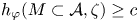 $h_\varphi (M \subset \mathcal {A}, \zeta ) \geq c$.
We end with an appendix where we construct Izumi's boundary of a u.c.p. map. Our approach is elementary, and has the advantage that it applies for general  $C^*$-algebras. This level of generality has no doubt been known by experts, but we could not find it in the current literature.
2. Boundaries
2.1 Hyperstates and bimodular u.c.p. maps
Fix a tracial von Neumann algebra  $(M, \tau )$, and suppose we have an embedding
  $M \subset \mathcal {A}$ where
  $\mathcal {A}$ is a
  $C^*$-algebra. We say that a state
  $\varphi \in \mathcal {A}^*$ is a
  $\tau$-hyperstate (or just a hyperstate if
  $\tau$ is fixed) if it extends
  $\tau$. We denote by
  $\mathcal {S}_\tau (\mathcal {A})$ the convex set of all hyperstates on
  $\mathcal {A}$. For each hyperstate
  $\varphi$ we obtain a natural inclusion
 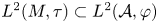 $L^2(M, \tau ) \subset L^2(\mathcal {A}, \varphi )$ induced from the map
  $x \hat {1} \mapsto x 1_{\varphi }$ for
  $x \in M$. We let
 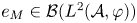 $e_M \in \mathcal {B}(L^2(\mathcal {A}, \varphi ))$ denote the orthogonal projection onto
  $L^2(M, \tau )$. We may then consider the u.c.p. map
 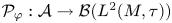 $\mathcal {P}_\varphi : \mathcal {A} \to \mathcal {B}(L^2(M, \tau ))$, defined by
 \begin{equation} \mathcal{P}_\varphi(T) = e_M T e_M,\quad T \in \mathcal{A}. \end{equation}
Note that if  $x \in M \subset \mathcal {A}$, then we have
  $\mathcal {P}_\varphi (x) = x$. We call the map
  $\mathcal {P}_\varphi$ the Poisson transform (with respect to
  $\varphi$) of the inclusion
  $M \subset \mathcal {A}$.
The following proposition is inspired by [Reference ConnesCon76b, § 2.2].
Proposition 2.1 The correspondence  $\varphi \mapsto \mathcal {P}_\varphi$ defined by (1) gives a bijective correspondence between hyperstates on
  $\mathcal {A}$, and u.c.p.,
  $M$-bimodular maps from
  $\mathcal {A}$ to
  $\mathcal {B}(L^2(M, \tau ))$. Moreover, if
  $\mathcal {A}$ is a von Neumann algebra, then
  $\mathcal {P}_\varphi$ is normal if and only if
  $\varphi$ is normal.
Also, this correspondence is a homeomorphism where the space of hyperstates is endowed with the weak $^*$ topology, and the space of u.c.p.,
  $M$-bimodular maps with the topology of pointwise weak operator topology convergence.
Proof. First note that if  $\varphi$ is a hyperstate on
  $\mathcal {A}$, then for all
  $T \in \mathcal {A}$ we have
 \[ \varphi(T)= \langle T, \hat 1 \rangle_{\varphi} = \langle \mathcal{P}_\varphi(T) \hat 1, \hat 1 \rangle_\tau. \]
From this it follows that the correspondence  $\varphi \mapsto \mathcal {P}_\varphi$ is one-to-one. To see that it is onto, suppose that
  $\mathcal {P}: \mathcal {A} \to \mathcal {B}(L^2(M, \tau ))$ is u.c.p. and
  $M$-bimodular. We define a state
  $\varphi$ on
  $\mathcal {A}$ by
  $\varphi (T) = \langle \mathcal {P}(T) \hat {1}, \hat {1} \rangle _\tau$. For all
  $y \in M$ we then have
  $\varphi (y) = \langle \mathcal {P}(y) \hat 1, \hat 1 \rangle _\tau = \tau (y)$, hence
  $\varphi$ is a hyperstate. Moreover, if
  $y, z \in M$, and
  $T \in \mathcal {A}$, then we have
 \begin{align} \langle \mathcal{P}_\varphi(T) \hat y, \hat z \rangle_\tau &= \langle \mathcal{P}_\varphi(z^* T y) \hat 1, \hat 1 \rangle_\tau \nonumber\\ &= \varphi(z^* T y)= \langle \mathcal{P}(T) \hat y, \hat z \rangle_\tau, \end{align}
hence,  $\mathcal {P}_\varphi = \mathcal {P}$.
It is also easy to check that  $\mathcal {P}_\varphi$ is normal if and only if
  $\varphi$ is.
To see that this correspondence is a homeomorphism when given the topologies above, suppose that  $\varphi$ is a hyperstate, and
  ${\varphi _\alpha }$ is a net of hyperstates. From (2) and the fact that u.c.p. maps are contractions in norm we see that
  $\mathcal {P}_{{\varphi _\alpha }}$ converges in the pointwise ultraweak topology to
  $\mathcal {P}_\varphi$ if
  ${\varphi _\alpha }$ converges weak
 $^*$ to
  $\varphi$. Conversely, setting
  $y = z = 1$ in (2) shows that if
  $\mathcal {P}_{\varphi _\alpha }$ converges in the pointwise ultraweak topology to
  $\mathcal {P}_\varphi$, then
  $\varphi _\alpha$ converges weak
 $^*$ to
  $\varphi$.
Considering the case  $\mathcal {A} = \mathcal {B}(L^2(M, \tau ))$, we see that for each hyperstate
  $\varphi$ on
  $\mathcal {B}(L^2(M, \tau ))$ we obtain a u.c.p.
  $M$-bimodular map
  $\mathcal {P}_\varphi$ on
  $\mathcal {B}(L^2(M, \tau ))$. In particular, composing such maps gives a type of convolution operation on the space of hyperstates. More generally, if
  $\mathcal {A}$ is a
  $C^*$-algebra, with
  $M \subset \mathcal {A}$, then for hyperstates
  $\psi \in \mathcal {A}^*$ and
  $\varphi \in \mathcal {B}(L^2(M, \tau ))^*$ we define the convolution
  $\varphi * \psi$ to be the unique hyperstate on
  $\mathcal {A}$ such that
 \begin{equation} \mathcal{P}_{\varphi * \psi} = \mathcal{P}_{ \varphi} \circ \mathcal{P}_{ \psi}. \end{equation}
We say that  $\psi$ is
  $\varphi$-stationary if we have
  $\varphi * \psi = \psi$, or equivalently, if
  $\mathcal {P}_\psi$ maps into the space of
  $\mathcal {P}_\varphi$-harmonic operators
 \[ {\rm Har}(\mathcal{P}_\varphi) = {\rm Har}( \mathcal{B}(L^2(M, \tau) ), \mathcal{P}_\varphi ) = \{ T \in \mathcal{B}(L^2(M, \tau) ) \mid \mathcal{P}_\varphi(T) = T \}. \]
Lemma 2.2 For a fixed  $\psi \in \mathcal {S}_\tau ( \mathcal {A} )$ the mapping
 \[ \mathcal{S}_\tau(\mathcal{B}(L^2(M, \tau))) \ni \varphi \mapsto \varphi * \psi \in \mathcal{S}_\tau(\mathcal{A}) \]
is continuous in the weak $^*$ topology.
Moreover, if  $\varphi \in \mathcal {B}(L^2(M, \tau ))_*$ is a fixed normal hyperstate, then the mapping
 \[ \mathcal{S}_\tau(\mathcal{A}) \ni \psi \mapsto \varphi * \psi \in \mathcal{S}_\tau(\mathcal{A}) \]
is also weak $^*$ continuous.


2.2 Poisson boundaries of II  $_1$ factors

Definition 2.3 Let  $\varphi \in {\mathcal {S}}_\tau ( \mathcal {B}(L^2(M, \tau )))$ be a hyperstate. We define the Poisson boundary
  $\mathcal {B}_\varphi$ of
  $M$ with respect to
  $\varphi$ to be the noncommutative Poisson boundary of the u.c.p. map
  ${\mathcal {P}}_\varphi$ as defined by Izumi [Reference IzumiIzu02], that is, the Poisson boundary
  $\mathcal {B}_\varphi$ is a
  $C^*$-algebra (a von Neumann algebra when
  $\varphi$ is normal) that is isomorphic, as an operator system, to the space of harmonic operators
  ${\rm Har}( \mathcal {B}(L^2(M, \tau ) ), \mathcal {P}_\varphi )$.
Since  $M$ is in the multiplicative domain of
  ${\mathcal {P}}_\varphi$, we see that
  $\mathcal {B}_{\varphi }$ contains
  $M$ as a subalgebra. Moreover, note that if we have a
  $C^*$-algebra
  $\mathcal {B}$, an inclusion
  $M \subseteq \mathcal {B}$ together with a completely positive isometric surjection from
  $\mathcal {B}$ to
  ${\rm Har}( \mathcal {B}(L^2(M, \tau ) ), \mathcal {P}_\varphi )$, then this induces a completely positive isometric surjection from
  $\mathcal {B}$ to
  $\mathcal {B}_{\varphi }$ which restricts to the identity on
  $M$. It is a well-known result of Choi [Reference ChoiCho72] that a completely positive surjective isometry between two
  $C^*$-algebras is a
  $\ast$-isomorphism. Thus, the Poisson boundary contains
  $M$ as a subalgebra, and the inclusion
  $(M \subset \mathcal {B}_\varphi )$ is determined up to isomorphism by the property that there exists a completely positive isometric surjection
  $\mathcal {P}: \mathcal {B}_\varphi \to {\rm Har}( \mathcal {B}(L^2(M, \tau ) ), \mathcal {P}_\varphi )$ which restricts to the identity map on
  $M$. We will always assume that
  $\mathcal {P}$ is fixed and we also call
  $\mathcal {P}$ the Poisson transform.
Given any initial hyperstate  $\varphi _0 \in \mathcal {S}_\tau ( \mathcal {B}(L^2(M, \tau ) ) )$, we may consider the hyperstate given by
  $\varphi _0 \circ \mathcal {P}$ on
  $\mathcal {B}_\varphi$. Of particular interest is the state
  $\eta$ on
  $\mathcal {B}_\varphi$ arising from the initial hyperstate
  $\varphi _0(x) \in \mathcal {S}_{\tau }(\mathcal {B}(L^2(M, \tau )))$ given by
  $\varphi _0(x)= \langle x \hat 1, \hat 1 \rangle$, which we call the stationary state on
  $\mathcal {B}_\varphi$. In this case, using (2) above, it is easy to see that we have
  $\mathcal {P}_\eta = \mathcal {P}$, and hence
  $\varphi * \eta = \eta$.
Proposition 2.4 Let  $(M, \tau )$ be a tracial von Neumann algebra and let
  $\varphi$ be a fixed hyperstate on
  $\mathcal {B}(L^2(M, \tau ))$. Then the Poisson boundary
  $\mathcal {B}_\varphi$ is injective.
Proof. If we take any accumulation point  $E$ of
  $\bigl \{ ({1}/{N}) \sum _{n = 1}^N \mathcal {P}_\varphi ^n\bigr \}_{N \in \mathbb {N}}$ in the topology of pointwise ultraweak convergence, then
  $E: \mathcal {B}(L^2(M, \tau ) ) \to {\rm Har}( \mathcal {B}(L^2(M, \tau ) ), \mathcal {P}_\varphi )$ gives a u.c.p. projection. As
  $\mathcal {B}_\varphi$ is isomorphic to
  ${\rm Har}( \mathcal {B}(L^2(M, \tau ) ), \mathcal {P}_\varphi )$ as an operator system, it then follows that
  $\mathcal {B}_\varphi$ is injective [Reference Choi and EffrosCE77, § 3].
The trivial case is when  $\varphi _e(x) = \langle x \hat 1, \hat 1 \rangle _\tau$, in which case we have that
  $\mathcal {P}_{\varphi _e} = {\rm id}$, and the Poisson boundary is simply
  $\mathcal {B}(L^2(M, \tau ))$. Note that
  $\varphi _e$ gives an identity with respect to convolution. Also note that if
  $\varphi \in \mathcal {B}(L^2(M, \tau ))^*$ is a hyperstate, then we have a description of the space of harmonic operators as
 \[ {\rm Har}(\mathcal{B}(L^2(M, \tau)), \mathcal{P}_\varphi ) = \{ T \in \mathcal{B}(L^2(M, \tau)) \mid \varphi(a T b) = \varphi_e(a T b)\ \text{for all}\ a, b \in M \}. \]
Since  $\mathcal {P}_\varphi$ is
  $M$-bimodular it follows that
  $\mathcal {P}_\varphi (M') \subset M'$. We say that
  $\varphi$ is regular if the restriction of
  $\mathcal {P}_\varphi$ to
  $M'$ preserves the canonical trace on
  $M'$, and we say that
  $\varphi$ is generating if
  $M$ is the largest
  $*$-subalgebra of
  $\mathcal {B}(L^2(M, \tau ))$ which is contained in
  ${\rm Har}(\mathcal {B}(L^2(M, \tau )), {\mathcal {P}_\varphi })$. If
  $\varphi$ is regular, then the conjugate of
  $\varphi$, which is given by
  $\varphi ^*(T) = \varphi (J T^* J)$, is again a hyperstate. We will say that
  $\varphi$ is symmetric if it is regular and we have
  $\varphi ^* = \varphi$.
Regular, generating, symmetric hyperstates are easy to find. Suppose  $(M, \tau )$ is a separable finite von Neumann algebra with a faithful normal trace
  $\tau$. We consider the unit ball
  $(M)_1$ of
  $M$ as a Polish space endowed with the strong operator topology, and suppose we have a
  $\sigma$-finite measure
  $\mu$ on
  $(M)_1$ such that
  $\int x^*x \,d\mu (x) = 1$. We obtain a normal hyperstate as
 \begin{equation} \varphi(T) = \int \langle T \widehat{x^*}, \widehat{x^*} \rangle \,d\mu(x) \end{equation}
and, using (2), we may explicitly compute the Poisson transform  $\mathcal {P}_\varphi$ on
  $\mathcal {B}(L^2(M, \tau ))$ as
 \[ \mathcal{P}_\varphi(T) = \int ( J x^* J ) T (J x J) \,d\mu(x). \]
Proposition 2.5 Consider  $\varphi$ as given by (4). Then the following assertions hold.
(i)
$\varphi$ is generating if and only if the support of $\mu$ generates $M$ as a von Neumann algebra.(ii)
$\varphi$ is regular if and only if $\int x x^* \,d\mu (x) = 1$. In this case $\varphi ^*$ is a normal hyperstate.(iii) If
$\varphi$ is regular, then $\mathcal {P}_{\varphi ^*}(T) = \int (J x J)T(J x^* J) \,d\mu (x)$ and $\varphi$ is symmetric if $J_*\mu = \mu$, where $J$ is the adjoint operation.


Proof. If the support of  $\mu$ generates von Neumann algebra
  $M_0 \subset M$ such that
  $M_0 \not = M$, then we have
  $[JxJ, e_{M_0}] = [Jx^* J, e_{M_0} ] = 0$ for each
  $x$ in the support of
  $\mu$. Hence,
  $\mathcal {P}_\varphi (T) = \int (J x J) T (J x^* J) \,d\mu (x) = T$, for each
  $T$ in the
  $*$-algebra generated by
  $M$ and
  $e_{M_0}$. Therefore,
  $\varphi$ is not generating. On the other hand, if
  $T \in {\rm Har}(\mathcal {B}(L^2(M, \tau )), \mathcal {P}_\varphi )$ is such that we also have
  $T^*T, TT^* \in {\rm Har}(\mathcal {B}(L^2(M, \tau )), \mathcal {P}_\varphi )$, then for each
  $a \in M$ we have
 \begin{align*} & \int \| ( (J x J) T - T (J x J) ) \hat{a} \|_2^2 \,d\mu(x) \\ &\quad = \langle (T^* \mathcal{P}_\varphi(1) T - \mathcal{P}_\varphi(T^*) T - T^* \mathcal{P}_\varphi(T) + \mathcal{P}_\varphi(T^*T) ) \hat{a}, \hat{a} \rangle = 0, \end{align*}
and by symmetry we also have  $\int \| ( (J x J) T^* - T^* (J x J) ) \hat {a} \|_2^2 \,d\mu (x) = 0$. Hence,
  $[Jx J, T] = [J x^* J, T] = 0$ for
  $\mu$-almost every
  $x \in (M)_1$. Therefore, if the support of
  $\mu$ generates
  $M$ as a von Neumann algebra, then
  $T \in JMJ' = M$, showing that
  $\varphi$ is generating, thereby proving (i).
If  $y \in M$, then we have
  $\mathcal {P}_\varphi (JyJ) = \int J x^* y x J \,d\mu (x)$. Hence, we see that
  $\varphi$ is regular if and only if for all
  $y \in M$ we have
  $\tau (y) = \int \tau (x^* y x) \,d\mu (x) = \int \tau (xx^* y) \,d\mu (x)$, which is if and only if
  $\int xx^* \,d\mu (x) = 1$, thereby proving (ii).
If  $\varphi$ is regular, then
 \begin{align*} \varphi^*(T) &= \varphi( J T^* J ) = \int \langle J T^* J \widehat{x^*}, \widehat{x^*} \rangle \,d\mu(x) \\ &= \int \langle \hat{x}, T^* \hat{x} \rangle \,d\mu(x) = \int \langle T \widehat{x^*}, \widehat{x^*} \rangle \,d J_*\mu(x). \end{align*}
Therefore, if  $J_*\mu = \mu$, then
  $\varphi$ is symmetric, thereby proving (iii).
Given a unital  $C^*$-algebra
  $A$, and a u.c.p. map
  $\mathcal {P}: A \to A$, we denote the set of fixed points of
  $\mathcal {P}$ by
  ${\rm Har}(A, \mathcal {P})$. That is,
  ${\rm Har}(A, \mathcal {P})=\{a \in A: \mathcal {P}(a)=a \}$. The following lemma is well known; see, for example, [Reference Fannes, Nachtergaele and WernerFNW94], [Reference Bratteli, Jorgensen, Kishimoto and WernerBJKW00, Lemma 3.4], or [Reference Chifan and DasCD20, Lemma 3.1] . We include a proof for the convenience of the reader.
Lemma 2.6 Suppose  $A$ is a unital
  $C^*$-algebra with a faithful state
  $\varphi$. If
  $\mathcal {P}: A \to A$ is a u.c.p. map such that
  $\varphi \circ \mathcal {P} = \varphi$, then
  ${\rm Har}( A, \mathcal {P}) \subset A$ is a
  $C^*$-subalgebra.
Proof.  ${\rm Har}( A, \mathcal {P})$ is clearly a self-adjoint closed subspace, thus we must show that
  ${\rm Har}( A, \mathcal {P})$ is an algebra. By the polarization identity it is enough to show that
  $x^* x \in {\rm Har}( A, \mathcal {P})$ whenever
  $x \in {\rm Har}( A, \mathcal {P})$. Suppose
  $x \in {\rm Har}(A, \mathcal {P})$. By Kadison's inequality we have
  $\mathcal {P}(x^*x) - x^* x = \mathcal {P}(x^*x) - \mathcal {P}(x^*) \mathcal {P}(x) \geq 0$. Also,
  $\varphi ( \mathcal {P}(x^*x) - x^*x) = 0$ so that by faithfulness of
  $\varphi$ we have
  $\mathcal {P}(x^*x) = x^*x$.
Proposition 2.7 Let  $M$ be a finite von Neumann algebra with a normal faithful trace
  $\tau$. Let
  $\varphi \in \mathcal {B}(L^2(M, \tau ))^*$ be a regular generating hyperstate, and let
  $\mathcal {B}_\varphi$ be the corresponding Poisson boundary. Then
  $M' \cap \mathcal {B}_\varphi = \mathcal {Z}(M)$. In particular, if
  $\varphi$ is also normal and
  $M$ is a factor, then
  $\mathcal {B}_\varphi$ is also a von Neumann factor.
Proof. Let  $\mathcal {P}: \mathcal {B}_\varphi \to {\rm Har}(\mathcal {B}(L^2(M, \tau )), \mathcal {P}_\varphi )$ denote the Poisson transform. If
  $x \in M' \cap \mathcal {B}_\varphi$, then
  $\mathcal {P}(x) \in M' \cap \mathcal {B}(L^2(M, \tau )) = J M J$. Since
  $\varphi$ is regular,
  $\mathcal {P}_\varphi$ preserves the trace when restricted to
  $J M J$. Thus,
  ${\rm Har}(J M J,\mathcal {P}_\varphi )$ is a von Neumann subalgebra of
  $J M J$ by Lemma 2.6. Since
  $\varphi$ is generating,
  $M$ is the largest von Neumann subalgebra of
  ${\rm Har}(\mathcal {B}(L^2(M, \tau )))$, and hence
  ${\rm Har}(J M J,\mathcal {P}_\varphi ) \subseteq M$, implying that
  ${\rm Har}(J M J,\mathcal {P}_\varphi )=\mathcal {Z}(M)$. Therefore,
  $\mathcal {P}(x) \in {\rm Har}(J M J, \mathcal {P}_\varphi ) = \mathcal {Z}(M)$, and hence
  $x \in \mathcal {Z}(M)$ since
  $\mathcal {P}$ is injective.
If  $\varphi$ is a normal hyperstate in
  $\mathcal {S}_\tau ( \mathcal {B}(L^2(M, \tau )))$, then
  $\mathcal {P}_\varphi : \mathcal {B}(L^2(M, \tau ) ) \to \mathcal {B}(L^2(M, \tau ))$ is a normal map, and hence the dual map
  $\mathcal {P}_\varphi ^*$ preserves the predual of
  $\mathcal {B}(L^2(M, \tau ))$ which we identify with the space of trace-class operators.
We let  $A_\varphi \in \mathcal {B}(L^2(M, \tau ))$ denote the density operator associated with
  $\varphi$, that is,
  $A_\varphi$ is the unique trace-class operator so that
  $\varphi (T) = \operatorname {Tr} (A_\varphi T)$ for all
  $T \in \mathcal {B}(L^2(M, \tau ))$. Since
  $\varphi$ is positive we have that
  $A_\varphi$ is a positive operator. If
  $P_{\hat {1}}$ denotes the rank-one orthogonal projection onto
  $\mathbb {C} \hat {1}$, then we have
  $\varphi (T) = \langle \mathcal {P}_\varphi (T) \hat {1}, \hat {1} \rangle = \operatorname {Tr} ( \mathcal {P}_\varphi (T) P_{\hat {1}} )$, and hence we see that
  $A_\varphi = \mathcal {P}_\varphi ^*( P_{\hat 1} )$. In particular, we have that
  $A_{\varphi ^{* n}} = (\mathcal {P}_{\varphi }^n)^*(P_{\hat {1}})$ for
  $n \geq 1$.
Proposition 2.8 Let  $(M, \tau )$ be a tracial von Neumann algebra and let
  $\varphi \in \mathcal {S}_\tau ( \mathcal {B}(L^2(M, \tau )))$ be a normal hyperstate. Then there exists a
  $\tau$-orthogonal family
  $\{ z_n \}_n$ which gives a partition of the identity as
  $1 = \sum _n z_n^*z_n$ so that
 \[ \mathcal{P}_\varphi(T) = \sum_n (J z_n^* J) T (J z_n J) \]
for all  $T \in \mathcal {B}(L^2(M, \tau ))$.
Moreover, if  $\{ \tilde z_m \}_m$ is a
  $\tau$-orthogonal family which gives a partition of the identity as
  $1 = \sum _n \tilde z_n^* \tilde z_n$, then the map
  $\sum _m (J \tilde z_m^* J) T (J \tilde z_m J)$ agrees with
  $\mathcal {P}_\varphi$ if and only if for each
  $t > 0$ we have
 \[ {\rm sp} \{ z_n \mid \| z_n \|_2 = t \} = {\rm sp} \{ \tilde z_m \mid \| \tilde z_m \|_2 = t \}. \]
Proof. Since  $A_\varphi$ is a positive trace-class operator we may write
  $A_\varphi = \sum _n a_n P_{y_n}$, where
  $a_1, a_2, \ldots$ are positive and
  $\{ y_n \}_n$ is an orthonormal family with
  $P_{y_n}$ denoting the rank-one projection onto
  $\mathbb {C} y_n$. For
  $T \in \mathcal {B}(L^2(M, \tau ))$ we then have
 \[ \operatorname{Tr} (T A_\varphi)= \sum_n a_n \langle T y_n, y_n \rangle. \]
Taking  $T = x^*x \in M$, we have
  $a_n \| x y_n \|_2^2 \leq \operatorname {Tr} (x^* x A_\varphi ) = \| x \|_2^2$, so that
  $y_n \in M \subset L^2(M, \tau )$ for each
  $n$. Hence, for
  $T \in \mathcal {B}(L^2(M, \tau ))$ we have
 \begin{align*} \operatorname{Tr} (\mathcal{P}_\varphi(T) P_{\hat{1}} ) &= \operatorname{Tr} (T A_\varphi) = \bigg\langle \sum_{n} a_n (J y_n J) T (J y_n^* J) \hat{1}, \hat{1}\bigg\rangle \\ &= \operatorname{Tr} \bigg(\bigg(\sum_{n} a_n (J y_n J) T (J y_n^* J) \bigg) P_{\hat{1}} \bigg). \end{align*}
Since  $\mathcal {P}_\varphi$ is
  $M$-bimodular and since
  $J y_n J \in M'$, it follows that for all
  $x, y \in M$ we have
 \[ \operatorname{Tr} (\mathcal{P}_\varphi(T) x P_{\hat{1}} y) = \operatorname{Tr} \bigg(\bigg(\sum_{n} a_n (J y_n J) T (J y_n^* J)\bigg) x P_{\hat{1}} y \bigg). \]
In particular, setting  $T = y = 1$, we have
 \[ \tau(x) = \sum_n a_n \tau(y_n^* y_n x), \]
which shows that  $\sum _n a_n y_n^* y_n = 1$.
Since the span of operators of the form  $x P_{\hat {1}} y$ is dense in the space of trace-class operators, it then follows that
  $\mathcal {P}_\varphi (T) = \sum _{n} a_n (J y_n J) T (J y_n^* J)$ for all
  $T \in \mathcal {B}(L^2(M, \tau ))$. Setting
  $z_n = \sqrt {a_n} y_n^*$ then finishes the existence part of the proposition.
Suppose now that  $\{ \tilde z_m \}_m$ is a
  $\tau$-orthogonal family which gives a partition of the identity
  $1 = \sum _n \tilde z_n^* \tilde z_n$, and set
  $\tilde \varphi (T) = \operatorname {Tr} ( ( \sum _n (J \tilde z_n^* J) T (J \tilde z_n J) ) P_{\hat {1}} )$. Then, the density matrix
  $A_{\tilde \varphi }$, corresponding to
  $\tilde \varphi$, is given by
  $A_{\tilde \varphi }=\sum _n \tilde z_n^* P_{\hat {1}} \tilde z_n$. Since
  $\{ \tilde z_n \}_n$ forms a
  $\tau$-orthogonal family it then follows easily that
  $\tilde z_n^*$ is an eigenvector for
  $A_{\tilde \varphi }$, and the corresponding eigenvalue is
  $\| \tilde z_n^* \|_2^2 = \| \tilde z_n \|_2^2$.
Using our notation from the first part of the proof of the proposition, we have that  $A_{ \varphi }=\sum _n z_n^* P_{\hat {1}} z_n$. By the same argument as above, we get that
  $z_n^*$ is an eigenvector for
  $A_{ \varphi }$, and the corresponding eigenvalue is
  $\| z_n^* \|_2^2 = \| z_n \|_2^2$. Note that
  $\mathcal {P}_{\varphi }= \mathcal {P}_{\tilde \varphi }$ if and only if
  $A_{ \varphi }=A_{ \tilde \varphi }$. Since the corresponding density matrices are positive trace class operators, the moreover part of the proposition follow easily from the spectral theorem.
We say that the form  $\mathcal {P}_\varphi (T) = \sum _n (J z_n^* J) T (J z_n J)$ (respectively,
  $\varphi (T) = \sum _n \langle T \widehat {z_n^*}, \widehat {z_n^*} \rangle$) is a standard form for
  $\mathcal {P}_\varphi$ (respectively,
  $\varphi$). It follows from Proposition 2.5 that
  $\varphi$ is generating if and only if
  $\{z_n \}_n$ generates
  $M$ as a von Neumann algebra. We say that
  $\varphi$ is strongly generating if the unital algebra (rather than the unital
  $*$-algebra) generated by
  $\{ z_n \}_n$ is already weakly dense in
  $M$. This is the case, for example, if
  $\varphi$ is generating and symmetric, since then we have that
  $\{ z_n \}_n = \{ z_n^* \}_n$, and hence the unital algebra generated by
  $\{ z_n \}_n$ is already a
  $*$-algebra.
Proposition 2.9 Let  $(M, \tau )$ be a tracial von Neumann algebra and suppose
  $\varphi$ is a normal strongly generating hyperstate. Then the stationary state
  $\zeta = \varphi \circ \mathcal {P}$ gives a normal faithful state on the Poisson boundary
  $\mathcal {B}_\varphi$ such that
  $\zeta _{| M } = \tau$.
Proof. By considering the Poisson transform  $\mathcal {P}$, it suffices to show that
  $\varphi$ is normal and faithful on the operator system
  $\operatorname {Har}(\mathcal {P}_\varphi )$. Note that here the stationary state is a vector state and hence normality follows. To see that the state is faithful fix
  $T \in \operatorname {Har}(\mathcal {P}_\varphi )$, with
  $T \geq 0$ and
  $\langle T \hat {1}, \hat {1} \rangle = 0$. Let
  $\mathcal {P}_\varphi (S)= \sum _n (Jz_n^*J) S (J z_n J)$ be the standard form of
  $\mathcal {P}_\varphi$. Since
  $T \in \operatorname {Har}(\mathcal {P}_\varphi )$, we have that
  $\mathcal {P}_\varphi ^k(T) =T$ for each
  $k \in \mathbb {N}$. Expanding the standard form gives
 \[ 0 = \langle T \hat{1}, \hat{1} \rangle = \langle P_\varphi^k(T) \hat{1}, \hat{1} \rangle = \sum_{n_1, n_2, \ldots, n_k} \langle T z_{n_1} z_{n_2} \cdots z_{n_k} \hat{1}, z_{n_1} z_{n_2} \cdots z_{n_k} \hat{1} \rangle. \]
We then have  $T \hat {m}=0$ for all
  $m$ in the unital algebra generated by
  $\{ z_n \}$, and as
  $\varphi$ is strongly generating it then follows that
  $T=0$.
We end this section by giving a condition for the boundary to be trivial. We denote the space of trace-class operators on  $L^2(M, \tau )$ by
  ${\rm TC}(L^2(M, \tau ))$. We also denote the trace-class norm on
  ${\rm TC}(L^2(M, \tau ))$ by
  $\| \cdot \|_{\rm TC}$. We identify
  $\mathcal {B}(L^2(M, \tau ))$ with
  ${\rm TC}(L^2(M, \tau ))^{\ast }$ via the pairing
  $(A,T) \mapsto \operatorname {Tr}(AT)$, where
  $A \in {\rm TC}(L^2(M, \tau ))$ and
  $T \in \mathcal {B}(L^2(M, \tau ))$.
Theorem 2.10 Let  $(M, \tau )$ be a tracial von Neumann algebra and let
  $\psi$ be a normal hyperstate. Set
  $\varphi = \frac {1}{2} \psi + \frac {1}{2} \langle \cdot \hat 1, \hat 1 \rangle$ and let
  $A_n \in {\rm TC}(L^2(M, \tau ))$ denote the density matrix corresponding to the normal, u.c.p.
  $M$-bimodular map
  $\mathcal {P}_{\varphi }^n$. Then the following conditions are equivalent.
(i) For all
$x \in M$ we have $\| x A_n - A_n x \|_{\rm TC} \to 0$.(ii) For all
$x \in M$ we have $xA_n-A_nx \rightarrow 0$ weakly.(iii)
$\operatorname {Har}(\mathcal {P}_{\varphi })=M$.


Proof. The first condition trivially implies the second. To see that the second implies the third, suppose for each  $x \in M$ that we have
  $xA_n-A_nx \rightarrow 0$ weakly as
  $n \rightarrow \infty$. Let
  $T \in \operatorname {Har}(\mathcal {P}_{\varphi })$. Let
  $x, a,b \in M$. Then, taking inner products in
  $L^2(M, \tau )$, we have
 \begin{align*} |\langle (TJxJ- JxJ T) a\hat{1}, b\hat{1} \rangle| &= |\langle (b^*Tax^*-x^*b^*Ta) \hat{1}, \hat{1} \rangle | \\ &= | \langle \mathcal{P}_{\varphi}^n(b^*Tax^*-x^*b^*Ta) \hat{1}, \hat{1} \rangle | = | \operatorname{Tr} (A_n (b^*Tax^*-x^*b^*Ta) )| \\ &= | \operatorname{Tr} ((x^*A_n-A_nx^*)b^*Ta)| \rightarrow 0. \end{align*}
Hence  $T \in JMJ' = M$.
To see that the third condition implies the first we adapt the approach of Foguel from [Reference FoguelFog75]. Suppose  $\operatorname {Har}(\mathcal {P}_{\varphi })=M$. Set
  $\mathcal {A}_0 = \{ A \in {\rm TC}(L^2(M, \tau )) \mid \|(\mathcal {P}_{\varphi }^n)^*(A) \|_{\rm TC} \to 0 \}$. Note that since
  $(\mathcal {P}_{\varphi }^n)^*$ is a contraction in the trace-class norm we have that
  $\mathcal {A}_0$ is a closed subspace.
Since  $\varphi = \frac {1}{2} \psi + \frac {1}{2} \langle \cdot \hat 1, \hat 1 \rangle$, we have
  $\mathcal {P}_\varphi ^* = \frac {1}{2} {\rm id} + \frac {1}{2} \mathcal {P}_\psi ^*$ and we compute
 \begin{align*} (\mathcal{P}_\varphi^n)^* ({\rm id} - \mathcal{P}_\varphi^*) &= 2^{-(n + 1)} \bigg(\sum_{k = 0}^n \binom{n}{k} (\mathcal{P}_\psi^k)^* \bigg) ({\rm id} - \mathcal{P}_\psi^*) \\ &= 2^{-(n + 1)} \sum_{k = 1}^n \bigg(\binom{n}{k-1} - \binom{n}{k} \bigg) \mathcal{P}_{\psi}^*. \end{align*}
We have  $\lim _{n \to \infty } 2^{-(n + 1)} \sum _{k = 1}^n | \binom {n}{k-1} - \binom {n}{k} | = 0$ (see (1.8) in [Reference Ornstein and SuchestonOS70]) hence
  $\| (\mathcal {P}_\varphi ^n)^*( P_{\hat 1} - \mathcal {P}_\varphi ^*(P_{\hat 1}) )\|_{\rm TC} \to 0$. Thus
  $P_{\hat 1} - \mathcal {P}_{\varphi }^*(P_{\hat 1}) \in \mathcal {A}_0$.
Since  $\mathcal {P}_{\varphi }^*$ is
  $M$-bimodular we then have that
  $a P_{\hat 1} b - \mathcal {P}_{\varphi }^*(a P_{\hat 1} b) \in \mathcal {A}_0$ for each
  $a, b \in M$ and hence
  $B - \mathcal {P}_{\varphi }^*(B) \in \mathcal {A}_0$ for all
  $B \in {\rm TC}(L^2(M, \tau ))$. If
  $T \in \mathcal {B}(L^2(M, \tau ))$ is such that
  $\operatorname {Tr} (AT) = 0$ for all
  $A \in \mathcal {A}_0$, then for all
  $B \in {\rm TC}(L^2(M, \tau ))$ we have
  $\langle B - \mathcal {P}_{\varphi }^*(B), T \rangle = 0$ so that
  $T \in {\rm Har}(\mathcal {P}_{\varphi }) = M$. Hence the annihilator of
  $\mathcal {A}_0$ is contained in
  $M.$ So the pre-annihilator of
  $M$ must be contained in
  $\mathcal {A}_0$. Thus
  $A \in \mathcal {A}_0$ whenever
  $\operatorname {Tr} (A x) = 0$ for all
  $x \in M$. In particular, we have
  $x P_{\hat 1} - P_{\hat 1} x \in \mathcal {A}_0$ for all
  $x \in M$, which is equivalent to the fact that
  $\| x A_n - A_n x \|_{\rm TC} \to 0$ for each
  $x \in M$.
3. Biharmonic operators
If  $\varphi \in \mathcal {S}_\tau (\mathcal {B}(L^2(M, \tau )))$ is regular and normal, then we define
  $\mathcal {P}_\varphi ^{\rm o}$ to be the u.c.p. map given by
  $\mathcal {P}_\varphi ^{\rm o} = {\rm Ad}(J) \circ \mathcal {P}_{\varphi ^*} \circ {\rm Ad}(J)$. Note that
  $\mathcal {P}_\varphi ^{\rm o}$ and
  $\mathcal {P}_\eta$ commute for any normal hyperstate
  $\eta$. Indeed, if we have standard forms
  $\mathcal {P}_\varphi (T) = \sum _n (J z_n^* J) T (J z_n J)$ and
  $\mathcal {P}_\eta (T) = \sum _m (J y_m^* J) T (J y_m J)$, then by Proposition 2.5 we have
  $\mathcal {P}_\varphi ^{\rm o}(T) = \sum _n z_n T z_n^*$ and hence
 \[ \mathcal{P}_\varphi^{\rm o} \circ \mathcal{P}_\eta (T) = \mathcal{P}_\eta \circ \mathcal{P}_\varphi^{\rm o}(T) = \sum_{n, m} z_n (J y_m^* J) T (J y_m J) z_n^*. \]
The following is a noncommutative analogue of double ergodicity which was established in [Reference KaimanovichKai92].
Theorem 3.1 Let  $(M, \tau )$ be a tracial von Neumann algebra and let
  $\varphi$ be a normal regular strongly generating hyperstate. Then
 \[ \operatorname{Har}(\mathcal{B}(L^2(M, \tau)), \mathcal{P}_\varphi) \cap \operatorname{Har}(\mathcal{B}(L^2(M, \tau)), \mathcal{P}_\varphi^{\rm o}) = \mathcal{Z}(M). \]
Proof. We fix a standard form  $\mathcal {P}_\varphi (T) = \sum _n (J z_n^* J) T (J z_n J)$, so that we also have
  $\mathcal {P}_\varphi ^{\rm o}(T) = \sum _m z_m T z_m^*$. We identify the Poisson boundary
  $\mathcal {B}_\varphi$ with
  $\operatorname {Har}(\mathcal {B}(L^2(M, \tau )), \mathcal {P}_{\varphi })$, and let
  $\zeta$ denote the stationary state on
  $\mathcal {B}_\varphi$, which is faithful by Proposition 2.9. For
  $T \in \mathcal {B}_\varphi$ we have
 \[ \zeta( \mathcal{P}_\varphi^{\rm o}(T)) = \langle \mathcal{P}_\varphi^{\rm o}(T) \hat{1}, \hat{1} \rangle = \langle \mathcal{P}_\varphi(T) \hat{1}, \hat{1} \rangle = \zeta( \mathcal{P}_\varphi(T)) = \zeta(T). \]
By Lemma 2.6 we then have that  $B_0 = \operatorname {Har}( \mathcal {B}_\varphi, \mathcal {P}^{\rm o}_{\varphi \,|\, \mathcal {B}_\varphi } )$ is a von Neumann subalgebra of
  $\mathcal {B}_\varphi$. If
  $p \in B_0$ is a projection and
  $\xi \in L^2(\mathcal {B}_\varphi, \zeta )$, then
 \[ \sum_n \| p z_n^* p^\perp \xi \|_2^2 = \sum_n \langle z_n p z_n^* p^\perp \xi, p^\perp \xi \rangle = 0. \]
We must therefore have  $\| p z_n^* p^\perp \xi \|_2 = 0$ for each
  $n$, and hence
  $p z_n^* = p z_n^* p$, for each
  $n$. Repeating this argument with roles of
  $p$ and
  $p^\perp$ reversed shows that
  $z_n^* p = p z_n^*p$, so that
  $p \in M' \cap \mathcal {B}_\varphi$. Since
  $p$ was an arbitrary projection we then have
  $B_0 \subset M' \cap \mathcal {B}_\varphi$ and by Proposition 2.7 we have
  $B_0=\mathcal {Z}(M)$.
The previous result allows us to give an analogue of the classical Choquet–Deny theorem [Reference Choquet and DenyCD60], which states that if  $\Gamma$ is an abelian group and
  $\mu \in {\rm Prob}(\Gamma )$ has support generating
  $\Gamma$, then every bounded
  $\mu$-harmonic function is constant.
Corollary 3.2 (Choquet–Deny theorem)
Suppose  $M$ is an abelian von Neumann algebra and
  $\varphi$ is a normal regular strongly generating hyperstate. Then
 \[ \operatorname{Har}(\mathcal{B}(L^2(M, \tau) ), \mathcal{P}_\varphi) = \mathcal{Z}(M) = M. \]
We will now describe how Theorem 3.1 leads to a positive answer to a recent question by Popa ([Reference PopaPop21b, Problem 7.4], [Reference PopaPop21c, Problem 6.3]).
Theorem 3.3 Let  $M$ be a finite von Neumann algebra with a normal faithful trace
  $\tau$ and let
  $\mathcal {G} \subset \mathcal {U}(M)$ be a group which generates
  $M$ as a von Neumann algebra. Then for any operator
  $T \in \mathcal {B}(L^2(M, \tau ))$ the weak closure of the convex hull of
  $\{ u (J v J) T (J v^* J) u^* \mid u, v \in \mathcal {G} \}$ intersects
  $\mathcal {Z}(M)$.
Proof. We first consider the case when  $\mathcal {G}$ is countable. Let
  $\mu \in {\rm Prob}( \mathcal {G})$ be symmetric with full support and define a normal regular symmetric generating hyperstate
  $\varphi$ by
  $\varphi (T) = \int \langle T \hat {u}, \hat {u} \rangle \, d\mu (u)$. The corresponding Poisson transform is then given by
  $\mathcal {P}_\varphi (T) = \int ( J u J) T (J u^* J) \, d\mu (u)$, and we may also compute
  $\mathcal {P}_\varphi ^{\rm o}$ as
  $\mathcal {P}_\varphi ^{\rm o}(T) = \int u^* T u \, d\mu (u)$.
Fix  $T \in \mathcal {B}(L^2(M, \tau ))$ and let
  $\mathcal {C}= \overline {co}^{\rm wk} \{ u (J v J) T (J v^* J) u^* \mid u, v \in \mathcal {G} \}$. Then
  $\mathcal {C}$ is preserved by both
  $\mathcal {P}_\varphi$ and
  $\mathcal {P}_\varphi ^{\rm o}$ and hence
  $\mathcal {C}$ is preserved by any point-ultraweak limit points
  $E$ and
  $E^{\rm o}$ of
  $\bigl \{({1}/{N}) \sum _{n = 1}^N \mathcal {P}_\varphi ^n\bigr \}_{N = 1}^\infty$ and
  $\bigl \{({1}/{N}) \sum _{n = 1}^N (\mathcal {P}_\varphi ^{\rm o})^n\bigr \}_{N = 1}^\infty$, respectively. Since
  $\mathcal {P}_\varphi$ and
  $\mathcal {P}_\varphi ^{\rm o}$ commute we have that
  $E$ and
  $E^{\rm o}$ commute. Moreover, as
  $\bigl \| ({1}/{N}) \sum _{n = 1}^N \mathcal {P}_\varphi ^n - ({1}/{N}) \sum _{n = 1}^N \mathcal {P}_\varphi ^{n + 1} \bigr \| \leq 2/N$ it follows that
  $E: \mathcal {B}(L^2(M, \tau )) \to {\rm Har}(\mathcal {P}_\varphi )$ and similarly
  $E^{\rm o}: \mathcal {B}(L^2(M, \tau )) \to {\rm Har}(\mathcal {P}_\varphi ^{\rm o})$. By Theorem 3.1 we then have
  $E^{\rm o} \circ E: \mathcal {B}(L^2(M, \tau )) \to \mathcal {Z}(M)$. Hence
 \[ E^{\rm o} \circ E(T) \in \mathcal{C} \cap \mathcal{Z}(M). \]
In the general case, if  $G < \mathcal {G}$ is a countable subgroup, then let
  $N \subset M$ be the von Neumann subalgebra generated by
  $G$ and let
  $e_N: L^2(M, \tau ) \to L^2(N, \tau )$ be the orthogonal projection. If we define
  $\varphi$ as above and set
  $T_G = E^{\rm o} \circ E(T)$, then we have
  $T_G \in \mathcal {C}$,
  $e_N T_G e_N = E^{\rm o} \circ E( e_N T e_N)$ and, viewing
  $e_N T e_N$ as an operator in
  $\mathcal {B}(L^2(N, \tau ))$, we may apply Theorem 3.1 as above to conclude that
  $e_N T_G e_N \in \mathcal {Z}(N) \subset \mathcal {B}(L^2(N, \tau ))$. If we consider the net
  $\{ T_G \}_G \subset \mathcal {B}(L^2(M, \tau ))$ where
  $G$ varies over all countable subgroups of
  $\mathcal {G}$, ordered by inclusion, then, letting
  $T_0$ be any weak limit point of this net, we have that
  $T_0 \in \mathcal {C}$.
Fix  $u \in \mathcal {G}$. Then for any countable subgroup
  $G< \mathcal {G}$, setting
  $N= G''$ and
  $\tilde N= \langle G, u \rangle ''$, we have
  $e_{\tilde N}[u, T_0]e_{\tilde N}= [u, e_{\tilde N} T_0 e_{\tilde N}]=0$ and hence
  $e_N[u, T_0]e_N=0.$ If we consider the net of all countable subgroups
  $G< \mathcal {G}$ ordered by inclusion, then as
  $\mathcal {G}$ generates
  $M$, we have strong operator topology convergence
  $\lim _{G \rightarrow \infty }e_{G''}=1.$ Hence, it follows that
  $[u, T_0]=0$, and since
  $u \in \mathcal {G}$ was arbitrary, we have
  $T_0 \in \mathcal {Z}(M)$.
Let  $(M, \tau )$ be a finite von Neumann algebra and
  $T \in \mathcal {B}( L^2(M, \tau ))$. Recall that the distance between
  $T$ and
  $\mathcal {Z}(M)$ is defined as
  ${\rm dist}(T,\mathcal {Z}(M))= {\rm inf} \{\|T-S\|: S \in \mathcal {Z}(M) \}$. For
  $T \in \mathcal {B}( L^2(M, \tau ))$ we let
  $\delta _T$ denote the derivation given by
  $\delta _T(x) = [x, T]$.
Corollary 3.4 Let  $M$ be a finite von Neumann algebra, and suppose
  $T \in \mathcal {B}(L^2(M))$. Then
 \[ {\rm dist}(T, \mathcal{Z}(M)) \leq \| {\delta_T}_{ | M'} \| + \| {\delta_T}_{| M} \|. \]
Proof. This follows from the previous theorem since every point  $S \in \{ u (JvJ) T (Jv^*J) u^* \mid u, v \in \mathcal {U}(M) \}$ satisfies
  ${\rm dist}(T, S) \leq \| {\delta _T}_{ | M'} \| + \| {\delta _T}_{| M} \|$.
As another application of Theorem 3.1 we use Christensen's theorem [Reference ChristensenChr82, Theorem 5.3] to establish the following vanishing cohomology result; the case when  $\mathcal {C}=M$ is the celebrated Kadison–Sakai theorem [Reference KadisonKad66, Reference SakaiSak66].
Theorem 3.5 Let  $(M, \tau )$ be a tracial von Neumann algebra and let
  $\varphi$ be a normal regular strongly generating hyperstate. Suppose
  $\mathcal {C} \subset \mathcal {B}_\varphi$ is a weakly closed
  $M$-bimodule. If
  $\delta : M \to \mathcal {C}$ is a norm continuous derivation, then there exists
  $c \in \mathcal {C}$ so that
  $\delta (x) = [x, c]$ for
  $x \in M$. Moreover, if
  $\varphi$ has the form
  $\varphi (T) = \int \langle T \widehat {u^*}, \widehat {u^*} \rangle \, d\mu (u)$ for some probability measure
  $\mu \in {\rm Prob}(\mathcal {U}(M))$, then
  $c$ may be chosen so that
  $\| c \| \leq \| \delta \|$.
Proof. Identifying  $\mathcal {C}$ with its image under the Poisson transform, we will view
  $\mathcal {C}$ as an operator system in
  $\operatorname {Har}(\mathcal {P}_\varphi ) \subset \mathcal {B}(L^2(M, \tau ))$. Since
  $L^2(M, \tau )$ has a cyclic vector for
  $M$, Christensen's theorem shows that
  $\delta (m)=mT-Tm$ for some
  $T \in \mathcal {B}(L^2(M, \tau ))$. Taking the conditional expectation onto
  $\operatorname {Har}(\mathcal {P}_\varphi )$, we may assume
  $T \in \operatorname {Har}(\mathcal {P}_\varphi )$.
We suppose  $\varphi$ is given in standard form
  $\varphi (T) = \sum _n \langle T \widehat {z_n^*}, \widehat {z_n^*} \rangle$. Note that
  $z_m\delta (z_m^*) \in \mathcal {C}$, so that
 \begin{align*} T - \mathcal{P}_\varphi^{\rm o}(T) = \sum_m z_m z_m^*T - \sum_m z_m Tz_m^* = \sum_m z_m \delta(z_m^*) \in \mathcal{C} \end{align*}
As  $\mathcal {P}_\varphi ^{\rm o}$ leaves
  $\mathcal {C}$ invariant (since
  $\mathcal {C}$ is an
  $M$-bimodule), by induction we get that
  $T-(\mathcal {P}_\varphi ^{\rm o})^n(T) \in \mathcal {C}$ for all
  $n \geq 1$, and hence for
  $N \geq 1$ we have
 \[ T- \frac{1}{N} \sum_{n=1}^N (\mathcal{P}_\varphi^{\rm o})^n(T) \in \mathcal{C}. \]
If  $z$ is a weak limit point of
  $\bigl \{({1}/{N}) \sum _{n=1}^N (\mathcal {P}_\varphi ^{\rm o})^n(T)\bigr \}$, then
  $z \in \operatorname {Har}(\mathcal {P}_\varphi ^{\rm o}) \cap \operatorname {Har}(\mathcal {P}_\varphi )$ and so by Theorem 3.1 we have
  $z \in \mathcal {Z}(M)$. Thus,
  $T- z \in \mathcal {C}$ implements the derivation.
For the moreover part, note that if  $\varphi$ has the form
  $\varphi (T) = \int \langle T \widehat {u^*}, \widehat {u^*} \rangle \, d\mu (u)$ for some probability measure
  $\mu \in {\rm Prob}(\mathcal {U}(M))$, then
 \begin{align*} \|T-z\| &\leq \sup_N \bigg\|T- \frac{1}{N} \sum_{n=1}^N (\mathcal{P}_\varphi^{\rm o})^n(T)\bigg\| \\ &\leq \sup_n \| T - (\mathcal{P}_\varphi^{\rm o})^n(T) \| \\ &= \sup_n \bigg\| \int u \delta(u^*) \, d\mu_n \bigg\|\leq \|\delta\|, \end{align*}
where  $\mu _n$ denotes the pushforward of
  $\mu \times \mu \times \cdots \times \mu \in {\rm Prob} (\mathcal {U}(M)^n)$ under the multiplication map.
Hence  $c=T-z$ implements
  $\delta$ with
  $\|c\| \leq \|\delta \|$.
We remark that for a general hyperstate  $\varphi$, in the proof of the previous theorem we still have
  $\| T - z \| \leq \| \delta \|_{\mathrm {cb}}$, where
  $\| \delta \|_{\mathrm {cb}}$ denotes the completely bounded norm of the derivation
  $\delta$ (see, for instance, [Reference ChristensenChr82, § 2] for the definition of the completely bounded norm). So in general we may find
  $c \in \mathcal {C}$ with
  $\| c \| \leq \| \delta \|_{\mathrm {cb}}$.
4. Rigidity for u.c.p. maps on boundaries
The main result in this section is Theorem 4.1, where we generalize [Reference Creutz and PetersonCP13, Theorem 3.2]. We mention several consequences, including a noncommutative version of [Reference Bader and ShalomBS06, Corollary 3.2], which describes the Poisson boundary of a tensor product as the tensor product of Poisson boundaries.
Theorem 4.1 Let  $(M, \tau )$ be a tracial von Neumann algebra, let
  $\varphi$ be a normal regular strongly generating hyperstate, and let
  $\mathcal {B}= \mathcal {B}_{\varphi }$ denote the corresponding boundary. Suppose we have a weakly closed operator system
  $\mathcal {C}$ such that
  $M \subset \mathcal {C} \subset \mathcal {B}$. Let
  $\Psi : \mathcal {C} \to \mathcal {B}$ be a normal u.c.p. map such that
  $\Psi _{| M } = {\rm id}$. Then
  $\Psi = {\rm id}$.
Proof. Let  $\mathcal {P}_\varphi (T) = \sum _n (J z_n^* J) T (J z_n J)$ denote the standard form of
  $\mathcal {P}_{\varphi }$ as in Proposition 2.8. Then by Proposition 2.4 we have
  $\mathcal {P}_\varphi ^{\rm o}(T) = \sum _n z_n T z_n^*$. By identifying
  $\mathcal {C}$ with its image under the Poisson transform we may assume that
  $\mathcal {C}$ is a weakly closed
  $M$-subbimodule of
  $\operatorname {Har}(\mathcal {P}_{\varphi })$ and
  $\Psi : \mathcal {C} \to \operatorname {Har}(\mathcal {P}_{\varphi })$ is a normal u.c.p. map such that
  $\Psi _{| M } = {\rm id}$. Note that for
  $T \in \mathcal {C}$ we have
 \begin{align*} \langle \Psi(T) \hat{1}, \hat{1} \rangle &= \langle \mathcal{P}_{\varphi}(\Psi(T)) \hat{1}, \hat{1} \rangle = \langle \mathcal{P}_{\varphi}^{\rm o}(\Psi(T)) \hat{1}, \hat{1} \rangle \\ &= \sum_n \langle z_n \Psi(T) z_n^* \hat{1}, \hat{1} \rangle = \langle \Psi(\mathcal{P}_{\varphi}^{\rm o}(T)) \hat{1}, \hat{1} \rangle, \end{align*}
where the last equality follows from the fact that  $\Psi$ is normal and
  $M$-bimodular, as
  $M$ is contained in the multiplicative domain of
  $\Psi$. Now
  $\langle \Psi (\mathcal {P}_{\varphi }^{\rm o}(T)) \hat {1}, \hat {1} \rangle = \langle \Psi (T) \hat {1}, \hat {1} \rangle$ for all
  $T \in \mathcal {C}$ immediately implies that
 \[ \bigg\langle \Psi \bigg(\frac{1}{N}\sum_{n=1}^N (\mathcal{P}_{\varphi}^{\rm o})^n(T)\bigg) \hat{1}, \hat{1}\bigg\rangle = \langle \Psi(T) \hat{1}, \hat{1} \rangle\quad \text{for all } T \in \mathcal{C}. \]
Let  $z$ be a weak operator topology limit point of
  $({1}/{N})\sum _{n=1}^N (\mathcal {P}_{\varphi }^{\rm o})^n(T)$. Then,
  $z \in \mathcal {Z}(M)$ by Theorem 3.1, so that
  $\Psi (z)=z$. We then have
 \[ \langle \Psi(T) \hat{1}, \hat{1} \rangle = \langle z \hat{1}, \hat{1} \rangle = \langle T \hat{1}, \hat{1} \rangle \]
where the last equality follows because  $z$ is independent of
  $\Psi$. Now let
  $a,b \in M$ and
  $T \in \mathcal {C}$. Then, we have that
  $b^*Ta \in \mathcal {C}$, and hence by above computation, we get
 \[ \langle \Psi(T) a \hat{1}, b \hat{1} \rangle = \langle \Psi(b^*Ta) \hat{1}, \hat{1} \rangle = \langle b^*Ta \hat{1}, \hat{1} \rangle = \langle T a\hat{1}, b \hat{1} \rangle. \]
Thus  $\Psi (T)=T.$
Corollary 4.2 Let  $M$ be a finite von Neumann algebra with a normal faithful trace
  $\tau$, and let
  $\varphi$ be a normal regular strongly generating hyperstate. Then
  $M$ is a maximal finite von Neumann subalgebra inside
  $\mathcal {B}_{\varphi }.$
Proof. Suppose  $N \subset \mathcal {B}_{\varphi }$ is a finite von Neumann algebra containing
  $M$. Then there exists a normal conditional expectation
  $E:N \to M$. Hence, by Theorem 4.1,
  $E(x)=x$ for all
  $x \in N$, and hence
  $N=M$.
Corollary 4.3 Let  $M$ be a
  ${\rm II_1}$ factor, and let
  $\varphi$ be a normal regular strongly generating hyperstate. If
  $\mathcal {B}_\varphi \neq M$, then
  $\mathcal {B}_{\varphi }$ is a type
  $III$ factor.
Proof. Note that the stationary state is normal and faithful by Proposition 2.9, and  $\mathcal {B}_\varphi$ is a factor by Proposition 2.7. We also note that Proposition 2.7 along with von Neumann's bicommutant Theorem shows that
  $\mathcal {B}_{\varphi }$ is not a type
  ${\rm I}$ factor.
Suppose  $\mathcal {B}_\varphi$ is not a type III factor, then
  $\mathcal {B}_\varphi$ has a semifinite normal faithful trace
  $\operatorname {Tr}$. As before, let
  $\mathcal {P}$ denote the Poisson transform, and let
  $\zeta$ be the normal state on
  $\mathcal {B}_{\varphi }$ defined by
  $\zeta (b)= \langle \mathcal {P}(b) \hat {1} , \hat {1} \rangle$. Fix
  $0 \leq T \in \mathcal {B}_{\varphi }$ with
  $\operatorname {Tr}(T) < \infty$, and
  $\zeta (T) \neq 0$. Fix
  $S \!\in\! \mathcal {B}_{\varphi }$ with
  $S \!\geq\! 0$ and
  $\operatorname {Tr}(S)\!<\! \infty$. Let
  $z$ be a ultraweak limit point of
  $ ({1}/{N})\sum _{n=1}^N (\mathcal {P}_{\varphi }^{\rm o})^n(T)$. Then by Theorem 3.1 we have
  $z \in \mathcal {Z}(M)= \mathbb {C}$ and, arguing as in the proof of Theorem 4.1, we have
  $\zeta (T)=z.$ Therefore,
  $\zeta (T)\operatorname {Tr}(S)$ is a limit point of
  $\bigl \{\operatorname {Tr}\bigl (\bigl (({1}/{N})\sum _{n=1}^N (\mathcal {P}_{\varphi }^{\rm o})^n(T) \bigr )S\bigr ) \bigr \}_{N=1}^{\infty }.$ On the other hand, note that for each
  $N \in \mathbb {N}$ we have that
  $\operatorname {Tr}\bigl (({1}/{N})\sum _{n=1}^N (\mathcal {P}_{\varphi }^{\rm o})^n(T)S\bigr )= \operatorname {Tr}\bigl (T\bigl (({1}/{N})\sum _{n=1}^N (\mathcal {P}_{\varphi ^*}^{\rm o})^n(S)\bigr ) \bigr )$. Since
  $\bigl |\operatorname {Tr}\bigl (T \bigl (({1}/{N})\sum _{n=1}^N (\mathcal {P}_{\varphi ^*}^{\rm o})^n(S)\bigr )\bigr )\bigr | \leq \operatorname {Tr}(T) \|S\|_{\infty }$, by the above discussion, we then have
 \[ \zeta(T)\operatorname{Tr}(S) \leq \operatorname{Tr}(T)\|S\|_{\infty}. \]
Consider a net of projections  $\{S_i\}_{i \in I}$ in
  $\mathcal {B}_{\varphi }$, such that
  $S_i$ converges to
  $1$ in the strong operator topology. The above equation then shows that
  $\zeta (T)\operatorname {Tr}(1) \leq \operatorname {Tr}(T)< \infty$. As
  $\zeta (T) \neq 0$ by choice, we get that
  $\operatorname {Tr}(1)< \infty$. Hence
  $\mathcal {B}_{\varphi }$ is a type
  ${\rm II_1}$ factor and by Corollary 4.2 we have that
  $\mathcal {B}_{\varphi }=M$.
Theorem 4.4 Suppose for each  $i \in \{ 1, 2 \}$,
  $M_i$ is a finite von Neumann algebra with normal faithful trace
  $\tau _i$. Let
  $\varphi _i$ and
  $\varphi _1 \otimes \varphi _2$ be normal regular strongly generating hyperstates for
  $M_i$ and
  $M_1 \bar {\otimes } M_2$ on
  $\mathcal {B}(L^2(M_i, \tau _i))$ and
  $\mathcal {B}(L^2(M_1 \bar {\otimes } M_2, \tau _1 \otimes \tau _2))$, respectively. Then
 \[ {\rm Har}(\mathcal{P}_{\varphi_1} \otimes \mathcal{P}_{\varphi_2}) = {\rm Har}(\mathcal{P}_{\varphi_1}) \, \overline{\otimes}\, {\rm Har}(\mathcal{P}_{\varphi_2}). \]
Proof. We clearly have  ${\rm Har}(\mathcal {P}_{\varphi _1}) \, \overline {\otimes }\, {\rm Har}(\mathcal {P}_{\varphi _2}) \subset {\rm Har}(\mathcal {P}_{\varphi _1} \otimes \mathcal {P}_{\varphi _2})$, so we only need to show the reverse inclusion. Note that
 \[ (\mathcal{P}_{\varphi_1} \otimes {\rm id}) \circ (\mathcal{P}_{\varphi_1} \otimes \mathcal{P}_{\varphi_2}) = (\mathcal{P}_{\varphi_1} \otimes \mathcal{P}_{\varphi_2}) \circ (\mathcal{P}_{\varphi_1} \otimes {\rm id}), \]
hence  $(\mathcal {P}_{\varphi _1} \otimes {\rm id})_{| {\rm Har}(\mathcal {P}_{\varphi _1} \otimes \mathcal {P}_{\varphi _2})}$ gives a normal u.c.p. map which restricts to the identity on
  $M_1 \, \overline {\otimes }\, M_2$. By Theorem 4.1 we have that
  $(\mathcal {P}_{\varphi _1} \otimes {\rm id})_{| {\rm Har}(\mathcal {P}_{\varphi _1} \otimes \mathcal {P}_{\varphi _2})}$ is the identity map and hence
 \[ {\rm Har}(\mathcal{P}_{\varphi_1} \otimes \mathcal{P}_{\varphi_2}) \subset {\rm Har}(\mathcal{P}_{\varphi_1} \otimes {\rm id}) = {\rm Har}(\mathcal{P}_{\varphi_1}) \, \overline{\otimes}\, \mathcal{B}(L^2(M_2)). \]
We similarly have
 \[ {\rm Har}(\mathcal{P}_{\varphi_1} \otimes \mathcal{P}_{\varphi_2}) \subset \mathcal{B}(L^2(M_1)) \, \overline{\otimes}\, {\rm Har}(\mathcal{P}_{\varphi_2}). \]
Since  ${\rm Har}(\mathcal {P}_{\varphi _1})$ is injective it is semidiscrete [Reference ConnesCon76a], and hence has property
  $S_\sigma$ of Kraus [Reference KrausKra83, Theorem 1.9]. We then have
 \[ {\rm Har}(\mathcal{P}_{\varphi_1} \otimes \mathcal{P}_{\varphi_2}) \subset ({\rm Har}(\mathcal{P}_{\varphi_1}) \, \overline{\otimes}\, \mathcal{B}(L^2(M_2))) \cap (\mathcal{B}(L^2(M_1)) \, \overline{\otimes}\, {\rm Har}(\mathcal{P}_{\varphi_2})) \subset {\rm Har}(\mathcal{P}_{\varphi_1}) \, \overline{\otimes}\, {\rm Har}(\mathcal{P}_{\varphi_2}). \]
Corollary 4.5 Suppose, for each  $i \in \{ 1, 2 \}$, that
  $M_i$ is a finite von Neumann algebra with normal faithful trace
  $\tau _i$. Let
  $\varphi _i$ and
  $\varphi _1 \otimes \varphi _2$ be normal regular strongly generating hyperstates for
  $M_i$ and
  $M_1 \bar {\otimes } M_2$ on
  $\mathcal {B}(L^2(M_i, \tau _i))$ and
  $\mathcal {B}(L^2(M_1 \bar {\otimes } M_2, \tau _1 \otimes \tau _2))$, respectively. Then the identity map on
  $M_1 \, \overline {\otimes }\, M_2$ uniquely extends to a
  $*$-isomorphism between
  $\mathcal {B}_{\varphi _1 \otimes \varphi _2}$ and
  $\mathcal {B}_{\varphi _1} \, \overline {\otimes }\, \mathcal {B}_{\varphi _2}$.
5. Entropy
In this section we introduce noncommutative analogues of Avez's asymptotic entropy [Reference AvezAve72] and Furstenberg entropy [Reference FurstenbergFur63a, § 8].
5.1 Asymptotic entropy
Let  $M$ be a tracial von Neumann algebra with a faithful normal tracial state
  $\tau$. For a normal hyperstate
  $\varphi \in \mathcal {S}_\tau (\mathcal {B}(L^2(M, \tau )))$ we define the entropy of
  $\varphi$, denoted by
  $H(\varphi )$, to be the von Neumann entropy of the corresponding density matrix
  $A_{\varphi }$:
 \[ H(\varphi)= - \operatorname{Tr} (A_{\varphi}\log(A_{\varphi})). \]
If we have a standard form  $\varphi (T) = \sum _{n} \langle T \widehat {z_n^*}, \widehat {z_n^*} \rangle$, then we may compute this explicitly as
 \[ H(\varphi) = - \sum_n \| z_n \|_2^2 \log( \| z_n \|_2^2 ). \]
Theorem 5.1 If  $\varphi$ and
  $\psi$ are two normal hyperstates with
  $\psi$ regular, then
 \[ H(\varphi \ast \psi) \leq H(\varphi)+ H(\psi). \]
Proof. Let  $A_{\varphi }$ and
  $A_{\psi }$ be the corresponding density operators and
  $\mathcal {P}_{\varphi }$ and
  $\mathcal {P}_{\psi }$ be the corresponding u.c.p.
  $M$-bimodular maps. Suppose we have the standard forms
 \begin{align*} \varphi(T) &= \sum_{i \in I} \langle T \mu_i^{1/2} \widehat{a_i^*}, \mu_i^{1/2} \widehat{a_i^*} \rangle\quad \text{with }\mu_i >0,\ \|a_i^*\|_2=1, \text{ and } \tau(a_ja_i^*)=0 \text{ for all }i \neq j \in I, \\ \psi(T) &= \sum_{j \in J} \langle T \nu_j \widehat{c_j^*}, \nu_j \widehat{c_j^*} \rangle\quad \text{with }\nu_j >0,\ \|c_j^*\|_2=1, \text{ and } \tau(c_kc_l^*)=0 \text{ for all }k \neq l \in J. \end{align*}
Hence  $A_{\varphi }= \sum _i \mu _i P_{\hat {a_i}}$ and
  $A_{\psi }= \sum _j \nu _j P_{\hat {c_j}}$.
Let  $b_i=Ja_iJ$ and
  $d_i=Jc_iJ$ so that
 \[ \mathcal{P}_{\varphi}(T)=\sum_i \mu_ib_iTb_i^{*} \quad \text{and}\quad \mathcal{P}_{\psi}(T)=\sum_j \nu_jd_j T d_j^{*}. \]
Since  $\psi$ is regular we have that
  $\sum _i \nu _i d_i^{*}d_i=\sum _i \nu _i d_id_i^{*}=1$. Since
  $\varphi$ is a hyperstate we have that
  $\sum _i \mu _i b_ib_i^{*}=1$. Now
 \[ H(\varphi \ast \psi)=-\sum_{i,j}\operatorname{Tr}[\mu_i \nu_j b_i^{*}d_j^{*}P_{\hat{1}}d_jb_i \log(A_{\varphi \ast \psi})] \]
and
 \[ b_i^{*}d_j^{*}P_{\hat{1}}d_jb_i=\tau(b_ib_i^{*}d_j^{*}d_j)P_{\widehat{b_i^{*}d_j^{*}}}, \]
so that for each  $k, \ell$ we have
 \[ A_{\varphi \ast \psi}=\sum_{i,j} \mu_i \nu_j b_i^{*}d_j^{*}P_{\hat{1}}d_jb_i \geq \mu_k \nu_\ell \tau(b_kb_k^{*}d_\ell^{*}d_\ell)P_{\widehat{b_k^{*}d_\ell^{*}}}. \]
As  $\log$ is operator monotone, for each
  $k, \ell$ we then have
 \[ -\log(A_{\varphi \ast \psi})=-\log\bigg(\sum_{i,j}\mu_i \nu_j b_i^{*}d_j^{*}P_{\hat{1}}d_jb_i\bigg) \leq -\log((\mu_k \nu_\ell \tau(b_kb_k^{*}d_\ell^{*}d_\ell))P_{\widehat{b_k^{*}d_\ell^{*}}}). \]
Hence,
 \begin{align*} H(\varphi \ast \psi)
&\leq -\sum_{i,j}\operatorname{Tr}[\mu_i
\nu_j\tau(b_ib_i^{*}d_j^{*}d_j)
P_{\widehat{b_i^{*}d_j^{*}}}\log(\mu_i
\nu_j\tau(b_ib_i^{*}d_j^{*}d_j)
P_{\widehat{b_i^{*}d_j^{*}}})]\\ &=
-\sum_{i,j}\operatorname{Tr}[\mu_i
\nu_j\tau(b_ib_i^{*}d_j^{*}d_j)P_{\widehat{b_i^{*}d_j^{*}}}
\log(\mu_i \nu_j\tau(b_ib_i^{*}d_j^{*}d_j))] \\ &\quad
-\sum_{i,j}\operatorname{Tr}[\mu_i
\nu_j\tau(b_ib_i^{*}d_j^{*}d_j)
P_{\widehat{b_i^{*}d_j^{*}}}
\log(P_{\widehat{b_i^{*}d_j^{*}}})]\\ &=-\sum_{i,j}\mu_i
\nu_j\tau(b_ib_i^{*}d_j^{*}d_j) \log(\mu_i
\nu_j\tau(b_ib_i^{*}d_j^{*}d_j)).
\end{align*}
\begin{align*} H(\varphi \ast \psi)
&\leq -\sum_{i,j}\operatorname{Tr}[\mu_i
\nu_j\tau(b_ib_i^{*}d_j^{*}d_j)
P_{\widehat{b_i^{*}d_j^{*}}}\log(\mu_i
\nu_j\tau(b_ib_i^{*}d_j^{*}d_j)
P_{\widehat{b_i^{*}d_j^{*}}})]\\ &=
-\sum_{i,j}\operatorname{Tr}[\mu_i
\nu_j\tau(b_ib_i^{*}d_j^{*}d_j)P_{\widehat{b_i^{*}d_j^{*}}}
\log(\mu_i \nu_j\tau(b_ib_i^{*}d_j^{*}d_j))] \\ &\quad
-\sum_{i,j}\operatorname{Tr}[\mu_i
\nu_j\tau(b_ib_i^{*}d_j^{*}d_j)
P_{\widehat{b_i^{*}d_j^{*}}}
\log(P_{\widehat{b_i^{*}d_j^{*}}})]\\ &=-\sum_{i,j}\mu_i
\nu_j\tau(b_ib_i^{*}d_j^{*}d_j) \log(\mu_i
\nu_j\tau(b_ib_i^{*}d_j^{*}d_j)).
\end{align*}
Now define  $m$ on
  $I \times J$ by
  $m(i,j)=\mu _i \nu _j\tau (b_ib_i^{*}d_j^{*}d_j)$. Note that
 \[ \sum_im(i,j)=\nu_j \tau\bigg(\sum_i \mu_i b_ib_i^{*}d_j^{*}d_j\bigg)=\nu_j\tau(d_j^{*}d_j)=\nu_j \]
and
 \[ \sum_jm(i,j)=\mu_i \tau\bigg(\sum_i \nu_j b_ib_i^{*}d_j^{*}d_j\bigg)=\mu_i\tau(b_ib_i^{*})=\mu_i. \]
To finish the proof it then suffices to show
 \[ H(m)=- \sum_{i,j}m(i,j)\log(m(i,j)) \leq H(\mu)+ H(\nu), \]
where  $H(\mu )=-\sum _i \mu _i \log (\mu _i)$ and
  $H(\nu )=-\sum _i \nu _i \log (\nu _i)$. By the remark before Theorem 5.1, a direct calculation yields
  $H(\mu )= H(\varphi )$ and
  $H(\nu )= H(\psi )$.
Note that
 \begin{align*} H(m) &=- \sum_{i,j}m(i,j)\log(m(i,j))\\ &= - \sum_{i,j} \mu_i \nu_j \tau( b_ib_i^{*}d_j^{*}d_j) \log(\mu_i\tau(b_ib_i^{*}d_j^{*}d_j)) -\sum_{i,j} \mu_i \nu_j \tau( b_ib_i^{*}d_j^{*}d_j) \log(\nu_j)\\ &= -\sum_{i,j} \mu_i \nu_j \tau( b_ib_i^{*}d_j^{*}d_j) \log(\mu_i) \\ &\quad -\sum_{i,j} \mu_i \nu_j \tau( b_ib_i^{*}d_j^{*}d_j) \log(\nu_j) - \sum_{i,j} \mu_i \nu_j \tau( b_ib_i^{*}d_j^{*}d_j) \log(\tau(b_ib_i^{*}d_j^{*}d_j)). \end{align*}
In the last equality above, the first summation is  $H(\mu )$, since summing over
  $j$ yields
 \[ -\sum_i \mu_i \tau(b_ib_i^{*})\log(\mu_i)=-\sum_i \mu_i \log(\mu_i), \]
while the second summation is  $H(\nu )$. Hence, all that remains is to show
 \[ \sum_{i,j} \mu_i \nu_j \tau( b_ib_i^{*}d_j^{*}d_j) \log(\tau(b_ib_i^{*}d_j^{*}d_j)) \geq 0. \]
Let  $\eta (x)=-x\log (x)$ for
  $x \in [0,1]$. Note that
  $\eta$ is concave, and so
  $\eta (\sum _{i}\alpha _ix_i) \geq \sum _i \alpha _i \eta (x_i)$ whenever
  $\alpha _i \geq 0$ and
  $\sum _i \alpha _i =1$. So
 \begin{align*} -\sum_{i,j} \mu_i \nu_j \tau( b_ib_i^{*}d_j^{*}d_j) \log(\tau(b_ib_i^{*}d_j^{*}d_j)) &= \sum_{i,j} \mu_i \nu_j \eta(\tau( b_ib_i^{*}d_j^{*}d_j))\\ &= \sum_i \mu_i \bigg(\sum_j \nu_j \eta(\tau( b_ib_i^{*}d_j^{*}d_j))\bigg)\\ &\leq \sum_i \mu_i \eta\bigg(\sum_j \nu_j \tau( b_ib_i^{*}d_j^{*}d_j)\bigg)\\ &= \sum_i \mu_i \eta(\tau(b_ib_i^{*}))=0. \end{align*}
Corollary 5.2 If  $\varphi$ is a normal regular hyperstate, then the limit
  $\lim _{n \rightarrow \infty } ({H(\varphi ^{*n})}/{n})$ exists.
Proof. The sequence  $\{H(\varphi ^{*n})\}$ is subadditive by Theorem 5.1 and hence the limit exists.
The asymptotic entropy  $h(\varphi )$ of a normal regular hyperstate
  $\varphi$ is defined to be the limit
 \[ h(\varphi) = \lim_{n \rightarrow \infty}\frac{H(\varphi^{*n})}{n}. \]
5.2 A Furstenberg-type entropy
Suppose  $G$ is a Polish group and
  $\mu \in {\rm Prob}(G)$. Given a quasi-invariant action
  $G \overset {a}{{\, \curvearrowright \,}} (X, \nu )$ the corresponding Furstenberg entropy (or
  $\mu$-entropy) is defined [Reference FurstenbergFur63a, § 8] to be
 \[ h_\mu(a, \nu) = - \iint \log \bigg(\frac{d g^{-1} \nu}{d \nu} (x)\bigg)d\nu(x)\,d\mu(g). \]
If we consider the measure space  $(G \times X, \nu \times \mu )$, then we have a nonsingular map
  $\pi : G \times X \to G \times X$ given by
  $\pi (g, x) = (g, g^{-1}x)$, whose Radon–Nikodym derivative is given by
 \[ \frac{d \pi(\mu \times \nu)}{d (\mu \times \nu)}(x, g) = \frac{dg^{-1}\nu}{d \nu}(x). \]
Recall that for arbitrary positive functions  $f,g \in L^1(X, \mu )$ (where
  $(X, \mu )$ is a standard probability space), the relative entropy of the measures
  $\mu _1=f d\mu$ and
  $\mu _2=g d\mu$, denoted by
  $S(\mu _1\,|\,\mu _2)$, is defined as
  $S(\mu _1\,|\,\mu _2)= \int _X f(\log (f)- \log (g)) d\mu$ (see [Reference Ohya and PetzOP93, Chapter 5]). We may thus rewrite the
  $\mu$-entropy as a relative entropy
 \[ h_\mu(a, \nu)= - \iint \log \bigg(\frac{d \pi(\nu \times \mu)}{d(\nu \times \mu)}(g, x)\bigg) d(\nu \times \mu)=S( (\nu \times \mu) \,|\, \pi(\nu \times \mu)). \]
Let  $(M,\tau )$ be a tracial von Neumann algebra,
  $\varphi$ a normal hyperstate for
  $M$, and
  $\mathcal {A}$ a von Neumann algebra, such that
  $M \subseteq \mathcal {A}$. Let
  $\zeta \in \mathcal {S}_\tau (\mathcal {A})$ be a normal, faithful hyperstate. Let
  $\Delta _\zeta : L^2(\mathcal {A}, \zeta ) \to L^2(\mathcal {A}, \zeta )$ be the modular operator corresponding to
  $\zeta$, and consider the spectral decomposition
  $\Delta _\zeta = \int _0^\infty \lambda \, dE(\lambda )$. We denote by
  $\Delta _n = \int _{1/n}^{n} \lambda \,d\lambda$,
  $n \geq 1,$ the truncations of the modular operator
  $\Delta$. We know that
  $\Delta _n$ converges to
  $\Delta$ in the resolvent sense. Throughout this section we denote the one- parameter modular automorphism group associated with
  $\zeta$ by
  $\{ \sigma _t^{\zeta } \}_{t \in \mathbb {R}}.$ We also denote the corresponding modular conjugation operator by
  $J$, and let
  $S=J \Delta ^{1/2}.$ We refer the reader to [Reference TakesakiTak03, Chapters VI–VIII] for details regarding Tomita–Takesaki theory.
Since  $\zeta |_{M}=\tau$, we have a natural inclusion of
  $L^2(M,\tau )$ in
  $L^2(\mathcal {A},\zeta )$. Let
  $e$ denote the orthogonal projection from
  $L^2(\mathcal {A},\zeta )$ to
  $L^2(M,\tau )$. The entropy of the inclusion
  $(M, \tau ) \subset (\mathcal {A}, \zeta )$ with respect to
  $\varphi$ is defined to be
 \[ h_{\varphi}(M \subset \mathcal{A},\zeta) = - \int \log(\lambda) \, d\varphi(e E(\lambda) e). \]
The next example shows that  $h_{\varphi }(M \subset \mathcal {A},\zeta )$ can be considered as a generalization of the Furstenberg entropy.
Example 5.3 If  $\Gamma$ is a discrete group,
  $\mu \in {\rm Prob}(\Gamma )$, and
  $\Gamma \overset {a}{{\, \curvearrowright \,}} (X, \nu )$ is a quasi-invariant action, then we may consider the state
  $\varphi$ on
  $\mathcal {B}(\ell ^2 \Gamma )$ given by
  $\varphi (T) = \int \langle T \delta _\gamma, \delta _\gamma \rangle \, d\mu (\gamma )$, and we may consider the state
  $\zeta$ on
  $L^\infty (X, \nu ) \rtimes \Gamma \subset \mathcal {B}(\ell ^2\Gamma \, \overline {\otimes }\, L^2(X, \nu ))$ given by
  $\zeta (\sum _{\gamma \in \Gamma } a_\gamma u_\gamma ) = \int a_e \, d\nu$. Note that a direct computation in this case yields
  $(\varphi * \zeta ) (\sum _{\gamma \in \Gamma } a_\gamma u_\gamma ) = \int a_e \, d (\mu *\nu )$. The modular operator
  $\Delta _\zeta$ is then affiliated to the von Neumann algebra
  $\ell ^\infty \Gamma \, \overline {\otimes }\, L^\infty ( X, \nu )$, and we may compute this directly as
 \[ \Delta_\zeta(\gamma, x) = \frac{d\gamma^{-1} \nu}{d \nu}(x). \]
We also have that the projection  $e$ from
  $\ell ^2\Gamma \, \overline {\otimes }\, L^2(X, \nu ) \to \ell ^2 \Gamma$ is given by
  ${\rm id\ } \otimes \int$. Thus, it follows that the measure
  $d\varphi (e E(\lambda ) e)$ agrees with
  $d\alpha _*(\mu \times \nu )$, where
  $\alpha : \Gamma \times X \to \mathbb {R}_{> 0}$ is the Radon–Nikodym cocycle,
  $\alpha (\gamma, x) = {d \gamma ^{-1} \nu }/{d \nu }(x)$.
In this case we then have
 \begin{align*} h_\varphi(L\Gamma \subset L^\infty(X, \nu) \rtimes \Gamma, \zeta) &= -\int \log(\lambda) d \varphi(e E(\lambda) e) \\ &= - \iint \log \bigg(\frac{d \gamma^{-1} \nu}{d \nu} (x) \bigg) d(\nu \times \mu) = h_\mu(a, \nu). \end{align*}
Lemma 5.4 Let  $\varphi \in \mathcal {S}_\tau (\mathcal {B}(L^2(M, \tau )))$ be a normal hyperstate and write
  $\varphi$ in a standard form
  $\varphi (T) = \sum _n \langle T \widehat {z_n^*}, \widehat {z_n^*} \rangle$. Suppose
  $\mathcal {A}$ is a von Neumann algebra with
  $M \subset \mathcal {A}$ and
  $\zeta \in \mathcal {S}_\tau (\mathcal {A})$ is a normal hyperstate. Then if
  $h_\varphi (M \subset \mathcal {A}, \zeta ) < \infty$ we have that
  $z_n^* 1_\zeta \in D( \log \Delta _\zeta )$ for each
  $n$ and
 \[ h_\varphi(M \subset \mathcal{A}, \zeta) = -\sum_n \langle \log \Delta_\zeta z_n^* 1_\zeta, z_n^* 1_\zeta \rangle = i \lim_{t \to 0} \frac{1}{t} \sum_n (\zeta( z_n \sigma_t^\zeta(z_n^*) )-1). \]
Proof. As  $\mathcal {A}1_{\zeta }$ forms a core for
  $S_{\zeta }$ we get that
  $z_n^*1_{\zeta } \in D(\log (\Delta _{\zeta }))$. Also, we know that
 \[ \lim_{t \rightarrow 0}\frac{\Delta_{\zeta}^{it}-1}{t}\xi= i \log(\Delta_{\zeta})\xi, \]
for all  $\xi \in D(\Delta _{\zeta })$. So we have that
 \begin{align*} h_\varphi(M \subset \mathcal{A}, \zeta) &= -\varphi(e\log(\Delta_{\zeta})e) = -\sum_n \langle \log \Delta_\zeta z_n^* 1_\zeta, z_n^* 1_\zeta \rangle \\ &= i \sum_n \bigg\langle z_n \lim_{t \rightarrow 0} \frac{\Delta_{\zeta}^{it}-1}{t} z_n^* 1_{\zeta}, 1_{\zeta} \bigg\rangle = i \lim_{t \to 0} \frac{1}{t} \sum_n (\zeta( z_n \sigma_t^\zeta(z_n^*) )-1). \end{align*}
Example 5.5 Fix two normal hyperstates  $\varphi, \zeta \in \mathcal {S}_\tau ( \mathcal {B}(L^2(M, \tau )))$ such that
  $\varphi$ is regular and
  $\zeta$ is faithful, and consider the case
  $\mathcal {A} = \mathcal {B}(L^2(M, \tau ))$. Then the density operator
  $A_\zeta$ is injective with dense range and the modular operator on
  $L^2( \mathcal {B}(L^2(M, \tau )), \zeta )$ is given by
  $\Delta _\zeta ( T 1_\zeta ) = A_\zeta T A_\zeta ^{-1} 1_\zeta$, for
  $T \in \mathcal {B}(L^2(M, \tau ))$ such that
  $T 1_\zeta \in D(\Delta _\zeta )$. In particular, note that
  $\log (\Delta _\zeta ) (T 1_\zeta ) = ( {\rm Ad}(\log A_\zeta ) T ) 1_\zeta$, where
  ${\rm Ad}( \log A_\zeta ) T = (\log A_\zeta ) T - T (\log A_\zeta )$.
We also have that the projection  $e: L^2( \mathcal {B}(L^2(M, \tau )), \zeta ) \to L^2(M, \tau )$ is given by
  $e( T 1_\zeta ) = \mathcal {P}_\zeta (T) \hat {1}$. Therefore,
  $e \log \Delta _\zeta e x \hat {1} = \mathcal {P}_\zeta ( {\rm Ad}(\log A_\zeta ) x ) \hat {1} = \mathcal {P}_\zeta ( {\rm Ad}(\log A_\zeta ) ) x \hat {1}$. Hence,
 \begin{align*} h_\varphi(M \subset \mathcal{B}(L^2(M, \tau)), \zeta) &= \varphi( \mathcal{P}_\zeta( {\rm Ad}(\log A_\zeta) ) ) \\ &= \operatorname{Tr} ( A_{\varphi * \zeta} {\rm Ad}(\log A_\zeta) ) \\ &= \operatorname{Tr} ( A_{\varphi * \zeta} \log A_\zeta ) - \langle \log A_\zeta \hat{1}, \hat{1} \rangle, \end{align*}
where the last equality follows since  $\varphi$ is regular.
We recall the following two lemmas from work by D. Petz [Reference PetzPet86].
Lemma 5.6 Let  $\Delta _j$ be positive, self-adjoint operators on
  $\mathcal {H}_j, j=1,2.$ If
  $T: \mathcal {H}_1 \rightarrow \mathcal {H}_2$ is a bounded operator such that
–
$T (\mathcal {D}(\Delta _1)) \subseteq \mathcal {D}(\Delta _2)$–
$\|\Delta _2T\xi \| \leq \|T\|\cdot \|\Delta _1 \xi \|$ ($\xi \in \mathcal {D}(\Delta _1)$),


then we have for each  $t \in [0,1]$, and
  $\xi \in \mathcal {D}(\Delta _1^t)$ that
 \[ \|\Delta_2^tT\xi\| \leq \|T\|\cdot\|\Delta_1^t\xi\| \]
Lemma 5.7 Let  $\Delta$ be a positive self-adjoint operator and
  $\xi \in \mathcal {D}(\Delta )$. Then
 \[ \lim_{t \rightarrow 0+}\frac{\|\Delta^{t/2}\xi\|^2-\|\xi\|^2}{t} \]
exists. It is finite or  $- \infty$ and equals
  $\int _{0}^{\infty }\log \lambda d\langle E_{\lambda } \xi, \xi \rangle$ where
  $\int _{0}^{\infty }\log \lambda d E_{\lambda }$ is the spectral resolution of
  $\Delta$.
Corollary 5.8 We have
 \[ h_{\varphi}(M \subset \mathcal{A},\zeta)=-\lim_{t \rightarrow 0+}\frac{\sum_{k=1}^{\infty}\|\Delta_{\zeta}^{t/2}ez_n^*\hat{1}\|^2-\|ez_n^*\hat{1}\|^2}{t}. \]
Lemma 5.9 We have  $h_{\varphi }(M \subset \mathcal {A}, \zeta ) \geq 0$.
Proof. Let  $\mathcal {P}_{\zeta }(T)=eTe$ for
  $T \in \mathcal {A}$. Let
  $\Delta _n = \int _{1/n}^{n} \lambda d\lambda$,
  $n \geq 1,$ denote the truncations of the modular operator
  $\Delta$.
Using the operator Jensen's inequality, we have
 \begin{align*} h_{\varphi}(M \subset \mathcal{A}, \zeta) &= \lim_{n \rightarrow \infty}\varphi(-e \log\Delta_n e)\\ &=-\lim_{n \rightarrow \infty}\langle \mathcal{P}_{\varphi} \circ \mathcal{P}_{\zeta} (\log \Delta_n) \hat{1}, \hat{1} \rangle \geq \lim_{n \rightarrow \infty} -\langle \log (\mathcal{P}_{\varphi} \circ \mathcal{P}_{\zeta} (\Delta_n)) \hat{1}, \hat{1} \rangle \end{align*}
(recall that  $\log$ is operator concave).
Notice that  $e\Delta _n e \leq e\Delta e =e$. Since
  $\mathcal {P}_{\varphi }(e)=e$, we get
  $\mathcal {P}_{\varphi } \circ \mathcal {P}_{\zeta } (\Delta _n) \leq e \leq 1$. As
  $\log$ is operator monotone, we get that
  $\log (\mathcal {P}_{\varphi } \circ \mathcal {P}_{\zeta } (\Delta _n)) \leq \log (1)=0$. Hence we are done.
Theorem 5.10 Let  $\varphi, \psi \in \mathcal {S}_\tau ( \mathcal {B}(L^2(M, \tau )))$ be two normal hyperstates such that
  $\psi$ is regular, and suppose
  $\mathcal {A}$ is a von Neumann algebra with
  $M \subset \mathcal {A}$, and
  $\zeta \in S_\tau (\mathcal {A})$ is a normal, faithful hyperstate which is
  $\psi$-stationary. Then
 \[ h_{\varphi * \psi}(M \subset \mathcal{A}, \zeta) = h_{\varphi}(M \subset \mathcal{A},\zeta) + h_{\psi}(M \subset \mathcal{A}, \zeta). \]
Proof. Suppose we have the standard forms
 \begin{align*} \varphi(T) &= \sum_{i \in I} \langle T \mu_i^{1/2} \hat{a_i^*}, \mu_i^{1/2} \hat{a_i^*} \rangle\quad \text{with }\mu_i >0,\ \|a_i^*\|_2=1, \text{ and } \tau(a_ja_i^*)=0 \text{ for all }i \neq j \in I, \\ \psi(T) &= \sum_{j \in J} \langle T \nu_j \hat{b_j^*}, \nu_j \hat{b_j^*} \rangle\quad \text{with }\nu_j >0,\ \|b_j^*\|_2=1, \text{ and } \tau(b_kb_l^*)=0 \text{ for all }k \neq l \in J. \end{align*}
Let  $\mathcal {P}_{\varphi }$ and
  $\mathcal {P}_{\psi }$ be the corresponding u.c.p. maps so that
  $\mathcal {P}_{\varphi }(T)= \sum _k \mu _k Ja_k^*J T Ja_kJ$ and
  $\mathcal {P}_{\psi }(T)= \sum _l \nu _l Jb_l^*J T Jb_lJ$. We shall denote the projection from
  $L^2(\mathcal {A}, \zeta )$ to
  $L^2(M,\tau )$ by
  $e$ and
  $\Delta _{\zeta }$ by
  $\Delta$. We also denote the one-parameter modular automorphism group corresponding to
  $\zeta$ by
  $\sigma _t$. We then have
 \begin{align*} h_{\varphi}(M \subset \mathcal{A}, \zeta) &= i \lim_{t \rightarrow 0} \varphi\bigg(\frac{e\Delta^{it}e-1}{t}\bigg)= i \lim_{t \rightarrow 0} \frac{1}{t}\varphi(e\Delta^{it}e-1) \\ &= i \lim_{t \rightarrow 0} \frac{1}{t}\bigg(\sum_k \mu_k \langle (\Delta^{it}-1 )a_k^* 1_\zeta, a_k^* 1_{\zeta} \rangle\bigg). \end{align*}
Similarly,
 \[ h_{\psi}(M \subset \mathcal{A}, \zeta)=i \lim_{t \rightarrow 0} \frac{1}{t}\bigg(\sum_l \nu_l \langle (\Delta^{it}-1 )b_l^* 1_\zeta, b_l^* 1_{\zeta} \rangle\bigg) \]
and
 \begin{align*} h_{\varphi * \psi}(M \subset \mathcal{A}, \zeta) &= i \lim_{t \rightarrow 0} \frac{1}{t}\bigg(\sum_{k,l} \mu_k \nu_l \langle (\Delta^{it}-1 )a_k^*b_l^* 1_\zeta, a_k^* b_l^*1_{\zeta} \rangle\bigg) \\ &= i \lim_{t \rightarrow 0} \frac{1}{t} \bigg(\sum_{k,l} \mu_k \nu_l \langle (b_la_k\sigma_t(a_k^*b_l^*) 1_\zeta, 1_{\zeta} \rangle -1\bigg). \end{align*}
We shall now show that  $\lim _{t \rightarrow 0} \frac {1}{t}\big(\sum _{k,l} \mu _k \nu _l \langle b_la_k\sigma _t(a_k^*b_l^*) 1_\zeta, 1_{\zeta } \rangle -\sum _{k,l} \mu _k \nu _l \langle b_l\sigma _t(b_l^*)\sigma _t(a_k^*) 1_\zeta,$
  $1_{\zeta } \rangle \big) =0.$ Let
  $y_t=a_k\sigma _t(a_k^*).$ Note that
  $y_t \rightarrow a_ka_k^*$ as
  $t \rightarrow 0$, in the strong operator topology. We have
 \begin{align*} y_t\sigma_t(b_l^*)-\sigma_t(b_l^*)y_t &= y_t\sigma_t(b_l^*)-y_tb_l^*+y_t b_l^*-\sigma_t(b_l^*)y_t \\ &= y_t (\sigma_t(b_l^*)- b_l^*)+ (y_t b_l^*-b_l^*y_t)+(b_l^*-\sigma_t(b_l^*))y_t. \end{align*}
Now
 \begin{align*} \frac{1}{t}\bigg(\sum_{k,l} \mu_k \nu_l \langle (y_t b_l^*-b_l^*y_t) 1_{\zeta}, b_l^* 1_{\zeta} \rangle\bigg) &= \frac{1}{t}\bigg(\sum_{k,l} \mu_k \nu_l \langle b_ly_t b_l^* 1_{\zeta}, 1_{\zeta} \rangle\bigg) - \frac{1}{t}\bigg(\sum_{k,l} \mu_k \nu_l \langle y_t 1_{\zeta}, b_lb_l^* 1_{\zeta} \rangle\bigg) \\ &= \frac{1}{t} \sum_k \mu_k \bigg\langle \bigg(\sum_l \nu_l b_l y_t b_l^*\bigg) 1_{\zeta}, 1_{\zeta} \bigg\rangle - \frac{1}{t} \sum_k \mu_k \langle y_t 1_{\zeta}, 1_{\zeta} \rangle\\ &= \frac{1}{t} \langle y_t 1_{\zeta}, 1_{\zeta} \rangle- \frac{1}{t} \langle y_t 1_{\zeta}, 1_{\zeta} \rangle =0, \end{align*}
where the penultimate equality holds by  $\psi$-stationarity of
  $\zeta$.
Also,  $\lim _{t \rightarrow 0} ({1}/{t}) (y_t (\sigma _t(b_l^*)-b_l^*))$ exists, and hence
 \[ \lim_{t \rightarrow 0} \frac{1}{t}\bigg(\sum_{k,l} \mu_k \nu_l \langle b_la_k\sigma_t(a_k^*b_l^*) 1_\zeta, 1_{\zeta} \rangle -\sum_{k,l} \mu_k \nu_l \langle b_l\sigma_t(b_l^*)\sigma_t(a_k^*) 1_\zeta, 1_{\zeta} \rangle\bigg) =0. \]
So we get that
 \begin{align*} h_{\varphi * \psi}(M \subset \mathcal{A} , \zeta )&= i \lim_{t \rightarrow 0} \frac{1}{t}\bigg(\sum_{k,l} \mu_k \nu_l \langle (b_l\sigma_t(b_l^*)a_k\sigma_t(a_k^*)-1) 1_\zeta, 1_{\zeta} \rangle\bigg) \\ &= i \lim_{t \rightarrow 0} \frac{1}{t}\bigg(\sum_{k,l} \mu_k \nu_l[\langle(b_l\sigma_t(b_l^*)-1) 1_{\zeta}, 1_{\zeta} \rangle \\ &\quad + \langle (a_k\sigma_t(a_k^*)-1) 1_{\zeta}, 1_{\zeta} \rangle \\ &\quad\vphantom{\sum_{k,l}} + \langle (a_k\sigma_t(a_k^*)-1) 1_{\zeta}, (b_l \sigma_t(b_l^*)-1)^* 1_{\zeta} \rangle]\bigg). \end{align*}
The first term equals  $h_{\varphi }(M \subset \mathcal {A}, \zeta )$, while the second term equals
  $h_{\psi }(M \subset \mathcal {A}, \zeta )$, and the third term equals zero, as
  $\lim _{t \rightarrow 0} ({1}/{t}) (a_k\sigma _t(a_k^*)-1) 1_{\zeta }$ exists, while
  ${\lim _{t \rightarrow 0} \sum _l \nu _l (b_l \sigma _t(b_l^*)-1)^* 1_{\zeta } =0}$.
Corollary 5.11 Let  $\varphi \in \mathcal {S}_\tau ( \mathcal {B}(L^2(M, \tau )))$ be a regular normal hyperstate and suppose
  $\mathcal {A}$ is a von Neumann algebra with
  $M \subset \mathcal {A}$, and
  $\zeta \in S_\tau (\mathcal {A})$ is a faithful
  $\varphi$-stationary hyperstate. Then for
  $n \geq 1$ we have
 \[ h_{\varphi^{*n}}(M \subset \mathcal{A}, \zeta) = n h_{\varphi}(M \subset \mathcal{A}, \zeta). \]
Lemma 5.12  $h_{\varphi }(M \subset \mathcal {A}, \zeta ) \leq H(\varphi )$.
Proof. We continue with the notation from the proof of Theorem 5.10, so that  $\mathcal {P}_{\varphi }(T)= \sum _k \mu _k b_kTb_k^*$. Let
  $a_k=Jb_kJ \in M$. It follows from Lemma 5.7 that
 \[ H(\varphi)=-\lim_{t \rightarrow 0+}\frac{\sum_{k=1}^{\infty}\mu_k\|A_{\varphi}^{t/2}a_k^* \hat{1}\|^2-\|a_k^*\hat{1}\|^2}{t}. \]
So by Corollary 5.8 it is enough to show that
 \[ \lim_{t \rightarrow 0+}\frac{\sum_{k=1}^{\infty}\mu_k\|A_{\varphi}^{t/2}a_k^* \hat{1}\|^2-\|a_k^*\hat{1}\|^2}{t} \leq \lim_{t \rightarrow 0+} \frac{\sum_{k=1}^{\infty}\mu_k\|\Delta_{\varphi}^{t/2}ea_k^*\hat{1}\|^2-\|ea_k^*\hat{1}\|^2}{t}. \]
So it is enough to show that
 \[ \|A_{\varphi}^{t/2}a_k\hat{1}\|^2 \leq \|\Delta_{\zeta}^{t/2}a_k1_{\zeta}\|^2. \]
Define  $T: L^2(\mathcal {A},\zeta ) \rightarrow L^2(M,\tau )$ by
  $T(a1_{\zeta })=\mathcal {P}_{\zeta }(a)\hat {1}$. Then
  $\|T\| =1$, as
  $\|T(1_{\zeta })\|=1$ and
  $\|\mathcal {P}_{\zeta }\| \leq 1$.
  $T$ takes
  $\mathcal {D}(\Delta _{\zeta })$ into
  $\mathcal {D}(A_{\varphi })=L^2(M,\tau )$. We now denote
  $\Delta _{\zeta }$ by
  $\Delta$. By Lemma 5.6 it is enough to show that
 \[ \|A_{\varphi}^{1/2}T \xi\| \leq \|\Delta^{1/2} \xi\| \quad \text{for all } \xi \in \mathcal{D}(\Delta). \]
In fact it is enough to show the above for all vectors in a core for  $\mathcal {D}(\Delta )$. Recall that
  $\mathcal {A}1_{\zeta }$ forms a core for
  $\mathcal {D}(\Delta )$. So we only need to show that
 \[ \|A_{\varphi}^{1/2}Ta1_{\zeta}\| \leq \|\Delta^{1/2}a1_{\zeta}\| \quad \text{for all } a \in \mathcal{A}. \]
To this end, let  $a \in \mathcal {A}$. Recall that
  $S=J \Delta ^{1/2}$, so that
  $\Delta ^{1/2}=JS$. We then have
 \begin{align*} \|\Delta^{1/2}a1_{\zeta}\|^2 &= \langle \Delta^{1/2} a1_{\zeta}, \Delta^{1/2} a1_{\zeta} \rangle = \langle JS a 1_{\zeta}, JS a 1_{\zeta} \rangle \\ &= \langle J a^* 1_{\zeta}, J a^* 1_{\zeta} \rangle = \langle a^* 1_{\zeta},a^* 1_{\zeta} \rangle = \zeta(aa^*) \\ &= \langle \mathcal{P}_{\zeta}(aa^*) \hat{1}, \hat{1} \rangle. \end{align*}
We also have  $\mathcal {P}_{\varphi } \circ \mathcal {P}_{\zeta } = \mathcal {P}_{\zeta } \implies \varphi \circ \mathcal {P}_{\zeta } = \zeta$. Now
 \begin{align*} \|A_{\varphi}^{1/2}Ta1_{\zeta}\|^2 &= \langle A_{\varphi}^{1/2} \mathcal{P}_{\zeta}(a) \hat{1}, A_{\varphi}^{1/2} \mathcal{P}_{\zeta}(a) \hat{1} \rangle = \langle A_{\varphi} \mathcal{P}_{\zeta}(a) \hat{1}, \mathcal{P}_{\zeta}(a) \hat{1} \rangle \\ &= \langle \mathcal{P}_{\zeta}(a)^* A_{\varphi} \mathcal{P}_{\zeta}(a) \hat{1}, \hat{1} \rangle \leq \operatorname{Tr}(\mathcal{P}_{\zeta}(a)^*A_{\varphi}\mathcal{P}_{\zeta}(a))\\ &= \operatorname{Tr}(A_{\varphi}\mathcal{P}_{\zeta}(a)\mathcal{P}_{\zeta}(a^*)) \leq \operatorname{Tr}(A_{\varphi}\mathcal{P}_{\zeta}(aa^*))\\ &= \langle (\varphi \circ \mathcal{P}_{\zeta})(aa^*) \hat{1},\hat{1} \rangle = \langle \mathcal{P}_{\zeta}(aa^*) \hat{1}, \hat{1} \rangle \\ &= \zeta(aa^*)=\| \Delta ^{1/2} a 1_{\zeta}\|^2. \end{align*}
Hence, we are done.
Corollary 5.13  $h_{\varphi }(M \subset \mathcal {A}, \zeta ) \leq h(\varphi )$.
Proof. By Lemma 5.12, we have that  $h_{\varphi ^{*n}}(M \subset \mathcal {A}, \zeta ) \leq H(\varphi ^{*n})$. By Corollary 5.11 we have that
  $h_{\varphi ^{*n}}(M \subset \mathcal {A}, \zeta ) = n h_{\varphi }(M \subset \mathcal {A}, \zeta )$. So we get
 \[ h_{\varphi}(M \subset \mathcal{A}, \zeta) \leq \frac{H(\varphi^{*n})}{n} \rightarrow h(\varphi). \]
Lemma 5.14  $h_{\varphi }(M \subset \mathcal {A}, \zeta )=0$ if and only if there exists a normal
  $\zeta$ preserving conditional expectation from
  $\mathcal {A}$ to
  $M$.
$M$.
Proof. Let  $\varphi$ be a standard form
  $\varphi (T) = \sum _k \langle T \widehat {a_k^*}, \widehat {a_k^*} \rangle$. Let
  $\mathcal {E}: \mathcal {A} \rightarrow M$ be a normal
  $\zeta$ preserving conditional expectation. Then we know that
  $\sigma ^{\zeta }_t(m)=m$ for all
  $m \in M$, where
  $\sigma _t^{\zeta }$ denotes the modular automorphism group corresponding to
  $\zeta$. Hence,
 \begin{align*} h_{\varphi}(M \subset \mathcal{A}, \zeta)&= i \lim_{t \rightarrow 0} \frac{1}{t} \sum_k \langle (\Delta^{it}-1) a_k^* 1_{\zeta}, a_k^* 1_{\zeta} \rangle \\ &= i \lim_{t \rightarrow 0} \frac{1}{t} \sum_k \langle \sigma_t(a_k^*) 1_{\zeta}, a_k^* 1_{\zeta} \rangle -1 =0. \end{align*}
Conversely, suppose  $h_{\varphi }(M \subset \mathcal {A}, \zeta )=0$. This part of the proof is motivated by the proof of Lemma 9.2 in [Reference Ohya and PetzOP93]. Let
  $\Delta _{\zeta }=\Delta$ and let
  $\Delta = \int _{0}^{\infty } \lambda \,d\lambda$ be its spectral resolution. Let
  $\Delta _n = \int _{1/n}^{n} \lambda \,d\lambda$,
  $n \geq 1$ be the truncations. We know that
  $\Delta _n$ converges to
  $\Delta$ in the resolvent sense. As usual, we denote by
  $e$ the projection from
  $L^2(\mathcal {A}, \zeta )$ to
  $L^2(M, \tau )$. We have that
  $e=e\Delta e \geq e \Delta _n e$ for all
  $n$. So
  $(1+t)^{-1} \leq (e\Delta _n e+ t)^{-1} \leq e(\Delta _n +t)^{-1}e$ for all
  $n$ and for all
  $t>0$. Taking limits as
  $n \rightarrow \infty$, we get
  $(1+t)^{-1} \leq e(\Delta +t)^{-1}e$. Now we shall use the integral representation of
  $\log$ given by
 \[ \log(x)=\int_{0}^{\infty}[ (1+t)^{-1}-(x+t)^{-1}] \,dt, \]
so that
 \[ h_{\varphi}(M \subset \mathcal{A}, \zeta)=-\int_{0}^{\infty}\sum_k \langle e[(1+t)^{-1}-(\Delta +t)^{-1}] e a_k^*\hat{1}, a_k^* \hat{1} \rangle \,dt. \]
From  $h_{\varphi }(M \subset \mathcal {A}, \zeta )=0$ and the above discussion, we deduce that
 \begin{align*} & \langle e((1+t)^{-1}-(\Delta+t)^{-1})ea_k^* \hat 1, a_k^* \hat 1 \rangle =0 \\ &\quad \Rightarrow e((1+t)^{-1}-(\Delta+t)^{-1})e a_k^* \hat 1=0 \\ &\quad \Rightarrow (1+t)^{-1} a_k^* \hat 1= e(\Delta+t)^{-1} e a_k^* \hat 1 \end{align*}
for almost all  $t>0$, and hence by continuity, for all
  $t>0$. We now show that the last relation also holds without the compression
  $e$. To this end, note that by differentiating the equation
  $(1+t)^{-1} a_k^* \hat 1= e(\Delta +t)^{-1}a_k^* \hat 1$ with respect to
  $t$, we get
  $(1+t)^{-2}a_k^* \hat 1= e(\Delta +t)^{-2}ea_k^* \hat 1$, for all
  $t>0$. Therefore, by the following norm calculation in
  $L^2(\mathcal {A}, \zeta )$ we have
 \begin{align*} \| e(\Delta+t)^{-1}ea_k^* \hat 1\|^2_2 &= \|(1+t)^{-1} a_k^* \hat 1\|_2^2= \langle (1+t)^{-2}a_k^* \hat 1, a_k^* \hat 1 \rangle \\ &= \langle e(\Delta+t)^{-2}ea_k^* \hat 1, a_k^*\hat 1 \rangle = \langle (\Delta+t)^{-2}a_k^* \hat 1, a_k^*\hat 1 \rangle =\|(\Delta+t)^{-1}a_k^* \hat 1\|^2_2. \end{align*}
So we get that  $(1+t)^{-1} a_k^* \hat 1= (\Delta +t)^{-1} a_k^* \hat 1$ for all
  $t>0$. This implies that
  $\Delta ^{it}a_{k}^*1_{\zeta }=a_k^*1_{\zeta }$, which implies that
  $\sigma ^{\zeta }_t(a_k^*)=a_k^*$ and hence
  $\sigma ^{\zeta }_t(m)=m$ for all
  $m \in M$, as
  $\varphi$ is generating. Hence there exists a
  $\zeta$ preserving conditional expectation from
  $\mathcal {A}$ to
  $M$, which is normal, as
  $\zeta$ is normal.
Corollary 5.15  $\operatorname {Har}(\mathcal {B}(L^2(M, \tau )),\mathcal {P}_{\varphi })=M$ if and only if
  $h_{\varphi }(M \subset \mathcal {B}_{\varphi }, \zeta )=0$, where
  $\mathcal {B}_{\varphi }$ denotes the Poisson boundary with respect to
  $\varphi$.
Proof. If  $h_{\varphi }(M \subset \mathcal {B_{\varphi }}, \zeta )=0$, then by Lemma 5.14 there exists a normal conditional expectation
  $\mathcal {E}: \mathcal {B_{\varphi }} \rightarrow M$. By Theorem 4.1,
  $\mathcal {E}= \rm {id}$, which implies that
  $\mathcal {B_{\varphi }}=M$, and hence
 \[ \operatorname{Har}(\mathcal{P}_{\varphi})= \mathcal{P}(\mathcal{B}_{\varphi})=\mathcal{P}(M)=M. \]
Conversely, if  $\operatorname {Har}(\mathcal {B}(L^2M, \tau ),\mathcal {P}_{\varphi })=M$, then
  $\Delta _{\zeta }=I$ and hence
  $h_{\varphi }(M \subset \mathcal {B}_{\varphi }, \zeta )=0$
Corollary 5.16  $\operatorname {Har}(\mathcal {B}(L^2(M, \tau )),\mathcal {P}_{\varphi })=M$ if
  $h(\varphi )=0$.
Proof. Since  $0 \leq h_{\varphi }(M \subset \mathcal {B}_{\varphi }, \zeta ) \leq h(\varphi )$, this result follows from Corollary 5.15.
6. An entropy gap for property (T) factors
If  $(M, \tau )$ is a tracial von Neumann algebra, then a Hilbert
  $M$-bimodule consists of a Hilbert space
  $\mathcal {H}$, together with commuting normal representations
  $L: M \to \mathcal {B}(\mathcal {H})$,
  $R: M^{\rm op} \to \mathcal {B}(\mathcal {H})$. We will sometimes simplify notation by writing
  $x \xi y$ for the vector
  $L(x)R(y^{\rm op})\xi$. A vector
  $\xi \in \mathcal {H}$ is left (respectively, right) tracial if
  $\langle x \xi, \xi \rangle = \tau (x)$ (respectively,
  $\langle \xi x, \xi \rangle = \tau (x)$) for all
  $x \in M$. A vector is bitracial if it is both left and right tracial. A vector
  $\xi \in \mathcal {H}$ is central if
  $x \xi = \xi x$ for all
  $x \in M$. Note that if
  $\xi$ is a unit central vector, then
  $x \mapsto \langle x \xi, \xi \rangle$ gives a normal trace on
  $M$.
$M$.
The von Neumann algebra  $M$ has property (T) if for any sequence of Hilbert bimodules
  ${\mathcal {H}}_n$, and
  $\xi _n \in {\mathcal {H}}_n$ bitracial vectors, such that
  $\| x \xi _n - \xi _n x \| \to 0$ for all
  $x \in M$, then we have
  $\| \xi _n - P_0(\xi _n) \| \to 0$, where
  $P_0$ is the projection onto the space of central vectors. This is independent of the normal faithful trace
  $\tau$ [Reference PopaPop06, Proposition 4.1]. Property (T) was first introduced in the factor case by Connes and Jones [Reference Connes and JonesCJ85] who showed that for an ICC group
  $\Gamma$, the group von Neumann algebra
  $L\Gamma$ has property (T) if and only if
  $\Gamma$ has Kazhdan's property (T) [Reference KaždanKaž67]. Their proof works equally well in the general case when
  $\Gamma$ is not necessarily ICC.
We now suppose that  $M$ is finitely generated as a von Neumann algebra. Take a finite generating set
  $\{ a_k \}_{k=1}^n \subset M$ such that
  $\sum _{k = 1}^n a_k^* a_k = \sum _{k = 1}^n a_ka_k^* = 1$, and let
  $\mathcal {B}(L^2(M, \tau )) \ni T \mapsto \varphi (T) = \sum _{k = 1}^n \langle T \widehat {a_k^*}, \widehat {a_k^*} \rangle$ denote the associated normal regular hyperstate. For a fixed Hilbert bimodule
  $\mathcal {H}$ we define
  $\nabla _L, \nabla _R: \mathcal {H} \rightarrow \mathcal {H}^{\oplus n}$ by
 \[ \nabla_L(\xi) =\oplus a_k\xi,\quad \nabla_R(\xi) =\oplus \xi a_k. \]
Note that we have
 \[ \| \nabla_L(\xi) \|^2= \sum_{k = 1}^n \| a_k \xi \|^2 = \bigg\langle \sum_{k = 1}^n a_k^*a_k \xi, \xi \bigg\rangle = \| \xi \|^2, \]
and similarly
 \[ \| \nabla_R(\xi) \|^2 = \bigg\langle \sum_{k = 1}^n \xi a_k a_k^*, \xi \bigg\rangle = \| \xi \|^2. \]
Thus  $\nabla _L$ and
  $\nabla _R$ are both isometries. We let
  $T$ denote the operator given by
  $T \xi = \sum _{k = 1}^n a_k^* \xi a_k$. Note that
  $T= \nabla _L^* \nabla _R$, and hence
  $T$ is a contraction.
Suppose now that  $M \subset \mathcal {A}$ is an inclusion of von Neumann algebras and
  $\zeta \in \mathcal {A}_*$ is a faithful normal hyperstate. We may then consider the Hilbert space
  $L^2(\mathcal {A}, \zeta )$ which is naturally a Hilbert
  $M$-bimodule where the left action is given by left multiplication
  $L(x) \hat {a} = \widehat {xa}$, and the right action is given by
  $R(x^{\mathrm {op}}) = JL(x^*)J$. In this case the vector
  $\hat {1}$ is clearly left tracial, and we also have
  $J x^* J \hat {1} = \Delta ^{1/2} x \hat {1}$ from which it follows that
  $\hat {1}$ is also right tracial. If
  $\xi _0 \in L^2(\mathcal {A}, \zeta )$ is a unit
  $M$-central vector, then
  $\tau _0(x) = \langle x \xi _0, \xi _0 \rangle$ defines a normal trace on
  $M$. We let
  $s \in \mathcal {Z}(M)$ denote the support of
  $\tau _0$.
Lemma 6.1 Let  $(M, \tau )$,
  $\varphi$, and
  $(\mathcal {A}, \zeta )$ be as given above. Then
 \[ h_{\varphi}(M \subset \mathcal{A},\zeta) \geq -2\log \langle T 1_{\zeta}, 1_{\zeta} \rangle. \]
Proof. Let  $\Delta = \int _{0}^{\infty } \lambda \,d\lambda$ be the spectral resolution of the modular operator and let
  $\Delta _m = \int _{1/m}^{m} \lambda \,d\lambda$,
  $m \geq 1$, be the truncations. Let
  $\mu _k=\tau (a_k^*a_k)$ and
  $b_k=\mu _k^{-1/2}a_k,$ for
  $k=1,2,\ldots, n$. Note that
  $\sum _{k=1}^n \mu _k=1$. Also note that
  $L_{a_k^*}R_{a_k}1_{\zeta }=a_k^*\Delta ^{1/2}a_k1_{\zeta }$. Now
 \begin{align*} -2\log \langle T1_{\zeta},1_{\zeta} \rangle &= -2\log \bigg(\sum_{k = 1}^n \langle a_k^* \Delta^{1/2} a_k \hat{1}, \hat{1} \rangle\bigg) =-2\lim_{m \rightarrow \infty}\log \bigg(\sum_{k = 1}^n \mu_k \langle b_k^* \Delta_m^{1/2} b_k \hat{1}, \hat{1} \rangle\bigg)\\ &\leq -2 \lim_{m \rightarrow \infty}\sum_{k = 1}^n \mu_k \log(\langle b_k^* \Delta_m^{1/2} b_k \hat{1}, \hat{1} \rangle) \leq -2 \lim_{m \rightarrow \infty}\sum_{k = 1}^n \mu_k \langle b_k^* \log(\Delta_m^{1/2}) b_k \hat{1}, \hat{1} \rangle \\ &= - \lim_{m \rightarrow \infty}\sum_{k = 1}^n \langle a_k^* \log(\Delta_m) a_k \hat{1}, \hat{1} \rangle = h_{\varphi}(M \subset \mathcal{A},\zeta), \end{align*}
where the second inequality follows from Jensen's operator inequality.
Theorem 6.2 Let  $M$ be a II
 $_1$ factor generated as a von Neumann algebra by
  $\{ a_k \}_{k = 1}^n$ such that
  $\sum _{k = 1}^n a_k^* a_k = \sum _{k = 1}^n a_k a_k^* = 1$. Let
 \[ \mathcal{B}(L^2(M, \tau)) \ni T \mapsto \varphi(T) = \sum_{k = 1}^n \langle T \widehat{a_k^*}, \widehat{a_k^*} \rangle \]
denote the associated normal regular hyperstate. If  $M$ has property (T), then there exists
  $c > 0$ such that if
  $M \subset \mathcal {A}$ is any irreducible inclusion having no normal conditional expectation from
  $\mathcal {A}$ to
  $M$, and if
  $\zeta \in \mathcal {A}_*$ is any faithful normal hyperstate, then
  $h_\varphi (M \subset \mathcal {A}, \zeta ) \geq c$.
Proof. Suppose  $M$ has property (T) and there is a sequence of irreducible inclusions
  $M \subset \mathcal {A}_m$, and normal faithful hyperstates
  $\zeta _m \in \mathcal {A}_m$, such that
  $h_\varphi (M \subset \mathcal {A}_m, \zeta _m) \to 0$. Then by Lemma 6.1 we have that
  $\langle T 1_{\zeta _m}, 1_{\zeta _m} \rangle \to 1$, and hence
  $\sum _{k = 1}^n \| a_k 1_{\zeta _m} - 1_{\zeta _m} a_k \|_2^2 = 2 - 2 \langle T 1_{\zeta _m}, 1_{\zeta _m} \rangle \to 0$. Since
  $M$ has property (T) it then follows that for
  $m$ large enough there exists a unit
  $M$-central vector
  $\xi \in L^2(\mathcal {A}_m, \zeta _m)$. If we let
  $\tilde \zeta$ denote the state on
  $\mathcal {A}_m$ given by
  $\tilde \zeta (a) = \langle a \xi, \xi \rangle$, then as
  $\xi$ is
  $M$-central we have that
  $\tilde \zeta$ gives an
  $M$-hypertrace on
  $\mathcal {A}_m$. Thus, there exists a corresponding normal conditional expectation form
  $\mathcal {A}_m$ to
  $M$, for all
  $m$ large enough.
Acknowledgements
SD is immensely grateful to Darren Creutz for explaining the theory of Poisson boundaries of groups to him, and for many useful remarks and stimulating conversations about earlier drafts of this paper. SD would like to gratefully acknowledge many helpful conversations with Vaughan Jones, Ionut Chifan, Palle Jorgensen, and Paul Muhly regarding this paper. SD would also like to thank Ben Hayes and Krishnendu Khan for various discussions on and around the contents of this paper. The authors would like to thank Sorin Popa for useful comments regarding this paper. The authors would like to thank the anonymous referee for numerous valuable comments and suggestions that greatly improved the exposition of the paper.
Appendix A. Minimal dilations and boundaries of u.c.p. maps
We include in this appendix a proof of Izumi's result from [Reference IzumiIzu02] that, for a von Neumann algebra (or even an arbitrary  $C^*$-algebra)
  $A$, and a u.c.p. map
  $\phi : A \to A$, the operator space
  ${\rm Har}(A, \phi )$ has a
  $C^*$-algebraic structure. We take the approach in [Reference IzumiIzu12] where
  ${\rm Har}(A, \phi )$ is shown to be completely isometric to the
  $*$-algebra of fixed points associated to a
  $*$-endomorphism which dilates the u.c.p. map. There are several proofs of the existence of such a dilation; the first proof is by Bhat in [Reference BhatBha99] in the setting of completely positive semigroups, building on work from [Reference BhatBha96, Reference Bhat and ParthasarathyBP94, Reference Bhat and ParthasarathyBP95], and then later proofs were given in [Reference Bhat and SkeideBS00, Reference Muhly and SolelMS02], and Chapter 8 of [Reference ArvesonArv03]. Our reason for including an additional proof is that it is perhaps more elementary than previous proofs, being based on a simple idea of iterating the Stinespring dilation [Reference StinespringSti55].
Lemma A.1 If  ${\mathcal {H}}$ and
  ${\mathcal {K}}$ are Hilbert spaces, and
  $V: {\mathcal {H}} \to {\mathcal {K}}$ is a partial isometry, then for
  $A \subset \operatorname {\mathcal {B}}({\mathcal {H}})$,
  $B \subset \operatorname {\mathcal {B}}({\mathcal {K}})$, we have that
  $V^*$
$V^*$  $*$-
$*$- ${\rm alg}(VBV^*, A) V = *$-
 ${\rm alg} (B, V^*AV)$.
Proof. Using the fact that  $V^*V = 1$, this follows easily by induction on the length of alternating products for monomials in
  $VBV^*$, and
  $A$.
$A$.
If  $A_0 \subset \operatorname {\mathcal {B}}({\mathcal {H}}_0)$ is a
  $C^*$-algebra, and
  $\phi : A_0 \to A_0$ is a u.c.p. map, then one can iterate Stinespring's dilation as follows.
Lemma A.2 Suppose  $A_0 \subset \operatorname {\mathcal {B}}({\mathcal {H}}_0)$ is a unital
  $C^*$-algebra, and
  $\phi _0: A_0 \to A_0$ is a u.c.p. map. Then there exists a sequence whose entries consist of:
(1) a Hilbert space
${\mathcal {H}}_n$,(2) an isometry
$V_n: {\mathcal {H}}_{n - 1} \to {\mathcal {H}}_n$,(3) a unital
$C^*$-algebra $A_n \subset \operatorname {\mathcal {B}}({\mathcal {H}}_n)$,(4) a unital representation
$\pi _n: A_{n - 1} \to \operatorname {\mathcal {B}}({\mathcal {H}}_n)$ such that $\pi _n(A_{n - 1})$, and $V_n A_{n - 1} V_n^*$ generate $A_n$,(5) a u.c.p. map
$\phi _n: A_n \to A_n$,


such that the following relationships are satisfied for each  $n \in {\mathbb {N}}$,
  $x \in A_{n - 1}$:
 \begin{align} & V_n^* \pi_n(x) V_n = \phi_{n - 1}(x); \end{align}
 \begin{align} & V_n^* A_n V_n = A_{n - 1}; \end{align}
 \begin{align} & \phi_n(\pi_n(x)) = \pi_n(\phi_{n - 1}(x)); \end{align}
 \begin{align} & \pi_{n + 1}(V_{n}xV_{n}^*) = V_{n+ 1} \pi_{n}(x) V_{n + 1}^*. \end{align}
 Moreover, for each  $n \in {\mathbb {N}}$ we have that the central support of
  $V_nV_n^*$ in
  $A_n''$ is
  $1$. Also, if
  $A_0$ is a von Neumann algebra and
  $\phi _0$ is normal, then
  $A_n$ will also be a von Neumann algebra and
  $\pi _n$ and
  $\phi _n$ will be normal for each
  $n \in {\mathbb {N}}$.
Proof. We will first construct the objects and show the relationships (A), (B), and (C) by induction, with the base case being vacuous, and we will then show that (D) also holds for all  $n \in {\mathbb {N}}$. So suppose
  $n \in {\mathbb {N}}$ and that (A), (B), and (C) hold for all
  $m < n$, (we leave
  $V_0$ undefined).
From the proof of Stinespring's dilation theorem we may construct a Hilbert space  ${\mathcal {H}}_n$ by separating and completing the vector space
  $A_{n - 1} \otimes {\mathcal {H}}_{n - 1}$ with respect to the nonnegative definite sesquilinear form satisfying
 \[ \langle a \otimes \xi, b \otimes \eta \rangle = \langle \phi_{n -1} (b^* a) \xi, \eta \rangle, \]
for all  $a, b \in A_{n - 1}$,
  $\xi, \eta \in {\mathcal {H}}_{n - 1}$.
We also obtain a partial isometry  $V_n: {\mathcal {H}}_{n - 1} \to {\mathcal {H}}_n$ from the formula
 \[ V_n(\xi) = 1 \otimes \xi \]
for  $\xi \in {\mathcal {H}}_{n - 1}$.
We obtain a representation  $\pi _n: A_{n - 1} \to \operatorname {\mathcal {B}}({\mathcal {H}}_n)$ (which is normal when
  $A_0$ is a von Neumann algebra and
  $\phi _0$ is normal) from the formula
 \[ \pi_n(x) (a \otimes \xi) = (xa) \otimes \xi, \]
for  $x, a \in A_{n - 1}$,
  $\xi \in {\mathcal {H}}_{n - 1}$. And recall the fundamental relationship
  $V_n^* \pi _n(x) V_n = \phi _{n - 1}(x)$ for all
  $x \in A_{n - 1}$, which establishes (A).
If we let  $A_n$ be the
  $C^*$-algebra generated by
  $\pi _n(A_{n - 1})$ and
  $V_n A_{n - 1} V_n^*$, then
  $\pi _n : A_{n - 1} \to A_n$, and from Lemma A.1 we have that
  $V_n^* A_n V_n$ is generated by
  $V_n^* \pi _n(A_{n - 1}) V_n$ and
  $A_{n - 1}$. However,
  $V_n^* \pi _n (A_{n - 1}) V_n = \phi _{n - 1}(A_{n - 1}) \subset A_{n - 1}$, hence
  $V_n^* A_n V_n = A_{n - 1}$, establishing (B). Also, when
  $A_0$ is a von Neumann algebra and
  $\pi _n$ is normal it then follows easily that
  $A_n$ is also a von Neumann algebra.
Also note that  $\pi _n(A_{n - 1}) V_nV_n^* {\mathcal {H}}_n$ is dense in
  ${\mathcal {H}}_n$, and so since
  $\pi _n(A_{n - 1}) \subset A_n$ we have that the central support of
  $V_nV_n^*$ in
  $A_n''$ is
  $1$.
$1$.
We then define  $\phi _n: A_n \to A_n$ by
  $\phi _n(x) = \pi _n(V_n^* x V_n)$, for
  $x \in A_n$. This is well defined since
  $V_n^* A_n V_n = A_{n - 1}$, unital, and completely positive. Note that for
  $x \in A_{n - 1}$ we have
  $\phi _n(\pi _n(x)) = \pi _n(V_n^* \pi _n(x) V_n) = \pi _n(\phi _{n - 1}(x))$, establishing (C).
Having established (A), (B), and (C) for all  $n \in {\mathbb {N}}$, we now show that (D) holds as well. For this, notice first that for
  $a, b \in A_{n}$,
  $x \in A_{n - 1}$, and
  $\xi, \eta \in {\mathcal {H}}_n$ we have
 \begin{align*} \langle \pi_{n + 1}(V_n x V_n^* ) (a \otimes \xi), b \otimes \eta \rangle &= \langle V_n x V_n^*a \otimes \xi, b \otimes \eta \rangle \\ &= \langle \phi_n(b^* V_n x V_n^*a) \xi, \eta \rangle \\ &= \langle \pi_n(V_n^* b^* V_n x V_n^* a V_n) \xi, \eta \rangle \\ &= \langle 1 \otimes \pi_n(x V_n^* a V_n) \xi, b \otimes \eta \rangle. \end{align*}
Setting  $x = 1$ and using that
  $V_{n + 1}^*( 1 \otimes \zeta ) = \zeta$ for each
  $\zeta \in {\mathcal {H}}_n$, we see that
 \begin{align*} (V_{n+1}V_{n+1}^*)\pi_{n + 1}(V_nV_n^*) ( a \otimes \xi) &= (V_{n+1}V_{n+1}^*)( 1 \otimes \pi_n(V_n^*aV_n)\xi ) \\ &= 1 \otimes \pi_n(V_n^*aV_n)\xi \\ &= \pi_{n + 1}(V_nV_n^*) ( a \otimes \xi), \end{align*}
and hence  $\pi _{n + 1}(V_nV_n^*) \leq V_{n + 1} V_{n + 1}^*$. If instead we set
  $a = 1$, then we have
 \[ V_{n + 1} \pi_n(x) \xi = 1 \otimes \pi_n(x) \xi = \pi_{n + 1}(V_n x V_n^* ) V_{n + 1} \xi, \]
and so  $V_{n + 1} \pi _n(x) = \pi _{n + 1}(V_n x V_n^* ) V_{n + 1}$. Multiplying on the right by
  $V_{n + 1}^*$ and using that
  $\pi _n(V_nV_n^*) \leq V_{n + 1} V_{n + 1}^*$ then gives
  $V_{n + 1} \pi _n(x) V_{n + 1}^* = \pi _{n + 1}(V_n x V_n^*)$.
Theorem A.3 (Bhat [Reference BhatBha99])
Let  $A_0 \subset \operatorname {\mathcal {B}}({\mathcal {H}}_0)$ be a unital
  $C^*$-algebra, and
  $\phi _0: A_0 \to A_0$ a u.c.p. map. Then there exist
(1) a Hilbert space
${\mathcal {K}}$,(2) an isometry
$W: {\mathcal {H}}_0 \to {\mathcal {K}}$,(3) a
$C^*$-algebra $B \subset \operatorname {\mathcal {B}}({\mathcal {K}})$,(4) a unital
$*$-endomorphism $\alpha : B \to B$,


such that  $W^* B W = A_0$, and for all
  $x \in A_0$ we have
 \[ \phi_0^k(x) = W^* \alpha^k(W x W^*) W. \]
Moreover, we have that the central support of  $WW^*$ in
  $B''$ is
  $1$,
$1$,  $\alpha ^{k}(WW^*) \leq \alpha ^{k+1}(WW^*)$, and for
  $y \in \operatorname {\mathcal {B}}({\mathcal {K}})$ we have
  $y \in B$ if and only if
  $\alpha ^k(WW^*) y \alpha ^k(WW^*) \in \alpha ^k(WA_0W^*)$ for all
  $k \geq 0$. Also, if
  $A_0$ is a von Neumann algebra and
  $\phi _0$ is normal, then
  $B$ will also be a von Neumann algebra, and
  $\alpha$ will also be normal.
Proof. Using the notation from Lemma A.2, we may define a Hilbert space  ${\mathcal {K}}$ as the directed limit of the Hilbert spaces
  ${\mathcal {H}}_n$ with respect to the inclusions
  $V_{n + 1} : {\mathcal {H}}_n \to {\mathcal {H}}_{n + 1}$. We denote by
  $W_n: {\mathcal {H}}_n \to {\mathcal {K}}$ the associated sequence of isometries satisfying
  $W_{n + 1}^* W_n = V_{n + 1}$, for
  $n \in {\mathbb {N}}$, and we set an increasing sequence of projections
  $P_n = W_nW_n^*$.
From (B) we have that  $P_{n - 1} W_n A_n W_n^* P_{n - 1} = W_{n - 1} A_{n - 1} W_{n - 1}^*$, and hence if we define the
  $C^*$-algebra
  $B = \{ x \in \operatorname {\mathcal {B}}({\mathcal {K}}) \mid W_n^* x W_n \in A_n, n \geq 0 \}$, then we have
  $W_n^* B W_n = A_n$, for all
  $n \geq 0$. Also, if
  $A_0$ is a von Neumann algebra, then so is
  $A_n$ for each
  $n \in {\mathbb {N}}$, and from this it follows easily that
  $B$ is also a von Neumann algebra.
We define the unital  $*$-endomorphism
  $\alpha : B \to B$ (which is normal when
  $A_0$ is a von Neumann algebra and
  $\phi _0$ is normal) by the formula
 \[ \alpha(x) = \lim_{n \to \infty} W_{n + 1}\pi_{n + 1}(W_n^* x W_n) W_{n + 1}, \]
where the limit is taken in the strong operator topology. Note that  $\alpha (P_n) = P_{n + 1} \geq P_n$. From (D) we see that in general, the strong operator topology limit exists in
  $B$, and that for
  $x \in A_n \cong P_nA_\infty P_n$ the limit stabilizes as
  $\alpha ( W_n x W_n^* ) = W_{n + 1}\pi _{n + 1}( x ) W_{n + 1}^*$.
From (A) we see that for  $n \geq 0$ and
  $x \in A_n$ we have
 \begin{align*} P_n \alpha ( W_n x W_n^* ) P_n &= W_n W_n^*W_{n + 1}\pi_{n + 1}(x) W_{n + 1}^*W_n W_n^* \\ &= W_n V_{n + 1}^* \pi_{n + 1}(x) V_{n + 1} W_n^* \\ &= W_n \phi_n( x ) W_n^*. \end{align*}
By induction we then see that also for  $k > 1$, and
  $x \in A_0$ we have
 \begin{align*} P_0 \alpha^k ( W_0 x W_0^* ) P_0 &= P_0 \alpha^{k - 1}( P_0 \alpha( W_0 x W_0^* ) P_0 ) P_0 \\ &= P_0 \alpha^{k - 1} (W_0 \phi_0(x) W_0^* )P_0 \\ &= W_0 \phi_0^k(x) W_0^*. \end{align*}
By the previous lemma we have that the central support of  $P_n$ in
  $W_n A_n'' W_n^*$ is
  $P_{n + 1}$. Hence it follows that the central support of
  $P_0$ in
  $B$ is
  $1$.
$1$.
A.1 Poisson boundaries of u.c.p. maps
If  $A \subset \operatorname {\mathcal {B}}({\mathcal {H}})$ is a unital
  $C^*$-algebra, and
  $\phi : A \to A$ a u.c.p. map, then a projection
  $p \in A$ is said to be coinvariant if
  $\{ \phi ^n(p) \}_n$ defines an increasing sequence of projections which strongly converge to
  $1$ in
  $\operatorname {\mathcal {B}}({\mathcal {H}})$, and such that for
  $y \in \operatorname {\mathcal {B}}({\mathcal {H}})$ we have
  $y \in A$ if and only if
  $\phi ^n(p) y \phi ^n(p) \in A$ for all
  $n \geq 0$. Note that for
  $n \geq 0$,
  $\phi ^n(p)$ is in the multiplicative domain for
  $\phi$, and is again coinvariant. We define
  $\phi _p: pAp \to pAp$ to be the map
  $\phi _p(x) = p \phi (x) p$, and then
  $\phi _p$ is normal u.c.p. Moreover, we have that
  $\phi _p^k(x) = p \phi ^k(x) p$ for all
  $x \in pAp$, which can be seen by induction from
 \[ p \phi^k(x) p = p \phi^{k - 1}(p) \phi^k(x) \phi^{k - 1}(p) p = p \phi^{k - 1}( \phi_p(x) ) p. \]
Theorem A.4 (Prunaru [Reference PrunaruPru12])
Let  $A \subset \operatorname {\mathcal {B}}({\mathcal {H}})$ be a unital
  $C^*$-algebra,
  $\phi : A \to A$ a u.c.p. map, and
  $p \in A$ a coinvariant projection. Then the map
  $\mathcal {P}: \operatorname {Har}(A, \phi ) \to \operatorname {Har}(pAp, \phi _p)$ given by
  $\mathcal {P}(x) = pxp$ defines a completely positive isometric surjection, between
  $\operatorname {Har}(A, \phi )$ and
  $\operatorname {Har}(pAp, \phi _p)$.
Moreover, if  $A$ is a von Neumann algebra and
  $\phi$ is normal, then
  $\mathcal {P}$ is also normal.
Proof. First note that  $\mathcal {P}$ is well defined since if
  $x \in \operatorname {Har}(A, \phi )$ we have
 \[ \phi_p(pxp) = p \phi(p) x \phi(p) p = p x p. \]
Clearly  $\mathcal {P}$ is completely positive (and normal in the case when
  $A$ is a von Neumann algebra and
  $\phi$ is normal).
To see that it is surjective, if  $x \in \operatorname {Har}(pAp, \phi _p)$, then consider the sequence
  $\phi ^n(x)$. For each
  $m, n \geq 0$, we have
 \[ \phi^m(p) \phi^{m + n}(x) \phi^m(p) = \phi^{m} ( p\phi^n(x) p ) = \phi^m( \phi_p^n(x)) = \phi^m(x). \]
It follows that  $\{ \phi ^n(x) \}_n$ is eventually constant for any
  $\xi$ in the range of
  $\phi ^m(p)$ for any
  $m$. Since
  $\{ \phi ^n(x) \}_n$ is uniformly bounded and
  $\{\phi ^n(x) \xi \}_n$ converges for a dense subset of
  $\xi \in {\mathcal {H}}$ we then have that
  $\{ \phi ^n(x) \}_n$ converges in the strong operator topology to an element
  $y \in \operatorname {\mathcal {B}}({\mathcal {H}})$ such that
  $\phi ^m(p) y \phi ^m(p) = \phi ^m(x)$ for each
  $m \geq 0$. Consequently, we have
  $y \in A$.
In particular, for  $m = 0$ we have
  $p y p = x$. To see that
  $y \in \operatorname {Har}(A, \phi )$ we use that for all
  $z \in A$ we have the strong operator topology limit
 \[ \lim_{n \to \infty} \phi( \phi^n(p) z \phi^n(p) ) = \lim_{n \to \infty}\phi^{n + 1}(p) \phi(z) \phi^{n + 1}(p) = \phi(z), \]
and hence
 \[ \phi(y) = \lim_{m \to \infty} \phi(\phi^m(p) y \phi^m(p)) = \lim_{m \to \infty} \phi^{m + 1}(x) = y. \]
Thus  $\mathcal {P}$ is surjective, and since
  $\phi ^n(p)$ converges strongly to
  $1$, and each
  $\phi ^n(p)$ is in the multiplicative domain of
  $\phi$, it follows that if
  $x \in \operatorname {Har}(A, \phi )$, then
  $\phi ^n(pxp)$ converges strongly to
  $x$ and hence
 \begin{align*} \| x \| = \lim_{n \to \infty} \| \phi^n(pxp) \| \leq \| pxp \| \leq \| x \|. \end{align*}
Thus,  $\mathcal {P}$ is also isometric.
Corollary A.5 (Izumi [Reference IzumiIzu02])
Let  $A$ be a unital
  $C^*$-algebra, and
  $\phi : A \to A$ a u.c.p. map. Then there exist a
  $C^*$-algebra
  $B$ and a completely positive isometric surjection
  $\mathcal {P}: B \to \operatorname {Har}(A, \phi )$.
Moreover,  $B$ and
  $\mathcal {P}$ are unique in the sense that if
  $\tilde B$ is another
  $C^*$-algebra, and
  $\mathcal {P}_0: \tilde B \to \operatorname {Har}(A, \phi )$ is a completely positive isometric surjection, then
  $\mathcal {P}^{-1} \circ \mathcal {P}_0$ is an isomorphism.
Also, if  $A$ is a von Neumann algebra and
  $\phi$ is normal, then
  $B$ is also a von Neumann algebra and
  $\mathcal {P}$ is normal.
Proof. Note that we may assume  $A \subset \operatorname {\mathcal {B}}({\mathcal {H}})$. Existence then follows by applying the previous theorem to Bhat's dilation. Uniqueness follows from [Reference ChoiCho74].
Corollary A.6 (Choi-Effros [Reference Choi and EffrosCE77])
Let  $A$ be a unital
  $C^*$-algebra and
  $F \subset A$ an operator system. If
  $E: A \to F$ is a completely positive map such that
  $E_{|F} = {\rm id}$, then
  $F$ has a unique
  $C^*$-algebraic structure which is given by
  $x \cdot y = E(xy)$. Moreover, if
  $A$ is a von Neumann algebra and
  $F$ is weakly closed, then this gives a von Neumann algebraic structure on
  $F$.
$F$.
Proof. Note that  $F \subseteq \operatorname {Har}(A,E)$, as
  $E_{|F} = {\rm id}$. Since the range of
  $E$ is contained in
  $F$, we get
  $\operatorname {Har}(A, E) = F$.
When  $A$ is a
  $C^*$-algebra this follows from Corollary A.5 since
  $\operatorname {Har}(A, E) = F$. Also note that since
  $E^n = E$ it follows from the proof of Theorem A.4 that the product structure coming from the Poisson boundary is given by
  $x \cdot y = E(xy)$.
If  $A$ is a von Neumann algebra and
  $F$ is weakly closed, then
  $F$ has a predual
  $F_\perp = \{ \varphi \in A_* \mid \varphi (x) = 0, \mbox { for all } x \in F \}$ and hence
  $A$ is isomorphic to a von Neumann algebra by Sakai's theorem.
Proposition A.7 Let  $A$ be an abelian
  $C^*$-algebra and
  $\phi : A \to A$ a normal u.c.p. map. Then the Poisson boundary of
  $\phi$ is also abelian.
Proof. Let  $B$ be the Poisson boundary of
  $\phi$, and let
  $\mathcal {P}: B \to \operatorname {Har}(A, \phi )$ be the Poisson transform. If
  $C$ is a
  $C^*$-algebra and
  $\psi : C \to B$ is a positive map, then
  $\mathcal {P} \circ \psi : C \to \operatorname {Har}(A, \phi ) \subset A$ is positive, and since
  $A$ is abelian it is then completely positive. Hence,
  $\psi$ is also completely positive. Since every positive map from a
  $C^*$-algebra to
  $B$ is completely positive it then follows that
  $B$ is abelian.
Example A.8 Let  $\Gamma$ be a discrete group and
  $\mu \in \operatorname {Prob}(\Gamma )$ a probability measure on
  $\Gamma$ such that the support of
  $\mu$ generates
  $\Gamma$. Then on
  $\ell ^\infty \Gamma$ we may consider the normal unital (completely) positive map
  $\phi _\mu$ given by
  $\phi _\mu (f) = \mu * f$, where
  $\mu * f$ is the convolution
  $(\mu * f) (x ) = \int f(g^{-1} x) \, d\mu (g)$. Then
  $\operatorname {Har}(\mu ) = \operatorname {Har}(\ell ^\infty \Gamma, \phi _\mu )$ has a unique von Neumann algebraic structure which is abelian by the previous proposition. Notice that
  $\Gamma$ acts on
  $\operatorname {Har}(\mu )$ by right translation, and since this action preserves positivity it follows from [Reference ChoiCho74] that
  $\Gamma$ preserves the multiplication structure as well.
Since the support of  $\mu$ generates
  $\Gamma$, for a nonnegative function
  $f \in \operatorname {Har}(\mu )_+$ we have
  $f(e) = 0$ if and only if
  $f = 0$. Thus we obtain a natural normal faithful state
  $\varphi$ on
  $\operatorname {Har}(\mu )$ which is given by
  $\varphi (f) = f(e)$.
Since  $\varphi$ is
  $\Gamma$-equivariant, this extends to a normal u.c.p. map
  $\tilde \varphi : \ell ^\infty \Gamma \rtimes \Gamma \to \ell ^\infty \Gamma \rtimes \Gamma$ such that
  $\tilde \varphi _{L\Gamma } = {\rm id}$. Note that
  $\ell ^\infty \Gamma \rtimes \Gamma \cong \mathcal {B}(\ell ^2 \Gamma )$. It is an easy exercise to see that the Poisson boundary of
  $\tilde \varphi$ is simply the crossed product
  $\operatorname {Har}(\mu ) \rtimes \Gamma$.


 Open access