

I. INTRODUCTION
It is rare for technology advancements to induce passionate debate among some of the most distinguished thinkers of our time, but recent development in artificial intelligence (AI) has led renowned physicist Stephen Hawking [Reference Cellan-Jones1] to ponder ‘…the rise of powerful AI will be either the best, or the worst thing, ever to happen to humanity. We do not yet know which.’, and billionaire industrialist Elon Musk [Reference Dowd2] has called AI ‘a fundamental existential risk for human civilization’. The central concern is that at the rate AI is advancing, one day it will cross a threshold [Reference Bostrom3] and humans may forever lose the ability to control AI. This can have significant consequences as the critical support infrastructure of human society, including power grids, air traffic control, and perhaps the autonomous transports of the future, are increasingly being infused with AI (Fig. 1). Even in a more benign version of the future where AI plays the role of the tireless servant, human workers may be displaced by AI-powered robots in such a large scale that it creates a new ‘useless class’ in society [Reference Harari4].
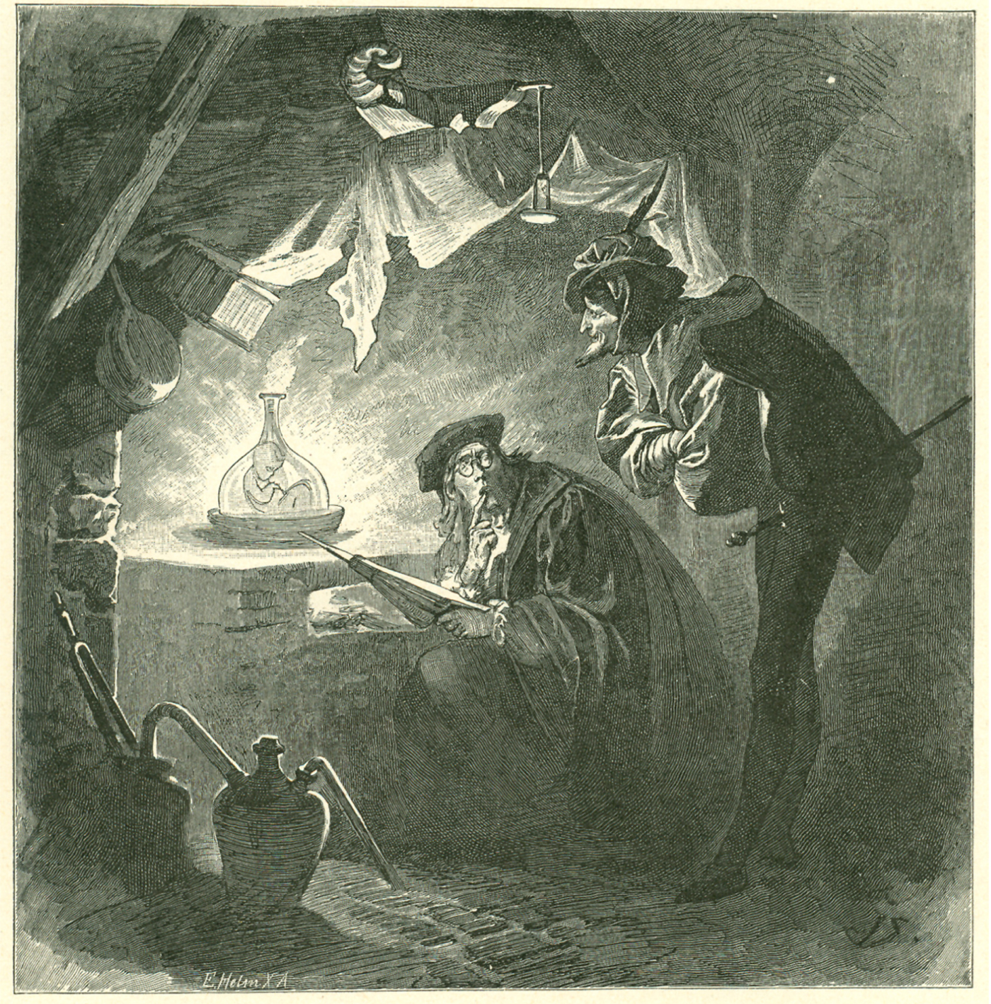
Fig. 1. The ability to create intelligent beings has long been a subject of endless fascination. With deep learning and the latest computers, we are coming close to achieving the dream of AI. (Image: ‘Homunculus in the vial’ by Franz Xaver Simm, 1899).
II. ORIGINS
John McCarthy is widely credited with coining the term ‘Artificial Intelligence’ in his 1955 proposal for the Dartmouth Workshop [Reference McCarthy, Minsky, Rochester and Shannon5], although the first artificial neuron described in 1943 [Reference McCulloch and Pitts6] and early work on speech recognition in 1952 [Reference Davis, Biddulph and Balashek7] predated the workshop. Work on computer vision started a decade later, circa 1966 [Reference Papert8], using vidisector video camera tubes. Despite the intense effort and funding poured into the development of AI, the problem proved to be challenging and for many years the advances made by researchers were unable to match the hype, resulting in periods of disillusionment and reduced funding known as the AI Winters.
Fast forward to the year 2017. AI-powered machines are outperforming human beings at diagnosing skin cancer [Reference Esteva9] and at the ancient game of Go [Reference Silver10]. Newer cars have enough autonomous navigation smarts, such that more adventurous drivers are letting go of their steering wheels while their cars cruise under computer control [11]. It is safe to say that the AI Winter is over. In fact, the recent explosion of advances in AI are changing the way many problems are solved to the extent that one can say the world is experiencing a Renaissance in AI.
In this paper, we take a look at the inner working of the representative deep neural network (DNN) architectures and highlight a number of recent advancements, and conclude with a discussion of open challenges and opportunities.
III. NEURAL NETWORKS AND DEEP LEARNING
In the year 2012, an artificial neural network (ANN) AlexNet [Reference Krizhevsky, Sutskever and Hinton12], named after its creator Alex Krizhevsky, beat all competitors by a large margin in the IMAGENET [Reference Russakovsky13] visual object recognition competition. Remarkably, it was the only entry employing an ANN that year, and in subsequent years virtually all submissions were ANN-based. A few years later in 2015, ANN-based solutions surpassed human performance in visual object recognition. AlexNet is without a doubt the landmark event that ignited the AI Renaissance and may be considered the first time that the three main ingredients of modern Deep Learning [Reference Goodfellow, Bengio and Courville14] came together: a massive training data set that was the IMAGENET training set, a software framework for training which took advantage of graphics processing units (GPUs) for hardware acceleration, and a deep convolutional neural network design.
A) Artificial neurons
An artificial neuron generally performs the following computation:
 $$y = A\left(\sum_{i} w_ix_i + b\right)$$
where y is the output, x i are the inputs to the neuron, w i are the weights applied to each input, b is a bias term, and A() is a non-linear activation function. In the earliest form, the inputs and outputs are binary [Reference McCulloch and Pitts6], with a step function for activation. The Perceptron [Reference Rosenblatt15] accepted continuous inputs and its learning algorithm guarantees convergence on linearly separable data sets. By constructing multiple layers of perceptrons where the outputs of one layer is input to all perceptron units in the next layer, such a feed forward neural network can learn more complex mappings.
B) Convolutional neural networks (CNN): AlexNet and VGGNet
While early ANNs are attempts at approximating biological neural nets, they were primarily implemented on digital computers, and algorithmic techniques which were able to execute efficiently on digital computers started inspiring new neural network designs. CNNs [Reference LeCun and Touretzky16] are one such class of network architectures. Drawing upon advances in image and signal processing, CNNs introduce layers where neurons have a limited receptive field (the kernel) and the weights are shared across a set of neurons that collectively compute a sliding window operation across the input layer (Fig. 2). At the i-th row and j-th column of the two-dimensional (2D) input field, the output of the corresponding neuron is
 $$S(i,j) = \sum_{m}\sum_{n} I(i-m,j-n)K(m,n)$$
where I is the input layer and K is the m×n kernel. In this case, the number of weights for this convolutional neuron is m×n, and for an input layer of size w×h, it computes an output feature map of about the same size. If a layer has c convolutional neurons, then it generates a c-channel output feature map. Additional parameters such as padding (for where the sliding window starts and ends at the input layer boundaries) and stride (the step size at which the sliding window moves across the input layer) can be changed to configure the output layer size. CNNs bring a number of key benefits:
(i) Size. Compared with a fully-connected multi-layer perceptron, where the number of weights in a network is the product of the input and output sizes, the number of weights for a convolutional neuron is determined by the size of the kernel. For example, a 1000-input, 1000-output layer would require 1 000 000 weights while a convolutional layer would just require m×n weights for each kernel. If a layer specifies 128 3×3 convolutional kernels, the number of weights is 1152. As a result, CNNs with similarly sized layers typically require orders of magnitude less space for storage.
(ii) Faster Execution. As a result of the smaller network size, CNNs can run faster on digital computers by taking advantage of faster memories higher up the hierarchy. For example, when computing a convolutional layer, weights which are heavily reused can be placed in high-speed cache memory. Since fast memory tends to be smaller than slow memory, smaller sized networks are better able to fit.
(iii) Training Speed. During the training of DNN, often parallel computation is utilized to increase throughput and decrease training time. The most commonly used data parallelism has multiple copies of the same network evaluated on a number of different processors, which can be on the same machine or distributed across multiple machines. In each cycle the processors need to synchronize their networks, and smaller networks can be transmitted faster, reducing the amount of processor idle time.
(iV) Flexibility. Since the output of each convolutional layer is generated in a sliding window fashion, the sizes of the layer input and output can be changed while keeping the layer weights constant. This means that if a neural network is fully convolutional, it can take inputs of arbitrary sizes during and after training.
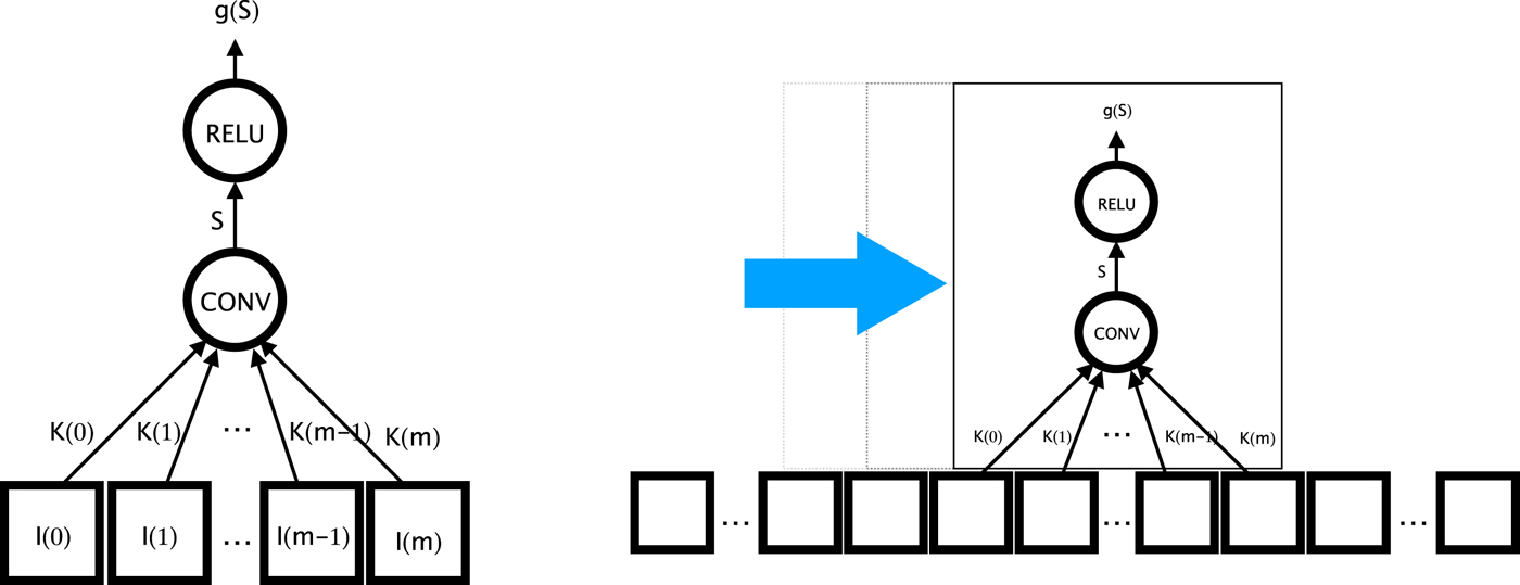
Fig. 2. A Convolution layer uses a shared set of weights for a set of neurons, effectively applying the same neuron across the input in a sliding window fashion.
In AlexNet, two different convolutional filter sizes were used: 11×11 and 3×3. CNN architecture is refined in VGGNet [Reference Simonyan and Zisserman17] to use only 3×3 filters. The 3×3 kernel is the smallest possible kernel with a sense of up/down/left/right/center. Using a smaller, standard-sized kernel brings more of the aforementioned computational benefits. To account for the loss in receptive field size going from 11×11 to 3×3, the designers of VGGNet increased the number of convolutional layers, effectively creating a vertical stack of convolutional layers, similar to how the different levels in a laplacian pyramid [Reference Burt and Adelson18] correspond to increasing large receptive fields. Fig. 3 shows the overall architecture for the VGG-19 network. As shown in the figure, it uses only five different kinds of layers: convolutional, rectified linear activation unit (ReLU), max-pooling, fully connected, and softmax. For completeness, we briefly review the layers used in the 19-layer VGGNet.

Fig. 3. The VGG-19 network [Reference Simonyan and Zisserman17], which uses only five types of layers. All convolution layers use 3×3 kernels and all max pool layers use 2×2 kernels. 19 counts only the convolution and fully connected layers. Due to the presence of fully connected layers, VGG-19 is not fully convolutional and therefore, will only be able to accept 224×224×3 inputs without retraining.
C) ReLU activation
We saw that early artificial neurons used non-linear activation like the step function. The most widely used activation function today is the ReLU:
 $$g(z) = max \{0,z\}$$
[Reference Krizhevsky, Sutskever and Hinton12] demonstrated that CNNs with ReLUs converge several times faster than an equivalent networks with tanh neurons. Parametric ReLU (PReLU) is a variant allows a non-zero response for negative input:
 $$g(z) = max \{0,z\} - \alpha\,max\{0,-z\}$$
D) Max pooling-layers
The max-pooling layers apply a sliding window over the input, similar to convolution layers, except each neuron outputs the maximum value in each respective window.
 $$MaxPool (i,j) = MAX_{\forall m,n} I(i-m,j-n)$$
Intuitively, max-pooling layers introduce spatial translation invariance to the network. Also similar to convolution layers, max pooling at multiple levels in a deep network introduce increasing amounts of translation invariance.
E) Fully connected layers
Fully connected layers consist of perceptron-like neurons that have real-valued inputs and output, where each neuron's input is connected to all elements of the previous layer. These are often the layers in a deep neural net with the largest amount of weights. For example, in the VGG-19 network, there are 4096 × 4096 = over 16 million weights just between the first two fully connected layers.
The last fully connected layer in VGG-19 has 1000 neurons, corresponding to the 1000 object classes to be recognized in the IMAGENET challenge. The input to the last fully connected layer can thus be considered a 4096-element feature vector that encodes information needed to recognize objects and often can serve as a rich abstract descriptor useful in many tasks.
F) Softmax
If the output from the final 1000-neuron fully connected layer in VGG-19 can be considered a set of confidence values for each object class given the input image, the softmax layer which computes
 $${softmax}(z_i)=\displaystyle{{exp}(z_i) \over \sum_{j}{exp}(z_j)}$$
where z i is the output from a neuron in the previous layer. Softmax serves to apply ‘contrast enhancement’ and normalization to ensure the output is a probability distribution that sums to 1.
G) Training a DNN
After the network architecture is defined, it needs to be trained in order to assign values to the tunable parameters in the layers. Networks can easily have tens of millions of parameters that need to be individually tuned in order to produce optimal results for each data set, which in turn can consist of millions of images, hundreds of hours of audio recordings, for example. The most commonly used technique for tuning these parameters to fit labeled data sets, or training neural networks, is the Stochastic Gradient Descent (SGD) method.
Figure 4 shows the steps in SGD. In each iteration, a set of training samples is randomly selected along with the labels for each sample that correspond to the correct answer that the neural network should produce. For each (data, label) pair we need to find the direction in which to modify each parameter so that the error between the network output and label is minimized. This can be done by differentiating the error or loss function with respect to the weights, to obtain the error gradient
 $$\nabla_{w_{t}}J = \displaystyle{\partial J_t \over \partial w_t},$$
where J represents the error. The weights can then be updated using
 $$w^{\prime} = w - \eta \nabla_{w}J$$
where η>0 is an appropriate learning rate, that controls the amount of adjustment, as we adjust the weights along the direction of greatest reduction in error. The gradient can be computed using the Backpropagation [Reference Rumelhart, Hinton and Williams19] algorithm, which consists of two steps in each iteration:
(i) Forward Propagation (Fig. 4(2)) Where the output of each layer i is computed using output from previous layers and the current set of weights.
 $$y_i = f_i(w_i, y_{i-1})$$
(ii) Backward Propagation (Fig. 4(5)) The error or loss function J is computed from the output from the final layer and the corresponding label or ground truth for the training data. Since J is computed from a function of w N, the weights from the final layer N, the gradient for updating w N can be computed directly:
and gradients for weights w i in each layer i can be computed recursively using the chain rule:$$\nabla_{w_N}J = \displaystyle{\partial J \over \partial w_N}$$$$\nabla_{w_i}J = \displaystyle{\partial J \over \partial w_{i+1}}\displaystyle{\partial w_{i+1} \over \partial w_i} = \nabla_{w_{i+1}}J \displaystyle{\partial w_{i+1} \over \partial w_i}$$


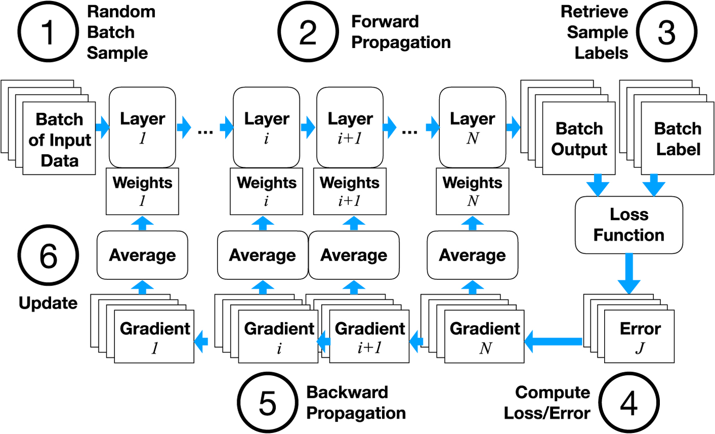
Fig. 4. How to train a DNN with SGD and backpropagation.
H) Vanishing gradients and residual connections
While the basic idea of backpropagation has remained unchanged for several decades, it was not until recently that researchers have successfully trained truly DNN with many layers. Aside from the availability of powerful computers, techniques have also been proposed that address the so-called vanishing or exploding gradient problems, where the gradients computed by backpropagation become very small or very large, causing convergence to stall or to introduce unstably large swings in the update steps. Solutions proposed to address this challenge include batch normalization [Reference Ioffe and Szegedy20] which reduces covariate shifts in intermediate layer outputs and the use of ReLU non-linear activation, which does not saturate with large input values (unlike for example, the sigmoid activation function). The most dramatic improvement perhaps came with the introduction of residual connections in ResNet [Reference He, Zhang, Ren and Sun21]. Residual connections, as illustrated in Fig. 5, are the links that skip pass a number of layers such that if the original block of layers is represented by
 $$y = f(x)$$
then the residual connection turns the output into
 $$y = f(x) + x$$
which of course requires the input x and the output f(x) to have the same dimensions in order that a tensor addition is possible. In [Reference He, Zhang, Ren and Sun21], it was reported that very DNN with 1000 layers was successfully trained. The winner of the ILSVRC 2015 classification task was a 152 layer network. Remarkably, even though it was 8x deeper than VGG nets the computational complexity is lower. Densenet [Reference Huang, Liu, van der Maaten and Weinberger22] (Fig. 5) adds even more residual connections that skip through more blocks. Intuitively, the main benefit of residual connections can be thought of as allowing the error signal to flow through more layers during backward propagation.
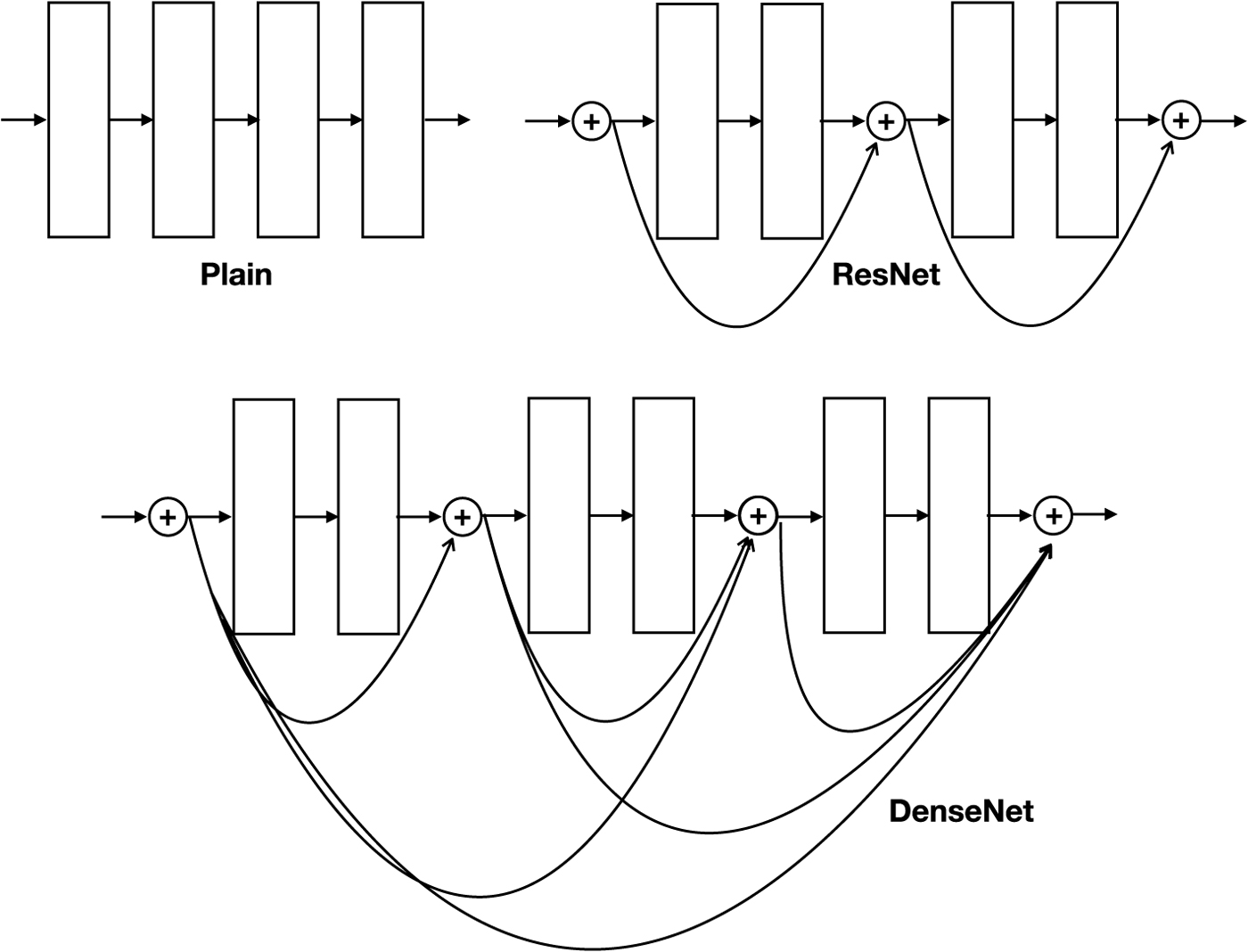
Fig. 5. Direct connections enables training of deeper models.
I) Recurrent neural networks
Many real-world applications involve signals that are temporal in nature – for example the acoustic speech signal varies spectrally over time; in natural language, words form sentences, and their ordering can drastically alter meaning to convey different semantics. Some of these types of dependencies can occur over very long spans of time [Reference Lau, Rosenfeld and Roukos23]. By analogy – IIR filters can more compactly describe filter responses that would otherwise take thousands of samples in the impulse response to effectively model [Reference Oppenheim and Schafer24] – thus so-called recurrent neural networks can provide far greater modeling power compared with purely feed-forward networks, as they are able to capture information and learn from a much longer context [Reference Lipton25,Reference Bengio26].
Figure 6 shows how recurrent links work for a single neuron. A recurrent network simply has links such as to cause the network graph to become cyclic. While in the past, other networks with more ad-hoc or amorphous topologies have been proposed, most recent RNN incarnations do not really have recurrent links across layers. Many algorithms have been proposed for training RNNs, the most popular might be backpropagation in time (BPTT) [Reference Rumelhart, Hinton, Williams, Rumelhart and McClelland27], which ‘unrolls’ recurrent links so that the network can be approximated by a larger, fully feedforward network. Thereafter, the network can be trained using variants of SGD – this is illustrated in Fig. 7. The difficulty with training such networks is, similar to the problem of depth, error signals are prone to either blow up or vanish exponentially as they propagate backwards through time. Consequently, the updated gradient explode or vanish, leading to unstable training and the inability of the recurrent networks to model long-span dependencies [Reference Bengio, SImard and Frasconi28].

Fig. 6. Recurrent connnections in a single neuron recurrent neural network (from [Reference Lipton25]).
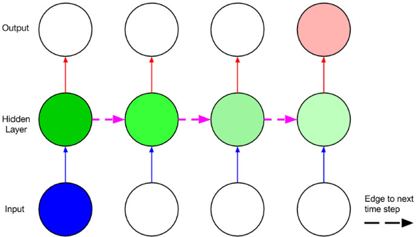
Fig. 7. Unrolling recurrent links through time with the BPTT algorithm (from [Reference Lipton25]).
Long short-term memory (LSTM) [Reference Hochreiter and Schmidhuber29] cells were proposed to tackle the vanishing gradient problem in BPTT, and they work by enforcing constant error flow during backpropagation. This is done by introducing gating mechanisms around a memory element that tracks the cell's inner state – an input-gate controls the amount of information flow to the memory cell, an output-gate controls the information flow from the memory cell to the next layer, and a forget gate controls information flow between cell memory from the previous to the current time state. This is illustrated in Fig. 8. Common variants of the LSTM cell may include using different combinations of either including or excluding the input, output, and forget gates or introducing so-called peephole connections which are, for all practical purposes, residual connections that bypass the gating mechanism [Reference Greff, Srivastava, Koutník, Steunebrink and Schmidhuber30].
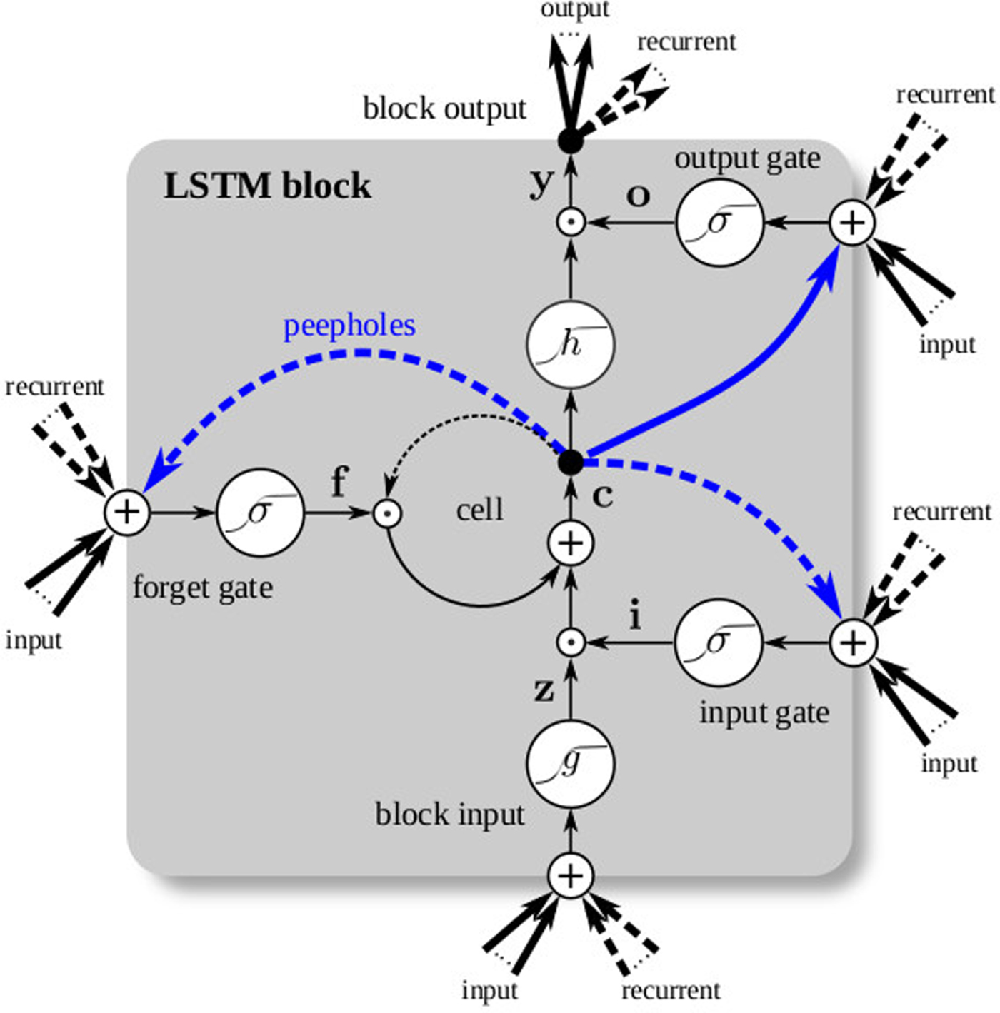
Fig. 8. An LSTM cell helps to enforce constant error flow in BPTT. (from [Reference Greff, Srivastava, Koutník, Steunebrink and Schmidhuber30]).
A further refinement of LSTMs integrates information from past and previous time frames by stacking a backward LSTM layer on top of a forward LSTM layer. In this case, the backward LSTM is identical to the usual, forward LSTM, except that recurrent links use inputs from frames in the future as opposed from frames in the past. Today, bi-directional LSTMs are a staple [Reference Amodei31,Reference Graves32] of acoustic modeling. They have been used in conjunction with the connectionist temporal classification (CTC) loss function to obtain the best known speech recognition results on continuous telephony conversational speech [Reference Xiong33]. Recent work has also shown that the [Reference Wang, Chung and Lee34] forget gate activations in trained recurrent acoustic neural nets such as correlate very well with phoneme boundaries in speech activation – this validates many approaches to speech recognition and other sequence modeling problems which involve recurrent networks.
J) Hardware acceleration
Fast computers have always enabled new advances, although often not in the domain the computers were originally designed for. The same can be said of GPUs that are fueling most development in deep learning and AI. As name implies, Graphics Processing Units were originally designed for rendering 3D scenes consisting of large collections of texture-mapped triangles. As the sophistication of rendering pipelines grew, GPUs became increasingly programmable, with little programs called shaders that allowed highly customized effects in lighting, geometry, and rasterization. Researchers and engineers gradually started to use GPUs to accelerate non-graphics computation, giving rise to General-purpose GPU (GPGPU) techniques [Reference Pharr and Fernando35]. Early GPGPU programming essentially expressed algorithms in terms of Computer Graphics commands, which meant having to work within the limitations of an API that was not designed for general purpose computation. Eventually, compilers designed for expressing parallel computation on GPUs appeared [Reference Buck36], and evolved into widely-used libraries like CUDA [Reference Nickolls, Buck, Garland and Skadron37] and OpenCL [38]. Today GPUs are commonly used as SIMD parallel computers powering deep learning, cryptocurrencies, and molecular simulations.
Today another class of new computation devices and processing units is emerging: the AI accelerator. The best known example is Google's Tensor Processing Unit (TPU) [Reference Jouppi39], which was motivated by the realization that if all of their users started using voice recognition cloud services for 3 min a day, Google would have to double their data center capacity. The first version of the TPU is essentially designed to accelerate matrix multiply-add operations on matrices and tensors.
Figure 9 shows a taxonomy of computational hardware devices broadly grouped by power consumption (Horizontal axis) and raw computational ability (Vertical axis). The left-hand column represents the devices consuming hundreds of Watts, typically deployed in cloud data center servers and desktop computers. In the lower left-hand quadrant are the traditional CPUs that perform tens of billions of operations (Gigaops). GPUs sitting in the upper left-hand quadrant are equally, perhaps even more power hungry, but are capable of delivering computational power in the Teraops range. On the right-hand side we have the devices that consume less power, and are often used in battery-operated systems. In the lower right-hand quadrant are the energy efficient devices available today, typically in the form of Digital Signal Processors (DSPs). In each quadrant, we also listed a representative problem solved by computers in each class. CPUs which powered Deep Blue, were able to defeat Gary Kasparov, the world champion in International Chess, with 11 Gigaops. AlphaGo needed GPUs and TPUs to outplay Ke Jie, the world champion in Go, with an estimated 100 Teraops. DSPs consuming around 1W were able to bring to life an aerial drone that is able to respond to hand gesture commands and take selfies [Reference Michael40]. The upper right-hand quadrant is where AI accelerators will be, delivering 10 s of Teraops while consuming 10W or less. We believe these AI accelerators [Reference Lu41] (Fig. 11) will be instrumental in realizing self-driving cars and ushering in the age of Intelligent Internet of Things (I 2oT).
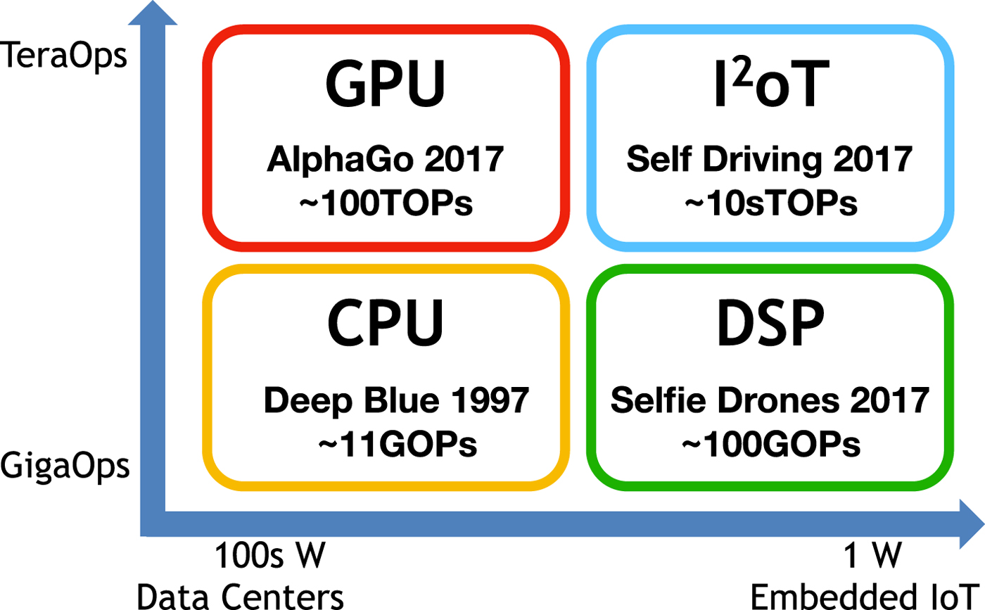
Fig. 9. A taxonomy of hardware platforms for AI.
IV. APPLICATIONS
With the recent advancements in deep learning and AI, many longstanding problems can now be solved reliably and are finally fit for deployment in real-world applications. These advances seem to reduce the many traditional AI problems into a matter of data collection and labeling - yet simply treating the neural network as a black box is not enough. For example, there may be several choices for the type of label or type of feature input to the network, or some underlying meaning to the semantic function of intermediate layers - this is better guided by some understanding of classical literature. We review a number of these representative examples of success in the AI Renaissance and point out where careful integration of classical ideas have considerably boosted performance or aided understanding.
A) Object recognition
Perhaps the best illustration of what deep neural nets can do is object recognition. As the central problem in the IMAGENET challenge [Reference Russakovsky13], it has inspired AlexNet [Reference Krizhevsky, Sutskever and Hinton12], the network that originally sparked the AI Renaissance, followed by VGG [Reference Simonyan and Zisserman17] and ResNet [Reference He, Zhang, Ren and Sun21], as the AI community converges around very DNN. Fig. 10 shows an object recognition demonstration powered by a VGG network running on NovuMind's AI Processor prototype.
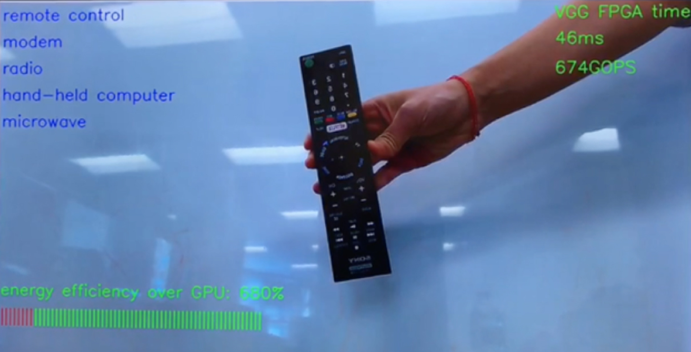
Fig. 10. Object recognition: A VGG network running on NovuMind's AI processor FPGA prototype performs real time object recognition. Upper left-hand corner lists the top-5 recognition results.
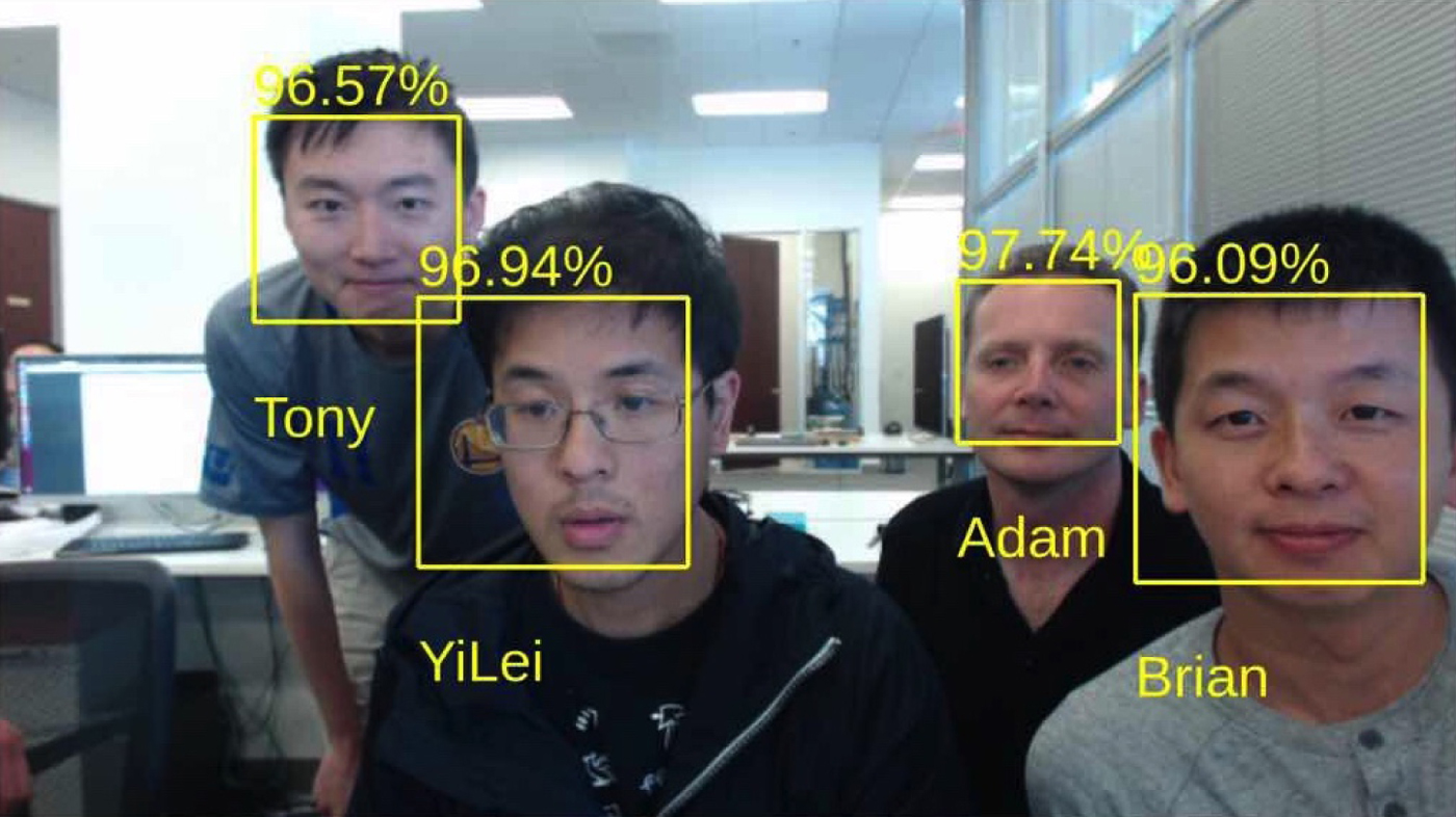
Fig. 11. Face recognition on NovuMind's AI processor FPGA prototype running in real time.
Networks trained to classify IMAGENET images often can also be used to provide the initial set of weights for networks that are meant for other purposes, and have been shown to converge faster than when initialized with random numbers.
Due to the comprehensiveness of the IMAGENET data set, neural networks trained with this data set to a high degree of accuracy on the object recognition task can be considered to have learned to extract features that are useful in other visual tasks. For example, if we look at the output of the second-to-last fully connected layer in the VGG network, it is an abstract descriptor for the input image and for example one way to determine if two images are similar would be to compute the VGG feature vector for both images and then finding the L 2 distance or dot product between the two vectors [Reference Rosenthal42].
B) Face recognition
One domain where the abstract feature vector approach has been successfully applied is face recognition [Reference Chen, Ranjan, Kumar, Chen, Patel and Chellappa43,Reference Schroff, Kalenichenko and Philbin44]. Given a large enough set of face images labeled with the identification of the people whose faces appear in the images, a neural network can be trained to extract a feature vector descriptor of faces, and classification algorithms can work with the vectors as points in a high-dimensional space. If the data set captured sufficient variations in pose, lighting, expression, etc., the resulting feature vector will accordingly be invariant to these factors to a large extent. Coupled with face detection capabilities, it is now possible to build face recognition systems that are capable of recognizing faces under fully unconstrained settings (Fig. 12), without the need of subjects to even be aware of the recognition system.
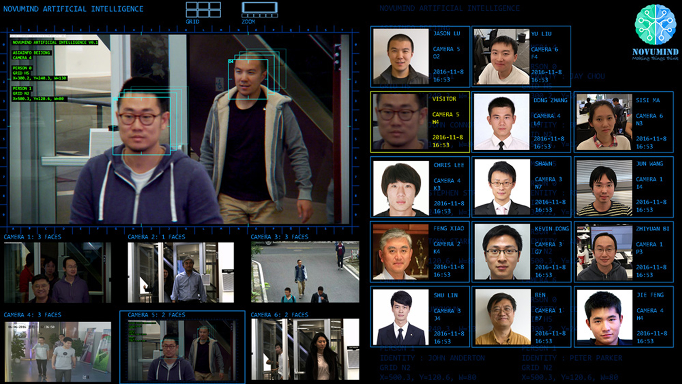
Fig. 12. NovuMind Unconstrained Face recognition system identifies employees and visitors in real time.
C) Object detection
If we think of object recognition neural networks as consisting of a deep convolutional feature extractor followed by a feature vector classifier, object detection can be performed by replacing the classifier by a stage that estimates the spatial bounding boxes of objects of different kinds in images [Reference Redmon and Farhadi45,Reference Ren, He, Girshick and Sun46]. Object detectors have many applications, including in autonomous driving (Fig. 13) and face detectors are integral parts of face recognition systems.
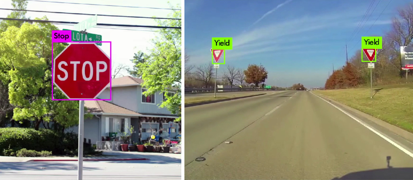
Fig. 13. Object detection with convolutional neural networks. A network trained to detect and recognize traffic signs may have applications in autonomous driving.
The ability to estimate body pose [Reference Cao, Simon, Wei and Sheikh47] directly from monocular images is also a dramatic example of success for DNN. Until recently, the only reliable way to track body pose was with depth cameras that employed structured light or time-of-flight sensors, which are limited mostly to indoors or short-range settings.
D) Semantic segmentation
Segmentation is another long-standing problem in computer vision that has been successfully addressed by DNN segmentation [Reference Girshick, Donahue, Darrell and Malik48], partly because the ability of DNN to recognize many different kinds of objects has made it tractable to pose the previously ill-posed ‘segmentation problem’ as that of labeling pixels corresponding to the physical objects in images. Since CNN feature maps tend to be much lower in spatial resolution, deconvolution or transposed convolution layers are used to generate higher resolution segmentation maps.
Instance aware segmentation [Reference Li, Qi, Dai, Ji and Wei49] is a further refinement of the problem where multiple occurrences of the same type of object are separately segmented. One way to achieve this is essentially to perform object detection, and then segment within the bounding box of each detected object [Reference He, Gkioxari, Dollár and Girshick50]. Segmentation for specific purposes, like portraits [Reference Shen51] have also been demonstrated.
E) Colorization
The ability to label each pixel in an image semantically by its physical object class has also made it possible to design deep networks that perform colorization [Reference Zhang, Isola and Efros52], the problem of generating a plausible color image from a monochrome input image. Fig. 14 shows an example.
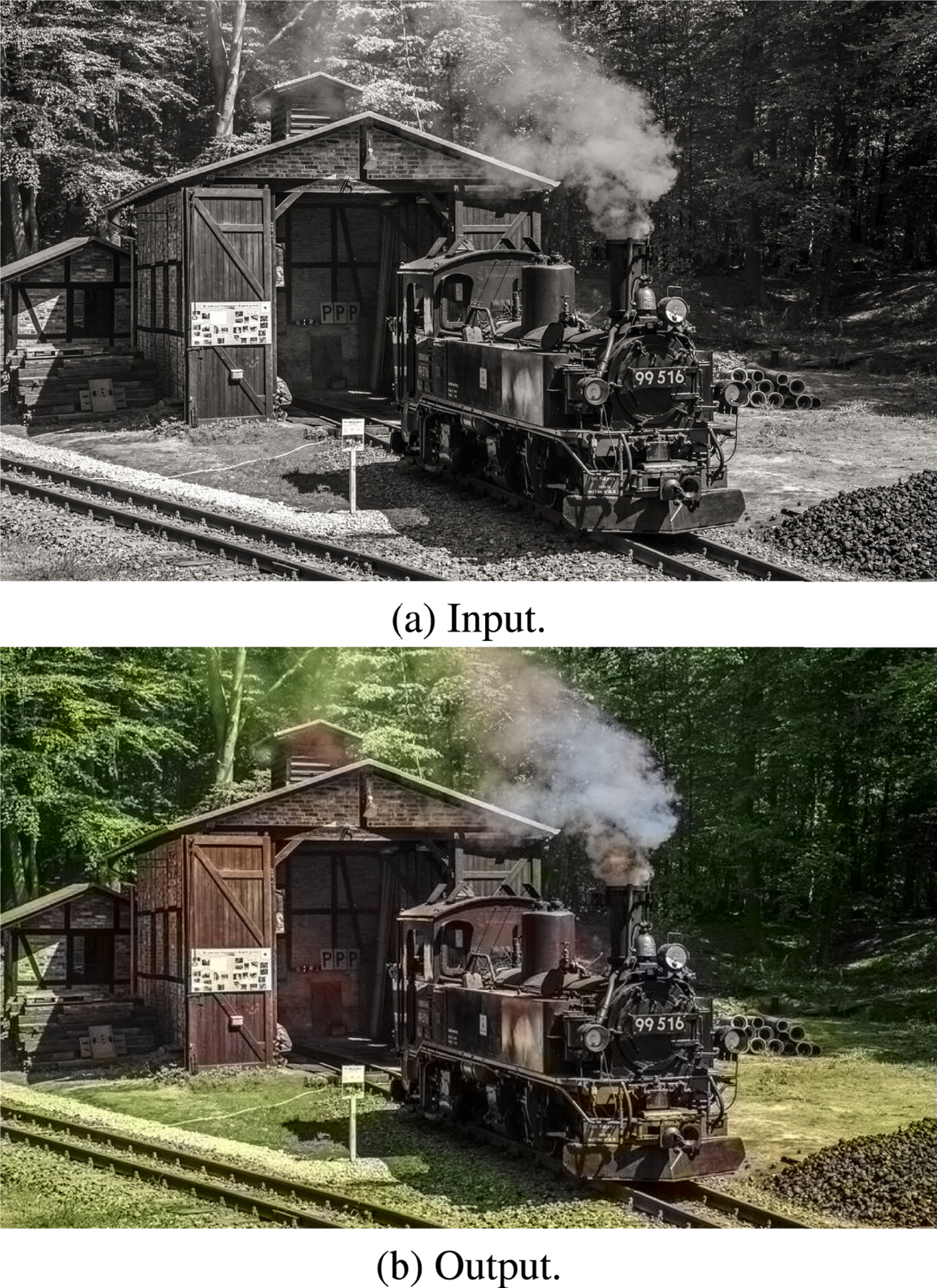
Fig. 14. Automatic colorization with a DNN [52]. (a) Input monochrome image. (b) Output colorized image.
F) 3D depth
If a DNN can estimate the RGB color for each pixel in an image, can it also estimate depth? Remarkably, it has also been demonstrated that it is possible to generate a reasonable depth map from a single monocular image [Reference Laina, Rupprecht, Belagiannis, Tombari and Navab53] (Fig. 15). While the depth map generated is not as good as state of the art 3D reconstruction methods, it can already be useful for human–computer interactions where having absolute accurate depth is not critical, and can be refined by image fusion [Reference Yang, Tan, Culbertson and Apostolopoulos54,Reference Yang55]. The monocular depth estimation algorithm has also been shown to be a good initial estimate in a SLAM algorithm [Reference Tateno, Tombari, Laina and Navab56], helping to overcome challenges where scenes have large featureless regions like interior walls in many office buildings.
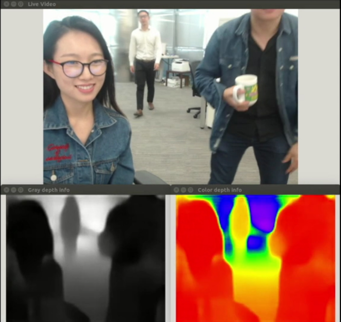
Fig. 15. Monocular depth estimation with a DNN. (Top) Input RGB image. (Bottom) Output depth map in grayscale and pseudo color.
G) Image synthesis
In addition to estimating quantities and recognizing object classes, modern neural networks can also be designed and trained to output images that are meant for human viewing. A very popular application is stylization, where an input image is re-rendered to take on distinctive characteristics of another [Reference Gatys, Ecker and Bethge57,Reference Johnson, Alahi and Fei-Fei58]. For example, one can re-render pictures of friends, city scenes, or the house cat to look like paintings by Vincent van Gogh, Piet Mondrian, or Pablo Picasso.
An interesting problem in training this kind of neural network is how the error signals can be generated during backpropagation: for a classification or estimation problem it is straightforward for a human being to provide the right answer, but how can labels for abstract or complex criteria like whether an image looks like a van Gogh painting be generated? One way to do it is with another neural network! With Generative Adversarial Networks [Reference Goodfellow59,Reference Arjovsky, Chintala and Bottou60], in the training stage, a discriminator network is appended to the end of the generator network one is training. The discriminator network takes as input the result of the generator network, and decides whether the input satisfies the criterion, for example whether the input image is a Picasso painting or not. This discriminator network essentially turns the complex criterion into a binary classification problem, and can be trained with human-labeled data sets (say of Picasso paintings labeled 1 and natural images labeled 0). Once the generator network is trained to output images that consistently passes the discriminator's classifier, the discriminator network can be discarded.
H) Reinforcement learning and tracking
Deep reinforcement learning is a method that trains a DNN to learn to predict the next action for a system or algorithm to take in order to achieve a longer-term goal. It was most famously used to train the AlphaGo [Reference Silver10] program that bested human world champions at the ancient board game. In the Go example, each game has a sequence of moves by both players leading up to the final outcome. How good each move is for each player can be assigned based on the final outcome, and the goodness for each step throughout the game can be discounted based on how close to the end of the game the move is. This way, the neural network can be thought of as learning a strategy that incorporates considerations for subsequent moves in addition to the immediate configuration.
This approach of learning a strategy for taking actions has also been applied to solving the problem of tracking [Reference Yun, Choi, Yoo, Yun and Choi61], where the decision for where to move the bounding box for the object being tracked is formulated as a strategy to be learned with reinforcement learning.
Reinforcement learning can also be used in other types of problems involving turn-taking situations – such as in generating dialogue for chatbots from the previous conversation turns [Reference Li, Monroe, Ritter, Jurafsky, Galley and Gao62]. This can be effective in open-dialogue scenarios like conversational chatbots, in which there may not necessarily be a task that needs be completed through the dialogue interaction.
I) Aerial drone control
Aerial drones are set to change the way packages (including emergency medical supplies, rescue equipment, or postal parcels) are being delivered, but indoor navigation and obstacle avoidance especially in natural environments remain a challenge. Flight control systems that incorporate DNN that help drones stay on forest trails where there are no lane markings have been demonstrated [Reference Smolyanskiy, Kamenev, Smith and Birchfield63] and hold the promise to enable drones to reach places that are not possible to reach today.
J) Crossing domains
One of the most interesting class of neural network advances recently have been algorithms that cross different domains. Perhaps the most impressive results are the captioning algorithms: generating a sentence that describes the content of images or video [Reference Mao, Jonathan, Toshev, Camburu, Yuille and Murphy64,Reference Xu, Bach and Blei65], and also algorithms that take a sentence and synthesize a photorealistic image that fits the textual description [Reference Zhang66]. Extrapolating to the far future, one can imagine systems where the scripts of movies or TV programs are transmitted over the air, and the actual audio-visual content is synthesized from the textual script, customized for each household depending on who is viewing the program.
K) Speech recognition
Similar to computer vision, deep learning has impacted speech and language research in a big way. Up till recently, accurate, human-level speech recognition performance in all manners of adverse conditions was considered to be an unattainable holy grail, with large gaps in performance identified at the acoustic level [Reference Lippman67,Reference Juneja68]. Today, the gap is closing for some types of speech signals, for instance in relatively clean, telephony conversations on provided topics (i.e. switchboard) [Reference Xiong69].
Neural networks for acoustic modeling were proposed as early as 1989 in the form of time-delay neural networks (TDNN [Reference Waibel, Hanazawa, Hinton, Shikano and Lang70]. It is, however, only recently that we have seen good successes with these methods by using larger datasets, more compute and better training algorithms. Dong et al. [Reference Dahl, Yu, Deng and Acero71], replaced the posterior probabilty estimation component, formerly powered by Gaussian Mixture Models (GMMs) with feed-forward, fully connected DNN, and immediately saw a 15 to 20% relative improvement in accuracy. Some recent extensions of this used a combinations of different types of neural networks - for instance a sequence of Convolutional, LSTM, and feed forward Deep neural network layers (CLDNN) [Reference Sainath, Vinyals, Senior and Sak72], currently give the best performance all around. Neural networks continue to proliferate in all areas of speech and language processing, including speech recognition [Reference Dahl, Yu, Deng and Acero71], synthesis [Reference Wu, Watts and King73,Reference van den Oord74], speech enhancement and separation [Reference Huang, Kim, Hasegawa-Johnson and Smaragdis75], machine translation [Reference Vaswani76], and dialogue [Reference Vinyals and Le77].
The classical ‘beads on a string’ model [Reference Ostendorf78] of speech, in which we assume that spoken utterances can be generated by a quasi-stationary stochastic process, naturally gave rise to the use of Hidden Markov Models [Reference Baker79,Reference Lee, Waibel and Lee80]. This approach is frame-synchronous and furthermore decouples the speech recognition into two sub-problems, one of classifying an incoming speech frame to a correct sound class (the acoustic model), and modeling of transitions from one sound to another as well as the likelihood of word sequences in the language (the language model). This framework has largely persisted as the dominant approach until recently – however, we are starting to see novel deep-learning architectures leapfrog and take over the traditional approach. Several researchers have proposed point-process models [Reference Niyogi and Jensen81], articulatory models [Reference Zweig82,Reference Lee83], and landmark-based speech recognition [Reference Hasegawa-Johnson84]. These methods consider speech as a sequence of discrete events that do not necessarily occur at regular time intervals – that is we now move away from a frame synchronous approach to an acoustic event based approach. These ideas have a stronger foundation from speech science – it would seem plausible that one does not need to attend to every part of the speech signal with equal significance, but rather just the key events – such as release burst in plosives – in order to correctly identify the uttered speech sound. CTC [Reference Graves32] and its loss function is often used with recurrent neural nets. In the CTC approach, a neural network tries to classify speech sounds at each audio frame, but permit a ‘blank’ symbol to be emitted at frames which may not significantly contribute to the speech. In a sense, this is closer to an event detection sort of a framework, and can be thought of as breaking away from the frame-synchronous approach. The CTC loss function, optimizes the network to minimize the Levensthein (minimum edit) distance between classifier output sequence and the target transcription sequence. The CTC loss function itself is a direct result of applying a fundamental understanding of how Baum–Welch (i.e. how classical speech recognition) works, to improve the training process for speech/acoustic neural networks. The later work, demonstrated that the CTC loss function could be used with character sequences as targets, paving the way for so-called end-to-end speech recognition systems [Reference Amodei31,Reference Yajie Miao and Gowayyed85], which, unlike traditional approaches, require almost no additional linguistic knowledge or resources beyond transcribed audio and language. This approach almost completely cuts out the involvement of linguistics in modern speech recognition training at the expense of requiring a few orders of magnitude more data in order to achieve parity in performance. This is a clear indication that careful application of our understanding of linguistics and neuroscience, can still have tremendous impact, and it is possible that we have yet to fully realize how much further we can push deep learning by appropriately incorporating domain knowledge.
Even newer paradigms such as sequence-to-sequence learning [Reference Chan, Jaitly, Le and Vinyals86], completely forgo both frame-synchronous and event-detection frameworks and simply treat the speech recognition problem as a translation problem between audio and actual text. Here, a neural network comprises an encoder sub-network that listens and encodes the audio into an intermediate format, an interemediary network that attends to what it thinks are important parts of the encoding, and a decoder that decodes by spell-ing it back into text. This so-called listen, attend, and spell (LAS) model uses unique types of DNN to perform each task. The authors were able to attain a word error rate of 10.3% on a voice search task using a language model, not too far from the best CLDNN systems at 8.0%.
L) Speaker adaptation and normalization
Many interesting developments in speech recognition partially result from ‘porting’ concepts from earlier frameworks into deep learning. For example, discriminative training for acoustic models, using either the minimum phone error (MPE) or maximum mutual information (MMI) criterion is one example [Reference Povey and Woodland87]. The analogy for this in the hybrid-DNN framework would be state-level Minimum Bayes’ Risk (s-MBR) [Reference Vesely, Ghoshal, Burget and Povey88], in which the neural network is trained with a loss function that causes the correct frame-wise state sequence to stand out over a competing background of alternatives. Other classical methods have improved speech recognition, but for which there is no strong analogy in neural network terms. Speaker adaptation, which deals with rapidly adjusting a speaker independent acoustic model is an example. While techniques such as maximum likelihood linear regression (MLLR) [Reference Gales and Woodland89], maximum a priori probability (MAP) adaptation [Reference Gauvain and Lee90], or eigenvoice [Reference Roland Kuhn, Junqua and Niedzielski91] have been shown to be very effective, there may not be clear, fully neural network based analogues. For instance, techniques such Learning Hidden Unit Contributions (LHUC) [Reference Swietojanski and Renals92] work directly on the weight matrices of the neural networks instead of actually using a network layer to implement the ideas. However, other methods such as i-vector-based adaptation [Reference Saon, Soltau, Nahamoo and Picheny93], summarizing speaker neural networks [Reference Vesely, Watanabe, Zmolikova, Karafiat, Burbget and Cernocky94] come close.
Another example is speaker adaptive training [Reference Anastasakos, McDonough, Schwartz and Makhoul95] which is a paradigm that explicitly normalizes speaker variability during the training process. The subspace GMM [Reference Povey96] methods which try to explicitly factorize variabilities into separate vectors, can be thought of as an extension of this. Consequently, there is no real analogue for these, some training approaches will in fact use feature-MLLR [Reference Povey and Saon97], a popular classical speaker normalization method to produce features as inputs to the neural network. These ideas actually run in direct opposition to current deep learning paradigms, which prefer to implicitly handle variability through aggressive data augmentation and expansion [Reference Cui, Goel and Kingsbury98], rather than explicitly handling variability. It is clear that directly applying analogous concepts from earlier GMM systems to DNN have yielded some simple but important improvements to the core technology. Analogies for these concepts to end to end systems or sequence approaches are only starting to be explored at this point.
M) Speech signal processing
Even signal-processing in the front-end is not spared from this relentless march of deep learning. In [Reference Verma and Schafer99], it was demonstrated that a neural network can be trained to detect pitch directly from raw audio samples. The best performing network uses two layers – since the input to each neuron in the first layer can be thought of as a direct implementation of an FIR filter, taking the Fourier transform of the weights gives us a frequency response map, and by sorting the neurons in the first layer according to the peak frequency response, it appears that the network is effectively tuning in to various frequency peaks according to a frequency scale. After sorting the order of neurons in the first layer by their tuned peak frequency response, analysis of the second layer suggests that a set of comb-like filter structures is being learnt – this demonstrates the ability of the network to converge to a structure almost identical to traditional pitch tracking signal processing methods. In [Reference Sainath, Weiss, Senior, Wilson and Vinyals100], the authors showed that a frontend could be learnt that at least matched the performance of more traditional signal-processing feature extractors such as Mel-Frequency spectra. Furthermore, they demonstrated that the neural network provided complementary information to the spectral features. Other examples of deep learning in the frontend include [Reference Schrank, Pfeifenberger, Zöhrer, Stahl, Mowlaee and Pernkopf101], which use DNN to perform multichannel beamforming. Neural networks can now solve some speech enhancement problems as well as classical approaches, such as learning of time-frequency masks in order to do speech separation [Reference Huang, Kim, Hasegawa-Johnson and Smaragdis75], or dereverberation [Reference Xiao102]. The attractiveness of deep learning here is that the computation becomes very simple, since now every stage of processing can be done by neural networks. Even so, it still seems likely that classical methods still have much to contribute in terms of guiding our search for better ANN-based techniques and topologies.
N) Language modeling
Language modeling can be naively thought of as building a model to predict the next word given the history of past words in a sentence. It has key application in many areas of speech and language processing, including speech recognition [Reference Biadsy, Ghodsi and Caseiro103], machine translation [Reference Luonog, Kayser and Manning104], and natural language understanding. Despite the many possible words choices available in a language, say English, the next word choice when predicting words from a sentence fragment, is actually quite limited once we consider previous context. Perplexity, given by
 $$PPL \triangleq 2^{H(X)} = 2^{-\sum_X p(X) log_2 p(X) },$$
measures this directly. Here X is a discrete random variable that can assume one out of many possible words in a vocabulary V, and we can treat the production of words in a sentence as a random process. Often-times perplexity of a language model can be estimated by first computing the cross-entropy Ĥ(X) of the language model over a held out test data set.
Recent advances using neural networks have allowed very low-perplexity language models to be built. Both LSTMs and GRUs have been shown to model language very effectively. This is evidenced by recent works with the Google Billion Word Benchmark, in which a combination of RNN and Maximum Entropy (MaxEnt) models – key results are reproduced in Fig. 16 – have demonstrated a dramatic reduction in word perplexity over n-gram approaches [Reference Chelba105]. The reduction in perplexity from over 237 (K-N smoothed n-grams) to roughly 50, should really be considered an improvement of several orders of magnitude considering the exponentiation in the perplexity equation, and that is made possible by advances in deep recurrent neural networks.

Fig. 16. Comparison of n-gram and RNN-based language models.[Reference Chelba105].
Large neural network language models still remain very difficult to train – the best models have many more parameters compared with n-gram models and thus necessarily require larger datasets for training. Some advances seek to reduce the number of parameters required, either through combining character-based RNNs [Reference Jozefowicz, Vinyals, Schuster, Shazeer and Wu106,Reference Kim, Jernite, Sontag and Rush107], or through factorization of the weight matrices of the model [Reference Kuchaiev and Ginsburg108]. Such models have reportedly reached perplexity of 23.7 on the same billion-word benchmark set. RNNs also have the drawback that the recurrent links create very tight temporal dependencies, and thus make them difficult to parallelize effectively on commodity deep learning hardware (i.e. GPUs). An alternative might be to use deep convolutional networks – gated-CNNs have been shown to be able to mimic very long span n-gram modeling (i.e. 13), that tremendously lowers perplexity [Reference Dauphin, Fan, Auli and Grangier109]. Typically, n-grams language models require a lot memory to train and minimize, this gives more memory efficient way of building language models.
Despite these advances, ensemble methods fusing contributions from both RNN and n-gram models still give tremendous improvement over purely neural models – one of the best ensemble methods reported to date fuse skip n-grams with RNNs [Reference Shazeer, Pelemans and Chelba110]. This is evidence that despite the tremendous improvements to language modeling made possible via deep learning, we neither forget nor underestimate the remaining potential for classical methods to contribute to the field. Perhaps, in this new era of artificial intelligence, in equalizing the playing field by providing accessibility to simple-to-use deep learning frameworks, domain knowledge is more valuable than ever.
O) Speech synthesis
Speech synthesis deals with the problem of vocalizing text. Figure 17 shows an overview for a speech synthesis system. The frontend preprocesses raw text to generate linguistic features which drive a backend waveform generator.
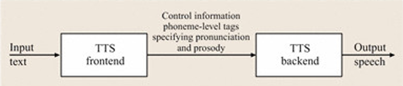
Fig. 17. Block diagram for text to speech synthesis systems. (from [Reference Schroeter111]).
Conventional methods prior to deep learning can be categorized into a main few – articulatory synthesis based on our understanding of human speech production [Reference Ling, Richmond and Yamagishi112], formant synthesis [Reference Klatt113] based on the source-filter model of speech production, concatenative synthesis using unit selection [Reference Hunt and Black114], and recently statistical parametric speech synthesis [Reference Black, Zen and Tokuda115]. Up till recent times, unit selection has dominated as the most practical method for natural sounding synthesis – but the discovery of wavenets [Reference van den Oord, Deileman, Zen, Simonyan, Vinyals, Graves, Kalchbrenner, Senior and Kavukvouglu116] in 2016 dramatically changed the synthesis landscape – for the first time a generative model of speech that works directly in the time-domain instead of frequency domain has resulted more natural sounding synthesized speech as opposed to the best competing unit-selection approaches.
In [Reference Sejnowski and Rosenberg117], a neural network was trained to generate distinctive features from text, which are in turn used to drive a formant synthesizer.
Wavenet is a generative model of audio waveforms [Reference van den Oord, Deileman, Zen, Simonyan, Vinyals, Graves, Kalchbrenner, Senior and Kavukvouglu116] built using CNNs. It can be used as part of the synthesis backend. It directly models the conditional probability of the next sample given previous samples, and is able to learn a neural mapping that spans a long temporal context by using an exponentially increasing stride across convolution layers. This structure is shown in Fig. 18.
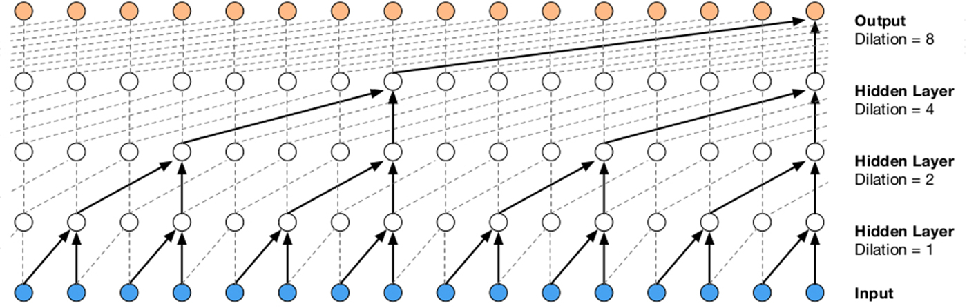
Fig. 18. Causal dilated CNNs used in WaveNet [Reference van den Oord, Deileman, Zen, Simonyan, Vinyals, Graves, Kalchbrenner, Senior and Kavukvouglu116].
The time dilated structure of wavenet also lends itself to an elegant caching-based optimization that allows the network to be evaluated quickly [Reference Paine118].
Nontheless, synthesis systems still rely on many disparate components, which deep neural nets are starting to take over individual parts of. Perhaps the most extreme example of this are the DeepVoice and DeepVoice 2 systems [Reference Arik119,Reference Arik120] in which every single component is implemented as a neural network, some of which are separately pretrained with linguistic data (Fig. 19).
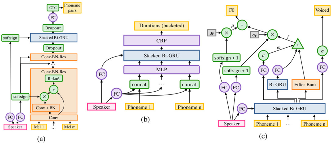
Fig. 19. Neural network equivalents for the acoustic, duration, and pitch models in the DeepVoice systems (from [Reference Arik120]).
Fully end-to-end synthesis using on attention-based encoder-decoder sequence to sequence models were also independently proposed in [Reference Wang121,Reference Sotelo122]. These systems do not rely on external linguistic knowledge, but at the same time it reduces the synthesis problem back into a black box, meaning engineering optimizations and bugfixes become difficult to implement. As of now, we certainly have a long way to go in applying deep learning to speech synthesis.
V. CHALLENGES
As we have seen, the scientific and engineering community have made giant strides in advancing the state of AI. There remains significant challenges that need sustained research and development to address.
A) Understanding DNN
Perhaps one of the biggest source of skepticism for the success of DNN is that there is relatively little theoretical understanding of why they work, and as a result much of the progress has relied heavily on empirical trial-and-error experiments guided by intuition. Researchers have started to study DNN from a more theoretical approach. One of the intriguing studies [Reference Zhang, Bengio, Hardt, Recht and Vinyals123] show that sufficiently DNN are capable of learning randomly labeled, randomly generated images, bring up questions on how DNN generalize, or whether they simply remember and recall everything. The Information Bottleneck [Reference Tishby and Zaslavsky124] theory argues that forgetting is just as important as remembering.
B) Optimizing training for recurrent architectures
The ability to maximally utilize computing resources during training directly impacts the scale of the possible solution space in multiple aspects. For convolutional networks, researchers have successfully designed distributed algorithms that take full advantage of large-scale hardware setups, shortening the training of an IMAGENET neural network from several weeks to an hour. Training recurrent and LSTM neural networks remain a much less efficient process due to the need to expand the network in time, significantly raising the complexity of the training algorithm. Recently, researchers have stated to find ways to remove recurrences altogether to solve problems involving sequences, with promising, novel architectures [Reference Vaswani125].
C) Malicious attacks
Given a known neural network, researchers have shown that it is possible to synthesize images that ‘trick’ the neural network into erroneous responses. More worrisome is that Adversarial examples [Reference Athalye126] can be constructed such that if the image is perturbed slightly the neural network might not be able to classify it correctly even though the image looks the same as before for human observer. This also suggests that there is still significant brittleness in neural networks that are still not fully understood, and it may be possible for malicious parties to exploit this weakness.
D) Challenges in natural language processing
Many classical methods exist where there is no strong analogue in neural network terms. For example in speech recognition, speaker adaptation, and speaker adaptive training [Reference Anastasakos, McDonough, Schwartz and Makhoul95] are classical methods that normalize speaker variability. Currently there are no real analogues in neural networks that can quickly adapt (less than a few seconds) to the characteristics of the individual speaker. This itself is an indication that deep learning still has much to learn and follow from classical ideas.
Other challenging examples are problems in speech and language in which there is no good economical source of large volume data. They are naturally difficult for deep learning, in which having large datasets is crucial to the approach. One example is text normalization – this is necessary precursor stage to synthesis, one example might be to render orthographies of non-standard words such as 6ft, into a word sequence representing how they should actually be read out (e.g. six feet) [Reference Sproat and Jaitly127]. This problem presents a difficulty for deep learning, because firstly, the examples from which to learn such normalizations are very sparse in available large corpora. Second of all, problems such as speech to text or machine translation have natural economic reasons for generating the data – for example, users will pay for closed-captioning of videos, which generate human transcripts of audio as a by-product – which are in turn good labeled data for training speech recognizers. Unlike these problems, there is no economic reason for generating labeled data for text normalization, except to train a text normalization system itself. Other examples for such problems include training speech recognizers and keyword spotters for low-resource languages, in which not more than a few hours of labeled speech can be reasonably obtained, or for example for training speech recognizers for whispered speech, in which there is no economic reason to record large volumes of whispered speech except as part of a need to train a quiet/soft-talking speech recognizer.
VI. IMPACT AND CONCLUSIONS
Beyond yielding good solutions to many longstanding problems, the AI Renaissance is also accompanied, and certainly helped, by a number of positive development in the global scientific and engineering community.
(i) Statistical Testing. One big reason DNN results are convincing is that they are typically trained and tested on large, real-world data sets. It is now virtually a requirement for all newly proposed algorithms and methods to be tested on large data sets, clearly a positive development that introduces an additional degree of rigor to the community.
(ii) Open Source. Another pervasive, positive development is the open sharing of computer source code and data sets, from comprehensive deep learning frameworks like Tensorflow and Caffe to the implementation of algorithms and neural networks that accompany technical reports. This facilitates full reproduction of results reported in publications, and also accelerates understanding of the algorithms since the source codes provide implementation details that are not always appropriate or even possible to fully describe in a technical paper. Open data sets have also made it possible for researchers to reproduce reported results, and also using the data sets as benchmarks for comparing algorithms.
(iii) Open Access. A different but equally important kind of sharing is making technical papers available freely in an Open Access fashion, with arXiv being the most representative repository for scientific papers in the deep learning and computer vision community. While this has made it difficult to enforce anonymity rules in traditional double-blind peer review, the positive is that important results are quickly disseminated, often months ahead of official publication at a conference or journal. Free and open sharing of ideas clearly benefits the scientific and engineering community.
(iv) Automated Algorithms Engineering. The training and validation of neural networks with large data sets can be thought of as highly automated software engineering for algorithms, effectively allowing software to be tested with much more comprehensive test cases than previously possible with manual processes. This also encourages engineers to incorporate more deep learning into their algorithm pipeline, to take advantage of automated testing at scale. The adoption of automated testing even in research laboratories will also accelerate the transfer of new algorithms from the laboratory to production.
As encouraging as the AI Renaissance is, we believe that we have only scratched the surface in what is possible. As researchers and engineers learn to express the treasure trove of insights and ideas accumulated over the past few decades in the new language of AI and deep learning, we will see even harder problems being solved and new solutions put into real-world applications, delivering on the promise of AI.
ACKNOWLEDGEMENTS
The first author would like to thank Irwin Sobel for pointers on the pioneering work at MIT, and Xiaonan Zhou for her work on many of the deep neural network results shown. The second author would like to acknowledge and thank colleagues at Novumind for use of screenshots of several in-house demos as well as assistance in proof-reading the manuscript.
Kar-Han Tan is Head of Product Research & Development at NCS, leading the Singtel Cognitive and Artificial Intelligence Laboratory (SCALE@NTU), a product design and management team, and a full-stack product engineering team. Before, NCS Kar-Han was Vice President of Engineering at NovuMind, where he led the development of artificial intelligence technologies and solutions. At HP, he led the computer vision team that built and launched the Sprout, the first PC with built-in object segmentation, 3D scanning, and real-time collaboration capabilities that leveraged Kar-Han's work on gaze-aware immersive communication at HP Labs. Earlier, he was manager of algorithms group at Epson R&D, where he led the invention of advanced projection and imaging technologies. He has also worked at MERL on Computational Photography. Kar-Han graduated from the National University of Singapore, earned his M.S. from UCLA and Ph.D. from the University of Illinois at Urbana-Champaign, where he was a Beckman Institute Graduate Fellow.
Boon Pang Lim (M’11) is the Lead for Speech Technology at Novumind Inc; formerly a Research Scientist at the Institute for Infocomm Research (I2R). Dr Lim's research interests are in automatic speech recognition and applications, with focus on acoustic modeling in various conditions such as low-resource languages, whispered speech, and Singapore Chinese dialects. He was involved in building several prototypes for industry while at I2R, including cloud-based ASR for Malay, Tamil, Mandarin and English, and keyword search. Dr. Lim is the recipient of several awards and government scholarships, including the NUS High School and Singapore MOE Outstanding Mentor Awards (2013-2016); as well as the Public Service Commission Overseas Merit Scholarships (PSC-OMS) and National Science Scholarship (NSS) from the Singapore Government. He received the B.Sc, M.Sc, and Ph.D. degrees in Electrical and Computer Engineering (ECE) from the University of Illinois at Urbana-Champaign (UIUC) in 2000, 2001, and 2011, respectively.


 Open access