


Introduction
Changes in global climate and sea level are intricately linked to changes in the area and volume of polar ice sheets. Thus, melting of the ice sheets may severely impact the densely populated coastal regions on Earth. Melting of the West Antarctic ice sheet alone could raise sea level by 5 m. As this ice sheet rests largely on bedrock below sea level, it is potentially unstable and could, hypothetically, disintegrate within the next 100 a (Reference MercerMercer, 1978; Reference Thomas, Sanderson and Rose.Thomas and others, 1979). In spite of their importance, the mass balances (the net gains or losses) of the Antarctic ice sheets are still poorly known.
Intensive studies have been made of ice streams draining the West Antarctic ice sheet into the Ross and Ronne Ice Shelves, but relatively little is known about the ice streams and glaciers draining the ice sheet along the Marie Byrd Land coast. The most conspicuous ice streams in that area are Pine Island and Thwaites Glaciers. They have been studied by Hughes (1981), Reference Crabtree and Doake.Crabtree and Doake (1982), Reference Williams, Ferrigno, Kent and SchoonmakerWilliams and others (1982), Reference Lindstrom and Tyler.Lindstrom and Tyler (1984), and Reference Ferrigno, Lucchitta, Mullins, Allison, Allen and Gould.Ferrigno and others (1993). Hughes (1981) suggested that the loss of an ice shelf in Pine Island Bay, pinned by islands, may have caused Pine Island and Thwaites Glaciers to surge, resulting in down-draw of their drainage basins and retreat of the grounding lines. Indeed, Hughes (1981) called Thwaites and Pine Island Glaciers the “weak underbelly of the West Antarctic ice sheet”. More recent studies have focused on mass balances of these glaciers (Reference Crabtree and Doake.Crabtree and Doake, 1982, Reference Lindstrom and Hughes.Lindstrom and Hughes, 1984), which were found to be highly positive. Our study reports on new velocity measurements for Pine Island Glacier (Fig. 1) and may help to clarify the mass-balance issue for future studies.

Method
We successfully used sequential Landsat images (acquired as much as 20 years apart) to obtain average velocities by tracking crevasse patterns on the floating tongue of outlet glaciers and ice streams (Reference Lucchitta and Ferguson.Lucchitta and Ferguson, 1986; Reference Lucchitta, Mullins, Allison. and Ferrigno.Lucchitta and others, 1993, Reference Lucchitta, Mullins, Smith. and Ferrigno.1994b). However, Landsat images have disadvantages: the early images have low (about 80 m per pixel) resolution; the long polar winter night reduces acquisition opportunities; and cloud cover impedes recognition of features. For this study we used ERS-1 SAR images (European Remote-Sensing Satellite, Synthetic Aperture Radar), which have 30 m resolution (12.5 m per pixel), image quality independent of season and cloud cover and similar viewing conditions if nearly identical orbital paths and image-frame locations are used in sequential images. For example, the high resolution of ERS-1 images permits the identification of small crevasses and other patterns on ice streams or ice sheets above or at the grounding line (where the ice leaves land and begins to float), whereas the lower resolution of the early Landsat Multispectral Scanner (MSS) images permits identification of only the large patterns in the floating part of the ice (tongues or shelves). Knowledge of velocities at the grounding line allows calculation of discharge rates from the ice sheets, provided the cross-sectional area of the ice streams is known.
We acquired two sets of consecutive, geocoded ERS-l SAR images—one set from 9 February, the other from 4 December 1992 (Table 1; Fig. 1). Geocoded images are in Universal Polar Stereographic projection using the WGS 1984 ellipsoid and are processed to correct for a reference mean elevation level assigned to the frame. The displacement in range within a frame is 2.3 times the elevation difference between the actual elevation of the point and the reference elevation level of the frame (Reference Roth, Hügel, Kosmann, Matschke. and Schreier.Roth and others, 1993). The range displacement is similar in our repeat images, as they have close orbital-path and frame locations and are processed to the same reference elevation levels by the German Processing Facility (D-Paf). Also, the glacier surface slopes gently (about 350 m per 100 km according to the reference elevations used (Table 1); therefore, tracked points that moved down-glacier for 1 km horizontally dropped about 3.5 m vertically. This slope creates a range error of less than 1% (about 8 m over the 1 km distance).
Table 1. Image specifications (ERS-1 SAR, C-band, geocoded)

We co-registered the images acquired at an interval of 10 months by (1) matching fixed points, such as nunataks (land masses projecting through the ice), and (2) using the furnished coordinates based on orbital parameters. When using the first method, the images matched so well that the broad outlines of nunataks sufficed for co-registration and no special algorithms needed to be applied for geometric corrections. Therefore, we have no statistics on residual errors of co-registration points. When using the second method for co-registration, we obtained the same fit. The observation that co-registration by ground features and by orbital parameters yielded the same fit increased our confidence in the nominal locations of the images on the ground, which is accurate to 50 m according to Roth and others (1993). A hypothetical 50 m error in nominal location between the two images would result in a 5% error in measured displacement between a tracked point that moved a distance of 1 km; the larger the displacement, the less the percentage error. Our displacements for the central parts of Pine Island Glacier range from about 0.9 to 1.8 km for the 10 month interval between image acquisitions, so a hypothetical mismatch of 50 m in image location would result in an error of less than about 5%. To reduce speckle, we compressed the images to 25 m per pixel by averaging squares of four pixels.
Initially, visually tracked crevasse patterns (Reference Lucchitta, Mullins, Allison. and Ferrigno.Lucchitta and others, 1993) yielded a preliminary set of velocity values (Reference Lucchitta, Smith, Bowell. and Mullions.Lucchitta and others, 1994a). Later, an automated cross-correlation program developed by Reference Bindschadler and Scambos.Bindschadler and Scambos (1991) and Reference Scambos, Dutkiewicz, Wilson. and Bindschadler.Scambos and others (1992), which gives the displacements of crevasses or other recognizable patterns that move with the ice, allowed us to calculate the velocities from the distances moved in the given time interval. Displacement vectors were then projected onto an image of the glacier (Fig. 2). To obtain the distribution of average velocities over the length of the glacier, we also measured the distance from the location of each moving point on the earlier image of the pair to the position of the grounding line as inferred in figure 1 of Reference Crabtree and Doake.Crabtree and Doake (1982). To closely duplicate their location, we carefully inspected an enhanced version of the Landsat image used in their figure and transposed the line onto the radar image. The measurement results are represented in a graph (Fig. 3) that displays the average velocities per given time interval vs the distance to the grounding line for all measured points on the glacier.

Fig. 2. Upper part of Pine Island Glacier. Movement toward bottom; north toward left. ERS-l 2970-5589, 9 February 1992. Small white lines are displacement vectors showing movement of glacier in 10 month interval. Dashed line is grounding line as inferred by Reference Crabtree and Doake.Crabtree and Doake (1982).
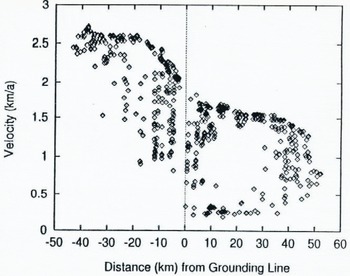
Fig. 3. Glacier velocity plotted against distance from grounding line of Reference Crabtree and Doake.Crabtree and Doake (1982). Positive values in grounded part of glacier, negative values in floating part. Scatter reflects velocity differences across width of glacier. Note rapid increase in velocity starting near grounding line and extending 20 km down-glacier.
Discussion
Observations
The images show remarkable curvilinear crevasse patterns across the entire glacier, where the flowlines converge toward a more confined channel (Fig. 4). The crevasses form a concave (downstream) fracture pattern that is distorted to a convex pattern by the faster flow in the center of the ice stream. This set of Crevasses has never been described. Perhaps it is covered by a thin layer of snow and is visible only on radar images. A new set of crevasses can be seen at the upstream end of the December 1992 image, shown in green on this multi-temporal image. The set apparently formed in the interval between the two image acquisitions.

Fig. 4. Excerpt of multi-temporal composite image of Pine Island Glacier, showing curvilinear fracture pattern. Movement toward bottom left; north toward top left. ERS-1 2970-5589, 9 February 1992, in red; ERS-1 7251-5589, 4 December 1992, in green. Radar illumination from bottom; ascending orbit. Matched features in images show in yellow, unmatched features such as crevasses in red or green. Note conspicuous new crevasse set in green at top (arrow) and distortion of crevasses down-glacier from concave to convex by faster ice movement in center.
The terminus of the glacier retreated about 4 km in the 10 months between image acquisitions, as seen in the multi-temporal image of Figure 5. The figure also shows that the glacier apparently calved an iceberg about 5 km wide between the February and December image acquisitions; this loss has already been partly offset by an advance of the calving front by about 2 km since the acquisition of the February image. Overall, the position of the glacier from between 1973 (Landsat image) and 1992 (ERS-l images) has not changed substantially; the apparent setback and rate of retreat or advance depends on the location of the glacier front at the time of image acquisition. For instance, a retreat of 0.2–0.3 km a−1 is suggested when measuring from the contact of the glacier front with open water in 1973 to the position of the post-calving front shown in February 1992 (Fig. 5). However, placing the 1973 ice front at a fracture marking a future calving front and measuring from there to the February 1992 post-calving position, shows the setback in the 19 years to be only about 1 km, a rate of retreat of about 50 m a−1. When the 1973 position of the fracture is compared with the readvanced glacier front in the December 1992 image, the glacier has actually moved beyond this fracture by a few tens of meters. Our observations show that only the tracking of immediate post-calving positions on this last-moving glacier will reliably establish retreat rates and trends.

Fig. 5. Multi-temporal composite image of Pine Island Glacier front. Movement toward bottom; north toward left. ERS-I 2970-5607, 9 February 1992, in red; ERS-1 7251-5607, 4 December 1992, in green. Radar illumination from bottom right; ascending orbit. Note glacier front of February 1992 (red); partly attached tabular iceberg extending from red front to thicker, conspicuous green line near front; and absence of iceberg and readvance of glacier from thicker green line to front of December 1992 (yellow).
Our observations support a smaller recent retreat rate, if any, than the 0.8 km a−1 reported by Reference Kellogg and Kellogg.kellogg and Kellogg (1987) from positions of the glacier front in 1966 (photographic observation), 1973 (Landsat observation) and 1985 (inspection on location). Reference Kellogg and Kellogg.kellogg and Kellogg (1987) contend that this rate of retreat supports the existence of an ice shelf in Pine Island Bay less than 100 years ago. Close monitoring of future calving events is needed to verify their hypothesis.
Velocities
We measured average velocities for the 10 month period on both the grounded and floating parts of Pine Island Glacier (Fig. 2). The velocities for the fast-moving central parts of the glacier range from about 1.3 km a−1 about 50 km above the grounding line to an interpolated 1.9 km a−1 at the grounding line to 2.6 km a−1 beginning about 20 km below the grounding line on the floating part of the glacier {Fig. 3). The scatter of points on the graph (Fig. 3) corresponding to 50 km above the grounding line is due to the low velocities near the margin of the glacier recorded by the automated cross-correlation program (Fig. 2). Even though trackable crevasses appear to be present at the grounding line, they were not recognized by the program.
The grounding line, commonly considered to mark the place where the glacier separates from the ground and begins to float, was inferred by Reference Crabtree and Doake.Crabtree and Doake (1982) to lie within a region of rolling topography on the glacier surface. They based this placement on profiles of two radio-echo-sounding flights along the glacier. The location is surprising, as visual inspection of the images suggests that the grounding line lies 20 km farther down-glacier, where the rolling topography gives way to an apparently level surface with many large transverse crevasses. This 20 km segment coincides with a rapid increase in velocities. In the grounded part above the inferred grounding line of Reference Crabtree and Doake.Crabtree and Doake (1982), velocities increase only gradually, supporting their suggestion that the line is held on a rock bar. In the floating part below the 20 km segment, velocities also increase very little. The data suggest that this transitional segment marks a grounding zone, where the glacier is only partially or lightly grounded. This transitional segment also coincides with a zone where, according to Reference Crabtree and Doake.Crabtree and Doake (1982), Fig. 2a), surface elevations on the glacier have levelled out but lie about 50 m above the downstream, floating ice and are separated from it by a scarp. Perhaps the region is analogous to what has been termed, informally, an “ice plain” at Ice Stream B (personal communication from R. Bindschadler. 1994).
The velocities we determined for the floating part of the glacier are somewhat higher than velocities previously established. Reference Crabtree and Doake.Crabtree and Doake (1982) used Landsat images of 1973 and 1975 to measure an average velocity at the ice front of 2.1±0.2 km a−1. Reference Williams, Ferrigno, Kent and SchoonmakerWilliams and others (1982) measured 2.2, and Reference Lindstrom and Tyler.Lindstrom and Tyler (1984) approximately 2.4 km a−1, also at the front. The latter authors found velocities of about 2.2 km a−1 in four measurements approximately 30 km upstream from the terminus, velocities of about 2.1 km a−1 in one measurement approximately 40 km upstream, and velocities of about 2.0 km a−1 in one measurement approximately 50 km upstream. Only this last point overlaps with our measurements. Reference Lindstrom and Hughes.Lindstrom and Hughes (1984) used a Velocity of 0.712 km a−1 at the grounding line, referring to measurements made in Reference Lindstrom and Tyler.Lindstrom and Tyler (1984). We do not know if the discrepancy between our measurements and earlier ones is caused by an actual increase in glacier velocity within the last 10–20 years or if our values reflect different and perhaps more accurate measurements because of a new image set that has better internal geometry, location accuracy and co-registration.
Mass balance
Mass balances for Pine Island Glacier have been calculated by Reference Crabtree and Doake.Crabtree and Doake (1982) and Reference Lindstrom and Hughes.Lindstrom and Hughes (1984). Reference Crabtree and Doake.Crabtree and Doake (1982) defined the drainage basin of Pine Island Glacier by surface elevations based on pressure altimetry and obtained the accumulation rate from the literature (Reference GiovinettoGiovinetto, 1964; Reference Bull and QuamBull, 1971). They calculated the discharge based on the velocity, width and thickness of the floating ice front after appropriate model-based adjustments, and they arrived at a mass balance of +61±30 × 1012 kg a−1. Reference Lindstrom and Hughes.Lindstrom and Hughes (1984) defined the drainage basin by surface elevations given in Reference DrewryDrewry (1983), and their accumulation rates were obtained from snow-pit stratigraphy along tractor traverses (input mass flux 65.9 × 10¹² kg a−1). They calculated the discharge at the grounding line by using a velocity (0.712 km a−1) and width (26.2 km) from their own Landsat-image measurements and a mean ice thickness (1.564km) from Crabtree and Doake’s (1982) radio-echo-sounding data (ice density 900 kg m−3). They obtained a mass balance of +40×12 kg a−1 and assigned an uncertainty of 7 Gt a−1 to this value (no reasons given). They further explained that the width of 26.2 km includes only the ice-stream segment between the marginal shear zones, and thus, they asserted, only the inferred plug flow in the central part of the glacier was considered for the discharge calculation.
Because Lindstrom and Hughes’s (1984) discharge calculation was performed for the same grounding line as that used in this study, our revised velocity value of 1.9 km a−1 for the grounding line can be applied to their other output parameters. Thus, we computed a discharge of +70 × 1012 kg a−1. Combining this discharge flux with Lindstrom and Hughes’s input flux, we arrived at a mass balance of −4.2 Gt a−1. These results are at odds with earlier results in that they suggest that Pine Island Glacier is nearly in balance. However, the radio-echo-sounding cross-profile in Fig. 3b of Reference Crabtree and Doake.Crabtree and Doake (1982), giving ice thickness, is located 20 km downstream from the grounding line used in this report (Fig. 2) and used by Reference Lindstrom and Hughes.Lindstrom and Hughes (1984), so the cross-sectional area of the glacier at the grounding line is not known precisely. Thus, the ice cross-sectional area used in the discharge calculations for the grounding line is questionable. If the glacier-bottom cross-sectional shape were similar to the one profiled 20 km downstream in Reference Crabtree and Doake.Crabtree and Doake (1982), showing sloping sides, then the cross-sectional area would be less than that used by Reference Lindstrom and Hughes.Lindstrom and Hughes (1984). Also, our measurements indicate that Pine Island Glacier may not exhibit plug flow, so slower velocities near the ice-stream margins must be taken into account. All these considerations would decrease the mass flux across the grounding line, thus shifting the balance in a positive direction.
In summary, our study shows that the velocities of Pine Island Glacier may be somewhat faster than previously thought and that, consequently, the mass balance may be less positive than indicated by earlier studies. However, the shape and flow regime of the glacier at the grounding line are not yet established in sufficient detail to allow for precise discharge calculations, and uncertainties in the input parameters remain large, so that, overall, the mass balance of Pine Island Glacier remains poorly known.
Acknowledgements
We are grateful to R. Bindschadler and T. Scambos, who made the automated cross-correlation program available to us. We also thank J. Bowell and E. Cisneros, who aided in the computer processing. Reviews by R. Bindschadler, H. Kieffer, J. Kargel and an anonymous reviewer helped improve the manuscript. The ERS-l images were made available at no cost by the European Space Agency. The research was funded by the U.S. Geological Survey with contributions by NASA’s Earth Observing System.


