Introduction

Airborne and Satellite Radar Datasets Are Important Tools For Mapping Conditions Within Glaciers and Ice Sheets. Most Satellite Studies Have Focused On Surface Elevation, Motion and Facies Of Ice Sheets (Reference Bindschadler and VornbergerBindschadler and Vornberger, 1992; Reference Fahnestock, Bindschadler, Kwok and JezekFahnestock and others, 1993; Reference Jezek, Gogineni and ShanablehJezek and others, 1994; Reference Joughin, Winebrenner, Fahnestock, Kwok and KrabillJoughin and others, 1996; Reference Rignot, Forster and IsacksRignot and others, 1996). Over Mountain Glaciers, Radar Has Also Been Used To Measure Motion, Surface Elevation, Snow Facies and Glacier Extent (Reference Rignot, Forster and IsacksRignot and others, 1996; Reference Hall, Williams, Barton, Smith and GarvinHall and others, 2000; Reference Fatland and LingleFatland and Lingle, 2002; Reference König, Wadham, Winther, Kohler and NuttallKönig and others, 2002; Reference Wolken, Sharp and WangWolken and others, 2009; Reference Atwood, Meyer and ArendtAtwood and others, 2010). The Penetration Depths Of L- and C-Band Radar Signals (1–2 and 4–8 Ghz, Respectively) Have Been Used To Study The Temporal Coherence Necessary For Ice Velocity Mapping (Reference Rignot, Echelmeyer and KrabillRignot and others, 2001) and To Investigate The Causes Of Radar Backscattering (Reference LangleyLangley and others, 2008), But No Satellite Study Of Mountain Glaciers Has Investigated The Information Revealed By Spatial Patterns In Penetration Depth As They Relate To Near-Surface Thermal Properties Of The Ice.

The apparent penetration depth (i.e. the difference between the glacier surface elevation and the depth of scattering horizons) of low-frequency (0.1–0.3 GHz) radar waves is typically used to infer the near-surface thermal regime of glaciers (Reference BjörnssonBjörnsson and others, 1996; Reference MooreMoore and others, 1999; Reference MurrayMurray and others, 2000; Reference Pettersson, Jansson and HolmlundPettersson and others, 2003; Reference NavarroNavarro and others, 2009; Reference Gusmeroli, Murray, Jansson, Pettersson, Aschwanden and BoothGusmeroli and others, 2010, Reference Gusmeroli, Jansson, Pettersson and Murray2012). Liquid water existing at the boundary between cold and temperate ice produces spatially continuous radar scattering horizons sensed by low-frequency radar. By mapping the distribution of the radar scattering horizons across the surface of a glacier, it is possible to infer distinct near-surface thermal regimes and track their evolution through time.

In July 2010, Fugro EarthData Inc. collected dual-band (7–12GHz X-band and 0.4 GHz P-band) interferometric synthetic aperture radar (InSAR) data over portions of Alaska, USA, as part of a regional mapping initiative. Although the X-band data were used for most of the surface mapping, P-band observations were also acquired, primarily to map the terrain height beneath the vegetation canopy. Here we analyze the spatial distribution of the difference between X- and P-band elevations (the apparent P-band penetration depth, _P ) over Kahiltna Glacier, a large mountain glacier located in the Alaska Range. We compare our airborne measurements with a 100MHz ground-based radar survey located in the upper ablation area of the glacier. Our airborne observations span a wide range of climate regimes, from near-polar conditions with negligible melt above ∼4000m elevation, to a temperate climate with several meters of ice melt per year at ∼300m elevation. We interpret variations in _P across these climatic zones in terms of the near-surface thermal regime of the glacier. Our observations provide a framework for airborne mapping of glacier thermal structure and for tracking the response of glaciers due to environmental changes.

Methods

We use two different types of radar systems: dual-band airborne InSAR, used to investigate glacier-wide variations in P-band radar penetration depth, and ground-penetrating radar (GPR), used for detailed field observations at one location on the glacier. The main difference between InSAR and GPR is that the former retrieves interferometrically measured topographic heights (e.g. Reference Rignot, Forster and IsacksRignot and others, 1996, Reference Rignot, Echelmeyer and Krabill2001), whereas the latter retrieves radar returns caused by englacial features (e.g. Reference Gusmeroli, Murray, Jansson, Pettersson, Aschwanden and BoothGusmeroli and others, 2010, Reference Gusmeroli, Jansson, Pettersson and Murray2012; Reference CampbellCampbell and others, 2012).

GeoSAR

The GeoSAR system was developed from 1998 to 2003 as a joint effort of the NASA Jet Propulsion Laboratory (JPL) and Fugro EarthData under sponsorship of the US Defense Advanced Research Projects Agency-National Geospatial-Intelligence Agency (DARPA-NGA). It is a unique dual-band, dual-sided, single-pass airborne interferometric mapping radar designed to efficiently map both the top of vegetation canopies and the terrain beneath the canopy. The former is achieved by the X-band radar, with a wavelength of ∼3 cm, and the latter by the P-band radar, with a wavelength of ∼86cm. System parameters are provided in Table 1.

Table 1. GeoSAR acquisition parameters. GeoSAR was flown on a Gulfstream II jet from 10 to 31 July 2010 at an altitude of 11 900 m with a speed of 450 knots (∼830kmh^–1)

In July 2010, the GeoSAR was flown as part of the Alaska statewide digital mapping initiative (SDMI) in an area between Fairbanks, Anchorage and Mount McKinley. The main objective of the project was to create two 5 m, mid-accuracy (elevation root-mean-square error <1.85 m) digital elevation models, one a digital surface model (DSM_X) showing the top of the canopy, and one a digital terrain model (DTMP) showing the terrain beneath the canopy. The GeoSAR X-band swaths (typically four) were combined into a single mosaic for the DSM_X. The P-band data were combined into a single mosaic to obtain an estimate of ground elevation beneath vegetation (DTM_P). In the mountainous terrain above the treeline, X-band data were used to create the DTM_P, where it was noticed that the P-band radar penetrated the surface of glaciers by tens of meters. In this paper, we report the spatial variation of the observed 5_P = DSM_X- DTM_P; i.e. the apparent GeoSAR P-band penetration depth into firn and glacier ice of Kahiltna Glacier (Figs 1 and 2).

Fig. 1. Location of our study and map of Kahiltna Glacier, Alaska Range. Black shading indicates the debris-covered portion of the glacier.

Fig. 2. Details of P-band InSAR penetration depths, _P, on Kahiltna Glacier. (a) _P over the entire glacier. (b) Close-up detail of the boundary between percolation zone (blue colors: high _P ) and wet snow zone (red colors: low _P ). (c) Boundary between the wet accumulation area and the upper ablation area with cold surface ice. (d) Portion of the lower ablation area, with visible debris bands with very low _P. (e-g) show _P values along the transects indicated in (b-d). The approximate location of the 20 year averaged equilibrium-line altitude (ELA, ∼1900ma.s.l.; Reference Burrows and AdemaBurrows and Adema, 2011) is indicated.

Ground-penetrating radar

Detailed 100 MHz GPR data were collected in the middle of the ablation area, at an elevation of 1200 m (see Fig. 1 for location) in April 2011, using a commercially available pulseEkko Pro system. The transmitter and receiver were installed 1 m apart on a wooden sledge which was towed on the snow surface along four 100 m long straight transects (Fig. 3a). Two hundred radar traces per transect were acquired by holding the radar system motionless every 0.5 m. The GPR survey was positioned with a handheld Garmin GPS system. The accuracy of the positioning was on the order of ±10m. Snow depths were measured using a graduated avalanche probe every 5 m along each GPR profile. The snow survey yielded an average snow depth of 1:85 ± 0:25 m, and this value was used to correct the radar travel times (Reference Pettersson, Jansson and HolmlundPettersson and others, 2003; Reference Gusmeroli, Jansson, Pettersson and MurrayGusmeroli and others, 2012). We identified the transition between transparent cold ice and scatterer-rich temperate ice on each radargram (Fig. 3b1-b4). The one-way travel time, t, for a radar return from the base of the cold layer can be used to calculate the thickness of the cold surface layer (CSL), d_csl:

(1)

Fig. 3. The cold surface layer on Kahiltna Glacier, as detected by a detailed GPR survey. (a) Sketch of the 100 MHz GPR lines; arrows indicate survey direction. (b1-b4) 100 MHz GPR lines acquired in the upper ablation area, showing the radar stratigraphy with a distinct topmost layer of transparent cold ice overlying a lower layer of ice rich in scatterers. (c) Box plots of the thickness of the cold surface layer derived from each GPR profile, with the red box plot, labelled , as the mean penetration depth of the P-band InSAR in the GPR study area (inside the square). Error bars in this plot relate to the spatial variability in cold surface layer thickness. Cold surface layer thickness and the depth scale in the GPR profiles were derived using radar speeds of 0.24 and 0.168 m ns^–1 for snow and ice, respectively (Reference RobinRobin, 1975; Reference Gusmeroli, Murray, Jansson, Pettersson, Aschwanden and BoothGusmeroli and others, 2010, Reference Gusmeroli, Jansson, Pettersson and Murray2012).

By using values of radar speed in snow, v _snow = 0.24± 0.02 m ns^–1 (Reference RobinRobin, 1975), and radar speed in the CSL, v _csl = 0:168 ± 0:002 m ns^–1 (Reference Gusmeroli, Murray, Jansson, Pettersson, Aschwanden and BoothGusmeroli and others, 2010) we can calculate the CSL thickness, d _csl, and the associated uncertainty. Uncertainties in the radar speeds in snow and ice, v _snow and v _csl, include a broad spectrum of snow densities (0.3 ± 0.1 gcm^-3) and observed experimental errors, respectively. These uncertainties typically result in a worst-case scenario error of ±3 m in measured CSL thickness (Reference Gusmeroli, Jansson, Pettersson and MurrayGusmeroli and others, 2012).

Results

The GeoSAR imagery (Fig. 2) shows variable InSAR characteristics over the glacier. We report on results from selected areas along the glacier center line, where the ice is generally free of crevasses and debris. Results can be divided into five different zones: (1) the upper part of the accumulation area (>2500m), where _δP is high (18±3m); (2) the lower accumulation area (1700-2500 m), where _P drops to 1 0 ± 4 m ; (3) the upper part of the ablation area (1000-1700 m), where _P is highest (34 ± 4 m); (4) the lower part of the ablation area (500-1000 m on bare ice) with _P = 23 ± 3 m; and (5) the debris-covered part of the ablation area (near the terminus, at elevations <500m), where _P is lowest (5-10 m). The most notable features of these results are spatial variability of _P and the very high values in the upper ablation area.

There are two prominent transitions between zones: one is located in the uppermost area of the glacier (Fig. 2b), and the second is located just below the estimated equilibrium-line altitude (ELA; Fig. 2c). Sample cross sections of the _P map are provided in Figure 2e (a region of relatively low penetration in the accumulation area), 2f (a region of very high penetration in the ablation area) and 2g (a region with low penetration at the margin of the tongue in the ablation area). In the lower ablation area, there are marginal zones and longitudinal stripes of low penetration, likely caused by the presence of supraglacial debris (Fig. 2d).

Our ground observations show that the thickness of the CSL at Kahiltna Glacier is 12-23 m (Fig. 3a and b1-b4). In the GPR study area there is pronounced spatial variability (average CSL thickness is as low as 12 m across CD and as high as 23 m across AB). The CSL thickness at this location is of similar magnitude to the _P averaged over the GPR study area (Fig. 3c). Surface scatterers, only observable in the across-glacier profiles (BC and DA), are likely caused by along-glacier-oriented features (i.e. supraglacial channels and fractures).

Discussion

Our GPR data (Fig. 3) show the presence of a clear radar stratigraphy in the ablation area of Kahiltna Glacier, which we propose to be a 12-23 m thick layer of cold ice overlying the temperate core of the glacier. Locally, cold ice can reach a thickness of 20-23 m (our migrated GPR data also show similar, consistent thicknesses). Spatial variability in CSL thickness is likely affected by the presence of englacial debris and other features (water and air bodies). Here we hypothesize that InSAR _P is also controlled by the thermal properties of the glacier ice. Cold glacier ice is transparent to radar waves, but the signal is scattered at the temperate side of the cold-temperate transition surface (CTS), a relatively sharp boundary at which the crystalline water content rises from zero to ∼0.5% (Reference Pettersson, Jansson and BlatterPettersson and others, 2004; Reference Gusmeroli, Murray, Jansson, Pettersson, Aschwanden and BoothGusmeroli and others, 2010). Scattering due to water bodies impedes radar penetration (Reference Pettersson, Jansson and HolmlundPettersson and others, 2003; Reference Gusmeroli, Jansson, Pettersson and MurrayGusmeroli and others, 2012), such that _P is likely affected by the position of the CTS. Reference Rignot, Echelmeyer and KrabillRignot and others (2001) reported InSAR L-band penetration depth, _L, on exposed bare ice up to 60-120 m in the colder sector of the Greenland ice sheet. In contrast, on a temperate glacier in Alaska, _L was 1 2 ± 6 m (Reference Rignot, Echelmeyer and KrabillRignot and others, 2001). The penetration depth of radar signals appears to be highly sensitive to the thermal state of the ice mass (low penetration in temperate ice; high penetration in cold ice).

Our GPR study area was located in the lowermost zone of the high-_δP zone in the middle of the ablation area. A surface layer of cold ice in this area is to be expected (Reference PatersonPaterson, 1972). Reference Harrison, Mayo, Trabant, Weller and BowlingHarrison and others (1975) reported, using direct temperature measurements, a CSL of this kind at similar altitudes on Black Rapids Glacier in the Alaska Range. The CSL of Black Rapids Glacier was also recognizable by its distinct transparency in the radargrams of Reference Arcone and YankielunArcone and Yankielun (2000).

Observed spatial patterns in _P appear to match the spatial distribution of glacier facies zones that typically occur on a mountain glacier. In the highest portion of many glacierized mountains, the summer temperatures may rarely exceed 0°C. In these conditions, the surface remains dry and consists entirely of dry, cold firn and cold glacier ice (z1 in Fig. 4b; Reference BensonBenson, 1961; Reference PatersonPaterson, 1972). At lower elevations, but still in the accumulation area, some of the annual snow cover is melted, such that meltwater percolates through the porous snow/firn aquifer and the cold content of the snow/firn pack is quickly removed by the release of latent heat as the meltwater refreezes. The snowpack at the end of the summer becomes temperate, so that this zone is composed of temperate firn and ice (z2 in Fig. 4c). Between z1 and z2 there is a transitional zone called the percolation zone. Reference CampbellCampbell and others (2012) conducted snow-coring and extensive 100MHz GPR surveys in z1 of Kahiltna Glacier, and suggested that the uppermost boundary of the wet snow area is located at ∼2600m elevation. The conclusions of Reference CampbellCampbell and others (2012) were derived by noticing sporadic melting and a lack of scattering in their GPR images. Our interpretation of the boundary between z1 and z2 (the boundary between the percolation and the wet snow zone in Fig. 4) agrees with this elevation. Above the ELA (Fig. 4d) there is firn, whereas below the ELA there is bare glacier ice. On bare ice the latent heat release from refreezing does not occur; the cold content of the ice is therefore difficult to remove and a permanently cold surface layer can exist (z3 in Fig. 4e). At lower elevations, in the lower ablation area, the cold content of the uppermost ice is removed by high ablation. In this area (z4 in Fig. 4f), the summer surface of a glacier is therefore temperate (Reference PatersonPaterson, 1972).

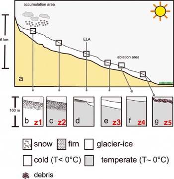
Fig. 4. Near-surface glacier thermal regimes discussed in this paper. (a) Idealized sketch of a glacier of the Alaska Range that originates at high elevation (∼3000m) and terminates near the boreal forest (∼300m). (b) Dry snow zone. (c) Wet snow zone. (d) Vicinity of the ELA. (e) Ablation area with a CSL (f) The ablation area with temperate surface ice in the summer. (g) Debris-covered parts of the ablation area.

The GPR-derived CSL thickness compares well with the InSAR S _P (Fig. 3), even though the two surveys were collected in two different epochs (summer 2010 InSAR, spring 2011 GPR). This singular GPR survey location provides the only data currently available, precluding further speculation about the spatial variability of the CSL on Kahiltna Glacier. However, as observed in Scandinavia (Reference Pettersson, Jansson and HolmlundPettersson and others, 2003; Reference Gusmeroli, Jansson, Pettersson and MurrayGusmeroli and others, 2012), summer ablation reduces CSL thickness, providing a potential explanation for the ∼30% lower S _P on bare ice in the lower ablation area than in the upper zone (Fig. 2f and g).

We hypothesize that our _P map represents a useful snapshot of the thermal regime of Kahiltna Glacier in summer 2010. The spatial extent of these zones, together with the penetration depths of the radar signal, will likely change in the future in response to climatic changes. From our interpretation, we are able to constrain some of the area that is internally accumulating (z2) which can provide valuable information for mass-balance studies that require corrections for internal accumulation (Reference Schneider and JanssonSchneider and Jansson, 2004). It is important to mention that our apparent _P is likely an underestimate of the real P-band penetration depth, because X-band penetration depth in dry polar firn is in the 5–10m range (Reference Davis and PoznyakDavis and Poznyak, 1993; Reference Rott, Sturm and MillerRott and others, 1993). Nonetheless, given the fact that X-band penetration depth should be significantly lower on a glacier in Alaskathan on cold and dry polar firn, we expect differences <5 m.

Conclusions

InSAR is a promising tool for deducing the near-surface thermal state of glaciers, especially those in which a relatively thin CSL exists. We observed high penetration depths of InSAR P-band radar at the upper ablation area of a large mountain glacier, a zone in which we would expect a CSL to exist. This layer likely comprises ice cooled during winter months and not sufficiently heated by the latent heat of refreezing (occurring at elevations above the ELA) or removed by sufficiently high levels of surface melting. Although our observations agree with borehole temperature measurements at similar elevations of a nearby glacier, future efforts should confirm our interpretations through direct borehole temperature observations on Kahiltna Glacier. Direct comparisons between concurrent ground and airborne observations, each sampling similar radar frequencies, will also lend greater confidence to our observations.

We expect that future InSAR observations on Kahiltna Glacier will change according to the climatic changes experienced by the glacier. For example, in the case of a warming climate, we hypothesize that the percolation zone will become warmer ( _P will decrease), the boundary between z2 and z3 will migrate to higher elevation ( _P will decrease below the ELA) and the CSL of z3 will be eroded by ablation ( _P will decrease in z3). We suggest that future repeated (annual or multi-annual) GeoSAR acquisitions over glaciers could be used to detect changes in thermal structure that can be related to changes in climate. Given that the P-band signal penetration is high (>10m), the signal probes the englacial regime that is unaffected by seasonal/annual air temperature variations (Reference PatersonPaterson, 1972). In this respect there may be no differences in undertaking GeoSAR surveys in summer or winter.