


1. Introduction
Sea ice plays an important role in heat exchange between the ocean and atmosphere due to its impact and feedback on the transfer of heat, moisture and momentum across the ocean–atmosphere interface (Rinke and others, Reference Rinke, Maslowski, Dethloff and Clement2006; Dieckmann and Hellmer, Reference Dieckmann and Hellmer2010). Polar regions also show high sensitivity to climate change due to the high reflectivity of ice compared to ocean water. This ice-albedo feedback mechanism is a factor that contributes to high polar sensitivity to warming (Holland and others, Reference Holland, Bitz and Weaver2001; Screen and Simmonds, Reference Screen and Simmonds2010). The sea ice of the two polar regions has experienced different patterns of change since the late 1970s (Turner and Overland, Reference Turner and Overland2009; Simmonds, Reference Simmonds2015). In the Arctic, there has been a remarkable reduction of sea-ice extent and thickness (Kwok and Rothrock, Reference Kwok and Rothrock2009; Simmonds, Reference Simmonds2015; Meier, Reference Meier2017). By contrast, based on passive microwave satellite data, a slight increase in Antarctic sea-ice extent has been observed since the late 1970s (Zhang, Reference Zhang2007; Parkinson and Cavalieri, Reference Parkinson and Cavalieri2012) until a sharp decline occurred in late 2016 (Stuecker and others, Reference Stuecker, Bitz and Armour2017; Turner and others, Reference Turner2017; Kusahara and others, Reference Kusahara, Reid, Williams, Massom and Hasumi2018) leading the satellite era minimums observed in 2017 and 2018 (Parkinson, Reference Parkinson2019). Much of the previous extent increase had occurred in the region of the Ross Sea (Parkinson and Cavalieri, Reference Parkinson and Cavalieri2012; Parkinson, Reference Parkinson2019). Satellite observations also showed an increase in Ross Sea ice duration. Earlier sea-ice advance and later retreat make the summer ice-free season shorter by 2 months (Stammerjohn and others, Reference Stammerjohn, Massom, Rind and Martinson2012). It is still unclear, however, if sea-ice thickness, volume and sea-ice production (SIP) have similarly increased in the Ross Sea.
Coastal polynyas are areas of high SIP, where sea ice is continually blown offshore and replaced by newly formed frazil ice and pancake ice (Gordon and Comiso, Reference Gordon and Comiso1988). In the Ross Sea, there are three persistent polynyas, including the Ross Ice Shelf polynya (RSP), Terra Nova Bay polynya (TNB) and McMurdo Sound polynya (MCM) (Fig. 1). Those polynyas are a response to both large-scale atmospheric winds and katabatic winds that form over the inland glacier (Martin and others, Reference Martin, Drucker and Kwok2007). As the ice forms within the polynya, the brine it rejects raises the salinity of the water overlying the continental shelf (Gordon and Comiso, Reference Gordon and Comiso1988). The SIP in those polynyas leads to the formation of the High Salinity Shelf Water (HSSW), which contributes to Antarctic Bottom Water (AABW) formation, thus affecting global thermohaline circulation (Gordon and Comiso, Reference Gordon and Comiso1988) and ultimately leading to heat and material exchanges between the atmosphere and the deep ocean. In contrast, changes in SIP that occur off the shelf only affect the upper ocean locally and not the deep ocean. The Ross Sea fluxgate (Fig. 1), separating the shelf from the deep ocean, lies over the 1000 m depth contours (Kwok, Reference Kwok2005). Calculation of the exported ice volume depends on the ice thickness. Knowing the thickness distribution is thus critical for estimating the volume export and enables researchers to have a better understanding of the observed freshening in the Ross Sea (Jacobs and Giulivi, Reference Jacobs and Giulivi2010).
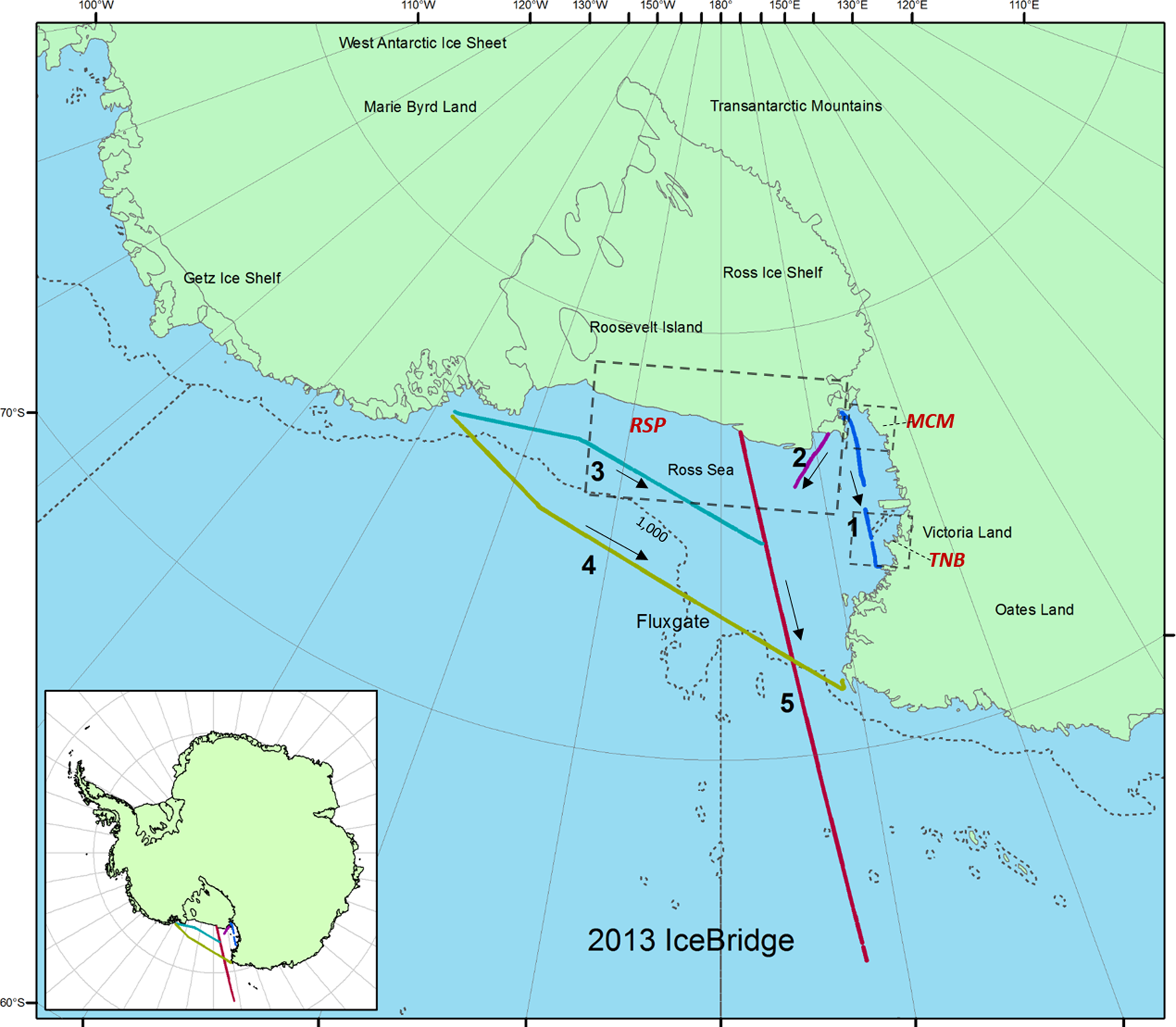
Fig. 1. IceBridge flights (#III and #VI) in the Ross Sea, Antarctica on 20 and 27 November 2013, respectively, with tracks 1, 2, 3, 4 for flight #III and track 5 for flight #VI. Track 4 is the line identified as the Ross Sea fluxgate roughly over the 1000 m bathymetry contour separating the continental shelf to the south from the deep ocean to the north. The arrows show the direction of each track that is used for data analysis and discussion purposes only. The three polynyas are Ross Ice Shelf polynya (RSP), Terra Nova Bay polynya (TNB) and McMurdo Sound polynya (MCM).
The objectives of this study are to (1) compute total freeboard and ice thickness using the data collected from 2013 NASA Operation IceBridge (OIB) airborne overflights in the Ross Sea, (2) examine the distribution of freeboard and ice thickness over the Ross Sea, and (3) compare our results of OIB (2013) with an ICESat freeboard product (2003–2008).
2. Data and methods
2.1 OIB datasets
NASA's OIB mission flew over the Ross Sea, Antarctica (20 and 27 November 2013) and collected important surface sea-ice data with Airborne Topographic Mapper (ATM) and Digital Mapping System (DMS) instrumentation for the first time.
ATM data are the surface elevation data acquired through an airborne Light Detection and Ranging (LIDAR) system using a scanning laser beam (Krabill, Reference Krabill2013). The ATM is a 532 nm wavelength conically scanning laser altimeter with a pulse repetition frequency of 5 kHz and an off-nadir scan angle of ~15° (T2 scanner) or 23° (T3 scanner), combined with a differential GPS system for aircraft positioning and an inertial navigation system to measure aircraft orientation. The footprint size of each individual elevation measurement is ~1 m, which is set by the laser beam divergence. The ATM data are referenced to the ITRF-2005 reference frame and projected onto the WGS-84 ellipsoid (Krabill, Reference Krabill2013; Kurtz and others, Reference Kurtz2013; Wang and others, Reference Wang, Xie, Ke, Ackley and Liu2013). Two types of ATM data sets with different resolution are analyzed in this study, ATM L1B (~1 m) and L2 (80 m sample width by ~60 m along track). The L1B data are the ATM Level-1B Qfit Elevation and Return Strength data with all biases and offsets including heading, pitch, roll, ATM-GPS offset, scanner angles, range bias removed. Each surface elevation measurement corresponds to one laser pulse. The measurements have not been resampled. Nominal spatial resolution is 1 m (Krabill, Reference Krabill2013). The L2 data are the ATM Level-2 Ice Elevation, Slope and Roughness data sets that are re-sampled and averaged from ATM L1B data. The L2 elevation measurements have been resampled at the distance interval along the flight track of ~60 m, which is controlled by aircraft speed. Each set of along-track records contains a fixed 80 m across-track nadir platelet as well as three or five additional platelets that together span the entire swath of the ATM scan (Wang and others, Reference Wang, Xie, Ke, Ackley and Liu2013; Studinger, Reference Studinger2016). L1B data are used to calculate local sea level over leads identified using DMS imagery, while L2 data are used for total freeboard retrieval in this paper.
DMS data, high-resolution natural color and panchromatic imagery, have a pixel resolution from 0.015 to 2.5 m depending on flight altitude (0.1 m at an altitude of 457 m), also is referenced to the WGS84 ellipsoid (Dominguez, Reference Dominguez2010).
2.2 ICESat freeboards
In 2003, ICESat was launched by NASA with a Geoscience Laser Altimeter System (GLAS) for measuring surface elevations (Zwally and others, Reference Zwally2002). It sampled the Earth's surface from an orbit with inclination of 94° with footprints of ~70 m in diameter spaced at ~170 m intervals (Kwok and others, Reference Kwok, Zwally and Yi2004). The 2003–2008 ICESat freeboard data, which were derived by using a local sea level reference obtained by the lowest (2%) elevation values within a 50 km section (Kern and Spreen, Reference Kern and Spreen2015), are used in this study. In order for ICESat data to have enough footprints to do statistics and for comparison with IceBridge data, the full spring seasons (see Table 2 of Li and others, Reference Li2018) of ICESat data are used. A buffer zone within a distance of 30 km at each side of each IceBridge track is used to extract the ICESat freeboard values. This allows an approximate colocation of the ICESat and IceBridge data.
2.3 Mean Sea Surface data
The DTU15 Mean Sea Surface Height (MSSH) is used as a geoidal sea level reference to do the geoid correction of ATM L1B and L2. The DTU15 Mean Sea Surface (MSS) released from DTU (Technical University of Denmark) is a global, high-resolution mean sea surface with a resolution of 1 min by 1 min. This is based on the DTU13 model through the usage of multi-mission satellite altimetry gathered from ten different satellites (Andersen and others, Reference Andersen, Knudsen and Stenseng2015). Merging of Cryosat-2 LRM, SAR and SAR interferometry (SAR-In) data and the down-weighting of ICESat data are significant recent advances that provide greater advantages over previous MSS estimates (Andersen and others, Reference Andersen, Stenseng, Piccioni and Knudsen2016; Skourup and others, Reference Skourup2017). The averaging period of this MSS is 1993–2012. The MSS is the sum of geoid and ocean mean dynamic topography (Andersen and others, Reference Andersen, Stenseng, Piccioni and Knudsen2016).
2.4 Lead detection and sea-ice thickness retrieval methods
To calculate total freeboard, an instantaneous local Sea Surface Height (SSH) reference must be determined first (Kurtz and others, Reference Kurtz2009; Xie and others, Reference Xie, Tekeli, Ackley, Yi and Zwally2013). The key location used to obtain SSH is through the identification of leads (open water or very thin ice) (Xie and others, Reference Xie, Tekeli, Ackley, Yi and Zwally2013; Wang and others, Reference Wang, Guan, Liu, Xie and Ackley2016). There are four main methods used to obtain SSH. The first is to take a percentage of lowest-elevation points along a range distance of a flight track, and calculate the average height of these points (Zwally and others, Reference Zwally, Yi, Kwok and Zhao2008). We call this ‘the lowest elevation method’ in this study. The second and third methods are to identify leads/water either by the apparent reflectivity of the transmitted laser pulse (Kwok and others, Reference Kwok, Cunningham, Manizade and Krabill2012) or by the waveform characteristics of radar altimetry data (Farrell and others, Reference Farrell, Laxon, McAdoo, Yi and Zwally2009). The apparent reflectivity is defined as the ratio of the reflected laser signal strength to the transmitted signal strength (Wang and others, Reference Wang, Guan, Liu, Xie and Ackley2016). Leads have low apparent reflectivity. The raw data of radar altimetry satellite are recorded as a waveform (power in y-axis and gate number in x-axis) (Nababan and others, Reference Nababan, Hakim and Panjaitan2018). Echo waveforms from lead footprints have one single peak with high echo power (Xia and Xie, Reference Xia and Xie2018). These three methods, used with satellite altimetry data, have limitations due to the paucity of optical images to verify results. The fourth method, only available from airborne data, is to use optical images that are collected simultaneously with the laser altimetry data to visually identify leads and their average height of the laser shots within leads is then taken as the lead surface height (Kurtz and others, Reference Kurtz2013; Onana and others, Reference Onana2013; Wang and others, Reference Wang, Xie, Ke, Ackley and Liu2013; Wang and others, Reference Wang, Guan, Liu, Xie and Ackley2016). Since the reflectivity of laser shots on thick sea ice is much higher than on leads (Kwok and others, Reference Kwok, Cunningham, Manizade and Krabill2012), reflectivity values can be used to exclude misclassified leads (Wang and others, Reference Wang, Guan, Liu, Xie and Ackley2016).
In this study, we combine the DMS-mapped leads and L1B laser shots on leads to get the most realistic local sea levels, then apply to L2 data for freeboard retrieval, as our objective method. We also apply the lowest (2%) elevation method to provide a reference for later evaluation, in order to compare with satellite altimetry from ICESat. We compare the total freeboard derived from these two methods to evaluate how each method affects the results.
Total freeboard can be converted to ice thickness through different approaches: buoyancy equation method (Zwally and others, Reference Zwally, Yi, Kwok and Zhao2008; Weissling and others, Reference Weissling, Lewis and Ackley2011), zero sea-ice freeboard assumption method (Kurtz and Markus, Reference Kurtz and Markus2012) and empirical equation method (Xie and others, Reference Xie2011; Ozsoy-Cicek and others, Reference Ozsoy-Cicek, Ackley, Xie, Yi and Zwally2013; Li and others, Reference Li2018). For the buoyancy equation, accurate estimates of snow depth and densities of snow, sea ice and seawater are essential for deriving an accurate estimate of ice thickness (Zwally and others, Reference Zwally, Yi, Kwok and Zhao2008; Weissling and others, Reference Weissling, Lewis and Ackley2011). The major limitation of using a buoyancy equation in Antarctica is the uncertainty of snow depth retrieval (Markus and Cavalieri, Reference Markus and Cavalieri1998). In this 2013 Ross Sea campaign, snow depth data through the snow radar is not available, and therefore, the buoyancy equation is not feasible. From both approaches of zero sea-ice freeboard assumption and empirical equation, however, sea-ice thickness can be directly estimated from total freeboard without knowing snow depth. The zero sea-ice freeboard assumption approach assumes that snow depth is equal to the total freeboard (Kurtz and Markus, Reference Kurtz and Markus2012), which is not always true, particularly for thinner ice with no snow cover at all. This could result in an underestimate of sea-ice thickness (Kwok & Kacimi, Reference Kwok and Kacimi2018; Kern and others, Reference Kern, Ozsoy-Çiçek and Worby2016). The empirical equation approach provides a direct conversion of total freeboard into sea-ice thickness, totally based on field measurements. For this Ross Sea case, the empirical linear equation between ice thickness and total freeboard was derived from the measurements of 23 profiles (of 50–100 m in length each) during the NB Palmer September/October 1994 cruise (Jeffries and others, Reference Jeffries, Li, Jana, Krouse, Hurst-Cushing and Jeffries1998; Ozsoy-Cicek and others, Reference Ozsoy-Cicek, Ackley, Xie, Yi and Zwally2013) and is used for this study. Based on their study (Ozsoy-Cicek and others, Reference Ozsoy-Cicek, Ackley, Xie, Yi and Zwally2013), the R2 of the empirical equation is 0.83, meaning this linear equation could explain 83% of the measured ice thickness variation.
2.5 Objective method
A flow diagram of the objective method using DMS and L1B with the laser shots reflectivity to identify leads is shown in Figure 2 and a description of each step is given below.

Fig. 2. Workflow chart for deriving total freeboard and ice thickness from IceBridge ATM and DMS data. SSH, sea surface height; MSSH, mean sea surface height; SSHA, sea surface height anomaly.
2.5.1 DMS classification
Leads are optically dark features with low reflected pixel intensities (DN values) while snow/sea ice have high reflected pixel intensities in high-resolution natural color DMS photographs. The distribution of pixel intensities thus provides a practical way to separate leads from sea ice (Onana and others, Reference Onana2013; Wang and others, Reference Wang, Guan, Liu, Xie and Ackley2016). Wang and others (Reference Wang, Guan, Liu, Xie and Ackley2016) found that the pixel intensities of leads and snow/thick sea-ice surface had two distinguishable modes and can be used to develop dynamic pixel intensity thresholds to do the classification. As the pixel intensities of snow/sea ice are determined by the solar illumination and vary with the Sun elevation and weather conditions, dynamic thresholds varying from image to image, instead of a fixed threshold for all images, are used in this study to detect the leads. We use this principle to manually select all the images with the leads first and then automatically detect the first mode value (mode of leads) image by image to do the classification. The lead class is then transformed into a shapefile and used as a mask (Fig. 2).
2.5.2 ATM L1b and ATM L2 preprocessing
Both ATM L1B and L2 data are processed into shapefile data. Because the reflectivity of laser shots on thick sea ice is much higher than on leads, the reflectivity value (R) of 0.25 (Kwok and others, Reference Kwok, Cunningham, Manizade and Krabill2012) is set as the threshold of L1B data to extract lead shots, i.e., R < 0.25 as leads. Misclassified leads are then excluded by using the DMS-derived lead mask. By combining DMS images (leads mask) and the reflectivity of ATM L1B, sea surface shots within leads are determined. Shots of both L1B and L2 are then processed with geoid correction by subtracting DTU 15 MSSH (Fig. 2). We then use ATM L2 to calculate total freeboard. In this study, we use Sea Surface Height Anomaly (SSHA) instead of SSH.
2.5.3 Computation of SSHA
After sea surface shots of one lead are detected, the elevation average after geoid correction (i.e., SSH-MSSH) is computed as SSHA of this lead. Shots falling outside one std dev. are treated as outliers and deleted. Weighted inverse distance interpolation is used to predict the SSHA at locations without leads present. The SSHA profile along each flight track is then obtained.
2.5.4 Computation of freeboard and ice thickness
Total freeboard (F) is calculated by using the surface elevation of ATM L2 minus the corresponding DTU 15 MSSH and SSHA. Ice thickness is then retrieved from total freeboard by an empirical equation (Ozsoy-Cicek and others, Reference Ozsoy-Cicek, Ackley, Xie, Yi and Zwally2013), derived from ice thickness and freeboard surveys in the Ross Sea region:

2.6 The lowest elevation method
When optical images are not available concurrently with satellite altimetry, previous researchers have used a percentage of the lowest-elevation points along a flight track range, and then calculated the average height of these points as the local sea level (Zwally and others, Reference Zwally, Yi, Kwok and Zhao2008). When using the lowest elevation method, another key factor is the length of the section that is chosen to determine the local sea level. Since previous studies used both 25 and 50 km sections in processing ICESat data (Zwally and others, Reference Zwally, Yi, Kwok and Zhao2008; Kern and Spreen, Reference Kern and Spreen2015), these two section lengths have thus been used in this study for comparison.
3. Results
3.1 Sea Surface Height Anomaly
Figure 3 shows lead SSHA for all tracks. Track 5 has the highest SSHA with the largest std dev. The std dev. quantifies how close the shot SSHA values are to the mean value. Once the shot SSHA value exceeds one std dev. away from the mean value, we treat it as an outlier. These outliers can be either indicative of thicker ice or reflection beneath the water surface and are not representative of the true sea level.

Fig. 3. Local sea surface height anomaly (SSHA, black) with ±1 std dev. (red), along the distance direction (start and end) as indicated in Figure 1.
3.2 Distribution of freeboard and ice thickness in the Ross Sea
The total freeboard and ice thickness distributions along the five Ross Sea tracks are shown in Figures 4 and 5. Both tracks 1 and 2 show evidence of very thick ice, likely caused by thick ice proximity to the coastal area.

Fig. 4. Total freeboard (top panels, gray) and derived ice thickness (bottom panels, red) as a function of distance along each track.

Fig. 5. Spatial distribution of freeboard along each track (center) with a zoom-in window showing the ATM L2 shots on DMS imagery (track 3, 4 and 5) and MODIS imagery (tracks 1 and 2) for sampled ice types on different tracks. Tracks 1 and 2 had an apparent abrupt increasing freeboard (ice thickness) toward the Ross Island (see the zoom-in windows 1 and 2) with freeboard exceeding 1 m. The MODIS true color image was on 20 November 2013, the same day as the tracks 1 and 2.
Along tracks 3 and 4 (Figs 4 and 5), thick ice is evidenced along the east section of track 3 and the east and the far west sections of track 4. These thickened ice locations could be attributed to older ice on the east and ridged ice elsewhere. The majority of the ice, however, is thin ice with a modal value of 0.35 m for track 3 and 0.45 m for track 4 (Fig. 6), thinner southwards and thicker northwards. Track 4 was designed to follow the fluxgate (Fig. 5), separating the continental shelf region to the south from the deep ocean to the north, where ice produced from the coastal polynyas is exported. It is clear that the ice is relatively thinner in the middle section of the fluxgate in comparison to the west and east sections (Fig. 4). This is evidence of ice produced in coastal polynyas (RSP, TNB and McMurdo Sounds polynya) which is pushed northwards due to katabatic winds off the continent (Parish, Reference Parish1988) with the ice becoming thicker as it grows with age as it moves away from the polynyas. This phenomenon is best supported by the thickness distribution along track 5, starting from the RSP and ending north 1400 km away, with two peaks of modal thickness: 0.35 m to the south and 0.7 m to the north (Figs 4–6).

Fig. 6. Frequency distributions of freeboard (top panels, gray) and ice thickness (bottom panels, red) with mean, std dev. (SD), mode and total count number for each track.
The histograms of freeboard and thickness along tracks 1 and 2 (Fig. 6) include three modes for freeboard: 0.05, 0.55 and 1.05 m (track1) and 0.05, 0.40 and 1.10 m (track 2); and for ice thickness: 0.35, 1.55 and 2.75 m (track 1) and 0.35, 1.20 and 2.90 m (track 2). The first mode represents the new and young ice in the region and it is the dominant ice type. This is mostly produced in the polynyas due to the katabatic winds continuously pushing new ice away and ice forming in the open water behind it. As the ice drifts northwards, it thickens thermodynamically with age. The third mode indicates the thickest and ridged ice, although amounting to only a small portion of the ice along the two tracks. For example, the thickest ice of tracks 1 (up to 3 m) and 2 (up to 5 m) is very close to the Ross Island where thick fast ice develop (Fig. 5).
3.3 Comparison of OIB total freeboard from different methods
Figures 7 and 8 show that the results from this method which detects leads by combining DMS images and reflectivity of ATM L1B and the method used the lowest 2% elevation at 25 or 50 km range (Figs 7 and 8). The track 5 from this study has two clear modes rather than one single mode from the lowest elevation method (Fig. 7). Interestingly, the mean values estimated from both methods are nearly the same (Fig. 8). This comparison indicates that lowest elevation method may overestimate the freeboard and not be able to differentiate the thin ice types from in the distribution of freeboards (>6 cm), but mean values of the distribution are affected less (<9 cm).

Fig. 7. Kernel density distributions of freeboard (from IceBridge 2013 Ross Sea data) with different methods: using DMS images and ATM derived local sea level (red, objective method in this study), the lowest 2% elevations of 25 km along track as local sea level (blue), and the lowest 2% elevations of 50 km along track as local sea level (green). Kernel density estimation (KDE) is a widely used non-parametric way to estimate the probability density function of a random variable, and it is a smoothing technique to visualize the discrete histogram (Duong, Reference Duong2007).

Fig. 8. Mean (m) and principal (most frequent) modal value (m) of freeboard (from IceBridge 2013 Ross Sea data), with a, b and *, respectively, referring to the 50 km, 25 km lowest (2%) elevation methods, and the objective method combined with ATM and DMS as described in Figure 7.
Although similar patterns in the distributions (Figs 7 and 8), the 25 km section method results in lower freeboards than the 50 km section method and it is closer to the freeboard mean values (within 5 cm) derived from our objective method.
3.4 Comparison of OIB (2013 a) with ICESat (2003–2008)
The 2003–2008 ICESat freeboard used in this paper was derived from the lowest 2% elevation of 50 km section method (Kern and Spreen, Reference Kern and Spreen2015) and can be compared with the 2013 OIB freeboard from the lowest (2%) elevation method with 50 km section (2013 a) to examine the interannual differences. Mixed results are found, with no clear trend from the ICESat 2003–2008 era to 2013 (Fig. 9). In terms of mean ice thickness (Fig. 10), there is a clear increase along the two short tracks (1 and 2) but no change or slight decrease for ice along the other three long tracks. Track 5 is the most stable track, and does not have much change from 2003 to 2013 (Figs 9 and 10). In general, the ice thickness in 2006 and 2007 was thicker (Figs 9, 10 and 12).

Fig. 9. Kernel density distributions of freeboard (from IceBridge 2013 Ross Sea data) based on the lowest 2% elevations of 50 km along track as local sea level and 2003–2008 ICESat total freeboard using the same method (2% with 50 km).

Fig. 10. Mean (m) and modal value (m) of total freeboard from ICESat (2003–2008) and ATM (2013 a, here ‘a’ refers to 50 km lowest 2% elevation as described in Fig. 7).
4. Discussion
Although the mean reflectivity values of leads for all 2013 IceBridge tracks in the Ross Sea are <0.25, it is found that the reflectivity could change with a few gaps even in one track (Fig. 11). For tracks 2 and 5, most reflectance values are 0.15 or below, indicating it could overestimate the amount of leads if a single threshold value of 0.25 is used for separating leads from thick ice as done in Kwok and others (Reference Kwok, Cunningham, Manizade and Krabill2012). The major reason for such variances may be due to weather conditions and the difference in solar elevation angles along tracks, though the surface reflectance itself does not change, unless the surface changes. Therefore, to get an accurate separation of leads from thick ice, a section by section or time by time determination of the lead reflectance is required.

Fig. 11. Mean reflectance (blue) of all L1B shots within leads along the five tracks, with the distance direction (start and end) as indicated in Figure 1.
Wang and others (Reference Wang, Guan, Liu, Xie and Ackley2016) found that, within a 45 km section of one ATM L1B track, the SSH demonstrates a linear gradient, which is applied to derive SSHs where there are no leads. In this study, a similar linear gradient of the SSHA was found within a 45 km section, but with several fluctuations along the whole track (Fig. 3). So, considering the entire long track, the Inverse Distance Weighting method is a better method to interpolate the SSHA for the locations without leads, by using a linear combination of values at sampled points weighted by an inverse function of the distance from the point of interest to the sampled points (Li and Heap, Reference Li and Heap2008).
In this paper, we use the empirical equation to calculate sea-ice thickness. The equation was derived from in situ measurements on Ross Sea taken by Palmer September and October 1994 cruise (Ozsoy-Cicek and others, Reference Ozsoy-Cicek, Ackley, Xie, Yi and Zwally2013). Kern and others (Reference Kern, Ozsoy-Çiçek and Worby2016) inter-compared different methods to retrieve sea-ice thickness, including empirical equation, equation with zero sea-ice freeboard assumption (Kurtz and Markus, Reference Kurtz and Markus2012) and the physically-based method with snow depth as an input. They found common to all approaches is the thin sea-ice thickness of 1–2 m in the Ross Sea downstream of the RSP (Figs 2, 5, Kern and others, Reference Kern, Ozsoy-Çiçek and Worby2016). Further, values derived from empirical equations are higher than those from the zero sea-ice freeboard assumption approach but lower than those from the physically-based method. The sea-ice thickness around the fluxgate could be 1 m lower than the physically-based method (Fig. 5, Kern and others, Reference Kern, Ozsoy-Çiçek and Worby2016). Considering the complexity of snow depth in the Ross Sea and the limitation of field measurements, a thorough analysis of uncertainties is hard to make. The scientific cooperation and data sharing could provide effective ways to develop the methods of thickness retrieval in the near future.
The objective method combining the use of the DMS and L1B can provide a more accurate local sea level for deriving total freeboard in comparison to the lowest elevation method which only uses elevation data. The results of this study provide a reference to evaluate the lowest elevation method. It is found that the lowest elevation method overestimates the freeboard, especially the lowest peak of freeboard distribution. It also indicates that the mean values are less affected than mode values, because spatial aliasing on sea-ice thickness raises the mode value impact but affects the mean less (Geiger and others, Reference Geiger, Müller, Samluk, Bernstein and Richter-Menge2015). High-resolution optical imagery, however, is not always available, for example, for ICESat and ICESat-2. Using a better method to derive local sea level from ICESat-2 is very important (Markus and others, Reference Markus2017) and requires further study. The results also show the freeboard from 25 km range method is closer to our results than the 50 km range derived freeboard. This could provide a reference to researchers on determining the optimal distance-section when using the lowest elevation method.
Using the same method when comparing the ICESat freeboard with the 2013 OIB freeboard (2013 a) results is in no clear trend in the time ranging from the ICESat era to 2013, although some year-to-year variability is observed. This comparison has two limitations as different date period and location of the tracks (Fig. 12) are used when this comparison is made. To gather adequate ICESat statistical evidence, the spring seasons (see Table 2 of Li and others, Reference Li2018) of ICESat data are included, and a buffer zone within 30 km of each side for each IceBridge track is used to extract the ICESat freeboard values (Fig. 12). We expect that the ICESat-2 provides much more effective footprints due to its six beams, 17 m footprint and the 0.7 m intervals along track.

Fig. 12. Spatial distribution of total freeboard for each track from ICESat (2003–2008) and ATM (2013 a, 2013 b and 2013 *). Letters ‘a’, ‘b’ and symbol ‘*’ following 2013 refer to the different methods used as in Figure 7. The gray circle represents the area with the lowest freeboard (the thinnest ice).
Figure 12 shows the freeboard spatial distribution of ICESat 2003–2008 and 2013 OIB with three different methods. It indicates a similar distribution pattern, being thinner in the center part (gray circle), and thicker in the east, north or near coastal (but not the polynyas). This supports the hypothesis that ice produced in coastal polynyas (i.e., Ross Ice Shelf, Terra Nova Bay and McMurdo Sound) is pushed away to the north due to katabatic winds off the continent (Parish, Reference Parish1988) and the ice thickens as it ages and is deformed further away from the polynyas. It also indicates all these methods can provide a relatively good spatial distribution to a certain degree, though some differences in absolute values.
Calculation of the exported ice volume from the Ross Sea polynyas depends on the ice thickness. Area flux can be converted to volume flux by multiplying the area by ice thickness measurements. Most researchers (Kwok, Reference Kwok2005; Martin and others, Reference Martin, Drucker and Kwok2007; Comiso and others, Reference Comiso, Kwok, Martin and Gordon2011; Drucker and others, Reference Drucker, Martin and Kwok2011) use an average of the ice thicknesses measured by Jeffries and Adolphs (Reference Jeffries and Adolphs1997) from shipboard inside the fluxgate in the western Ross Sea during May–June 1995, where they found an average thickness of 0.66 ± 0.33 m. However, this estimate neglects the space/time variability in sea-ice thickness as well as the thicker multiyear ice fraction. Year to year variations in mean thickness would change the total volume exported, independent of the net areal export. Track 4 was designed to follow the fluxgate through which newly produced ice from the coastal polynyas is exported. Table 1 shows a comparison of mean sea-ice thickness values along the fluxgate by this research and shipboard. It indicates that mean ice thickness estimates experienced great change from 1995 to 2013. Comiso and others (Reference Comiso, Kwok, Martin and Gordon2011) estimated that the positive rate of increase in the net ice area export is ~30 000 km2 a−1 over the Ross Sea Shelf from 1992 to 2008 and the corresponding volume transport is ~20 km3 a−1 (similar to Drucker and others, Reference Drucker, Martin and Kwok2011) using a 1995 shipboard mean ice thickness of 0.6 m. ICESat data provided a mean sea-ice thickness of 0.93 m from 2003 to 2008 (Table 1), which indicated a much larger volume transport over 2003–2008 than 2013 ATM with optical images that show a mean thickness of only 0.48 m (Table 1), which gives a more precise value for recent year's volume transport estimation. Kwok and others (Reference Kwok, Pang and Kacimi2017) examined mean exportable sea ice at the fluxgate as 750 × 103 km2 in the past 33 years, with an increase of 7.7 × 10³ km2 a−1 from 1982 to 2015. These thickness values could then help to give an estimation of exported ice volume at the fluxgate (Table 1). Using mean thickness values along track 4 from both ICESat and ATM exported ice volume at the flux gates is estimated as higher for the ICESat years (2003–2008) than for the IceBridge year (2013) (Table 1). Track 5 starts from the RSP and ends north 1400 km away, the ice thickness is clearly thinner than that northwards from the fluxgate with a clear two peaks of modal thickness: 0.35 m to the south and 0.7 m to the north (Figs 4–6). This can provide a correct estimate of the ice volume over the continental shelf. Knowing thickness distribution is critical for estimating the volume export and will help researchers to better specify SIP in the Ross Sea. The implications for the formation of dense shelf water and its recent changes by SIP can then be calculated more accurately, developing a better understanding of the observed freshening in the Ross Sea (Jacobs and Giulivi, Reference Jacobs and Giulivi2010). Differentiating the ice thickness north and south of the fluxgate is important for obtaining an accurate estimate of the ice volume over the continental shelf.
Table 1. Comparison of mean sea-ice thickness values along the fluxgate and estimation of exported ice volume based on area export data from Kwok and others (Reference Kwok, Pang and Kacimi2017)

The 1995 measurements are shipboard data inside the fluxgate in the western Ross Sea during May–June 1995 (Jeffries and Adolphs, Reference Jeffries and Adolphs1997). Letters ‘a’, ‘b’ and symbol ‘*’ refer to the different methods used as in Figure 7.
5. Conclusions
In this study, leads are detected by combining DMS images and reflectivity of ATM L1B, and local sea level are retrieved from ATM L1B shots over leads. Freeboard estimates are obtained from the difference between surface elevation of ATM L2 and the local sea level. Finally, total freeboard is converted to ice thickness through an empirical equation, which does not require knowledge of the snow depth. The OIB 2013 data in the Ross Sea are examined. The results show the dominant ice thickness modal values of all tracks are between 0.35 and 0.45 m, with mean ice thickness values between 0.48 and 0.99 m. The sea-ice thickness along track 5, starting in the RSP and ending 1400 km to the north, is clearly thinner to the south than to the north of the fluxgate with two well-defined modal thickness peaks: 0.35 m to the south and 0.7 m to the north. This is evidence that the ice produced in coastal polynyas when transported from the shelf northwards by katabatic winds becomes thicker as it grows in age and deformation away from the polynyas. This phenomenon is also supported by tracks 3 and 4. Track 4 was designed to follow the fluxgate, which separates the continental shelf from the deep ocean, and track 3 is further south parallel to track 4. The sea ice in track 4 is thicker than that in track 3 with modal values of 0.45 m for track 4 and 0.35 m for track 3. The ice of track 4 is relatively thinner in the middle section of the fluxgate than that in the west and east sections of the fluxgate.
In addition, the lowest 2% elevation method is applied to the IceBridge airborne data previously used with ICESat satellite data to derive total freeboard. It is found that the lowest elevation method could overestimate the freeboard. When comparing the ICESat freeboard with the 2013 OIB freeboard (2013 a) by using the same method, large interannual variability is observed, with no clear increase or decrease from the 2003–2008 ICESat era to 2013. This comparison, however, is limited by the fact that the locations and time periods of the tracks are not exactly the same.
Spatial distributions of freeboard, ICESat 2003–2008 and 2013 OIB with different methods, have a similar pattern, thinner in the center part (gray circle), and thicker in the east, north or more near coasts (but away from the polynyas). Though different methods have differences in absolute values, they are still able to reflect the same spatial distribution pattern, which suggests that the mean sea-ice thickness values are less affected by different methods and datasets. Comparison of mean sea-ice thickness values along the fluxgate, such as the one presented in this study could help provide a more accurate estimate of the ice volume over the continental shelf and thus better estimate SIP in the Ross Sea. Further examination and verification are forthcoming using ICESat-2 data as well as 2016 and 2017 airborne flights using the IcePod system (ATM and DMS) on NSF's C-130 aircraft.
Acknowledgements
We acknowledge the funding supports from the US National Science Foundation (NSF) Award (#134717) (S.F. Ackley and H. Xie, PIs) and NASA Award (#80NSSC19M0194) (H. Xie, A.M. Mestas-Nuñez and S.F. Ackley, PIs). We also acknowledge all the researchers and institutions that have shared the datasets in which this study is based (available at https://nsidc.org/icebridge/portal/map, ftp://ftp.space.dtu.dk/pub/DTU15/), and Stefan Kern at the University of Hamburg for the ICESat freeboard data.


 Open access