


INTRODUCTION
Polar ice sheets play an important role in the global climate system. Their significance means we must be able to measure and monitor their status in order to understand and predict their future evolution and stability (Budd and Jacka, Reference Budd and Jacka1989; Alley and others, Reference Alley, Clark, Huybrechts and Joughin2005). Since the 1950s, Radio Echo Sounding (RES, also known as ice-penetrating radar – IPR) has been widely used in ice-sheet exploration to great success due to its high precision and efficiency (compared with seismic sounding, which yields similarly accurate results, RES mounted on aircraft can increase the rate of data acquisition by 5 orders of magnitude) (Robin and others, Reference Robin, Evans and Bailey1969; Clough, Reference Clough1977). RES provides not only direct geometrical parameters such as thickness and subglacial topography, but also internal ice-sheet characteristics such as internal layers and structures, and subglacial conditions, which collectively make it perhaps the most powerful technique used in field glaciology (Siegert and others, Reference Siegert2004; Eisen and others, Reference Eisen, Hamann, Kipfstuhl, Steinhage and Wilhelms2007; Bingham and others, Reference Bingham2012).
The application of airborne synthetic aperture radar (SAR) in glaciology can be dated back to an experiment in Greenland in 1999 (Gogineni and others, Reference Gogineni2001). In this exercise, SAR results were achieved by the coherent stacking of sequential multiple small-sized apertures, so improving the image resolution and making it a standard for processed airborne RES (Legarsky and others, Reference Legarsky, Gogineni and Akins2001; Peters and others, Reference Peters, Blankenship and Morse2001, Reference Peters2007; Heliere and others, Reference Heliere, Corr and Lin2006). Despite this notable advance, during data collection received signals are often inevitably mixed with interference, which leads to ‘strip noise’ in the RES record. While strip noise is not too obvious when the signal-noise-ratio of the radio-echo is high, such as from shallow layers in the ice, when the echo from deep regions of ice sheet becomes faint strip noise becomes a serious impedance to data quality. Such noise leads to problems in interpreting ice thickness, basal echo-free zones (EFZs) and subglacial conditions (such as bed roughness, and frozen vs wet beds).
Strip noise can be categorized into three types: horizontal, vertical and inclined (diagonal) stripes. Horizontal stripes in RES data can come from crystal oscillator noise, thermal drift of electronic elements, multiple reflections or the first arrival air wave. Vertical strips are caused by physical irregularities in the propagating media, instrument instability in time and bursts of electromagnetic pulse interference. Inclined strips are commonly seen in near-surface records as ‘X-shaped’ interference patterns, caused by surface reflections from buildings and other large metal objects.
In remote sensing, strip noise removal is a topic of high interest and many methods have been proposed, including: (1) moving average filtering (Cai, Reference Cai2004; Boin and Haibel, Reference Boin and Haibel2006); (2) histogram matching (Rakwatin and others, Reference Rakwatin, Takeuchi and Yasuoka2007); (3) interpolation approaches (Tsai and others, Reference Tsai, Lin, Rau, Chen and Liu2005); (4) frequency filtering with Fast Fourier Transforms (FFT) (Liu and Morgan, Reference Liu and Morgan2006; Arrell and others, Reference Arrell, Wise, Wood and Donoghue2007); and (5) wavelets analysis (Pande-Chhetri and Abd-Elrahman, Reference Pande-Chhetri and Abd-Elrahman2001; Tang and others, Reference Tang, Ning, Yu and Conover2001; Torres and Infante, Reference Torres and Infante2001; Chen and others, Reference Chen, Lin, Shao and Yang2006; Münch and others, Reference Münch, Trtik, Marone and Stampanoni2009). While a few research studies have focused on de-striping using filtering (Swenson and Wahr, Reference Swenson and Wahr2006; Li and Shen, Reference Li and Shen2011; Wilken and others, Reference Wilken, Feldens, Wunderlich and Heinrich2012; Horsley and others, Reference Horsley, Wright and Barrier2014; Shaaban and others, Reference Shaaban2014 ), it has been shown to be problematic because insufficient filtering leads to the strip noise remaining, and over-filtering leads to signal loss or signal distortion (Zhang, and others, Reference Zhang, Zhang, Yu and Pan2010; Bao, and others, Reference Bao, Li and Chen2014; Wang, and Liu, Reference Wang and Liu2017).
Here, we present a method for removing strip noise in RES data using wavelet decomposition and two-dimensional discrete Fourier transform (2-D DFT) filtering. The 2-D DFT spectrum of the strip noise keeps its linear features in wavelet components at all levels, so we can apply appropriate Gaussian filtering on the necessary coefficients at scales necessary to remove the linear strip frequency spectrum with less impact on the effective signal. Then, inverse wavelet transform restores the remaining parts to yield a de-stripped product. This de-striping method has few limitations or requirements, and can be used in other geophysical techniques where strip removal is advantageous.
METHOD
Snow Eagle IPR
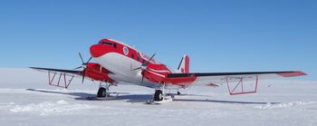
The Chinese Antarctic research expedition (CHINARE) recently configured a polar airborne geophysical platform, Snow Eagle 601, which is capable of gravity, magnetic, RES, GPS, optical and laser surface altimetry measurements (Fig. 1). In the 32nd CHINARE expedition (2015/16), Snow Eagle accomplished 18 flights of geophysical survey covering the previously uncharted region of Princess Elizabeth Land in East Antarctica. The RES system on Snow Eagle (the ‘Snow Eagle IPR’; Cui and others, Reference Cui2018) is a coherent RES instrument functionally similar to the High Capability Radar Sounder (HiCARS) developed by the University of Texas Institute for Geophysics (UTIG), which has been used on several platforms and projects (e.g., Young and others, Reference Young2011; Greenbaum and others, Reference Greenbaum2015) (Fig. 2). The Snow Eagle IPR's transmitting signal is a 1 µs chirp pulse, with a 60 MHz center frequency (3 m wavelength in the ice) and a 15 MHz bandwidth. The vertical resolution of ice penetrating radar systems is related to the signal source wavelet, the receiver bandwidth, the sampling rate, the processing applied and the medium through which the signal transmits; the Snow Eagle IPR has a fundamental vertical resolution of approximately 5.6 meters in ice (Cavitte and others, Reference Cavitte2016). The transmitted signal is generated digitally by a National Instruments PXI controller with samples frequency of 200 MHz, fed into an 8 kW Tomco amplifier. The pulse repetition frequency is 6250 Hz, with 32 stacking traces, a record length of 64 µs, ‘slow time’ sampling at 196 Hz, a typical Doppler frequency of 36 Hz and a dynamic range of 120 dB (Peters and others, Reference Peters2007).
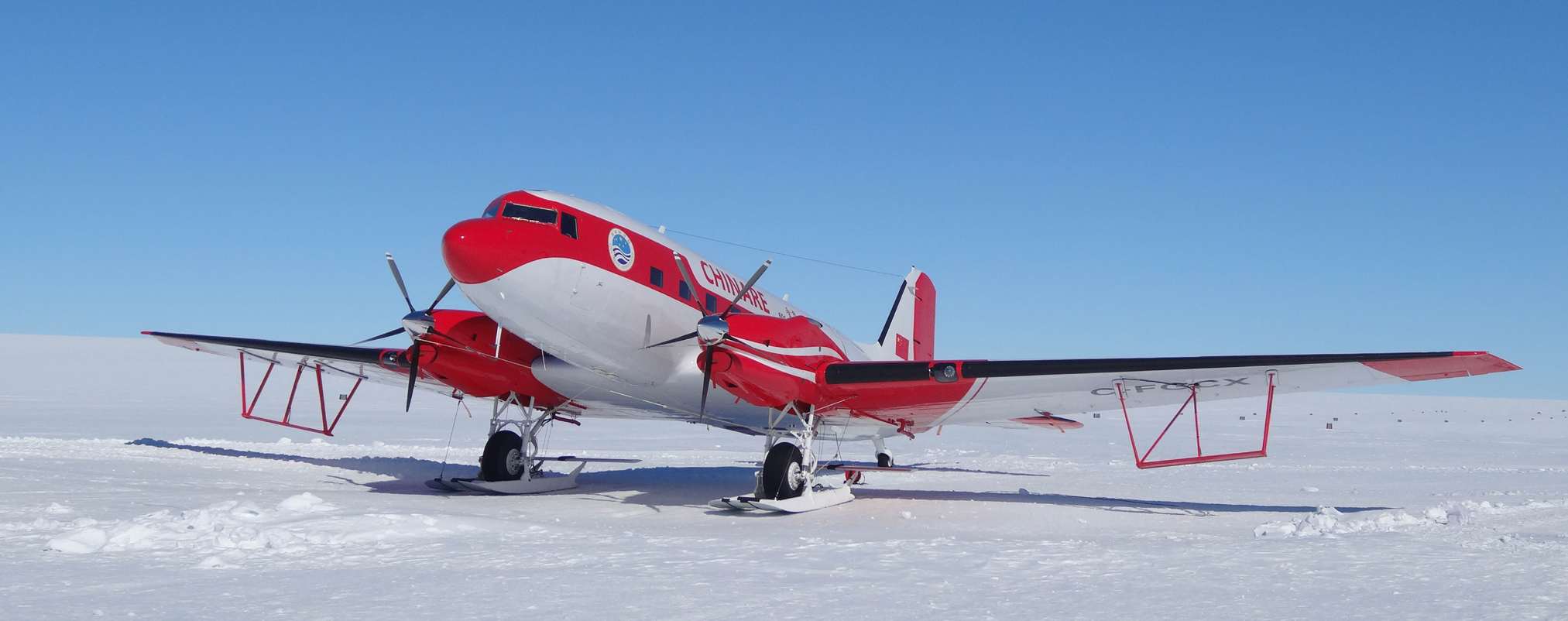
Fig. 1. The Snow Eagle 601 fixed wing ski-equipped aircraft comprising the Chinese polar airborne geophysical platform equipped with RES (the Snow Eagle IPR), gravity, magnetometer, GPS and other instruments.
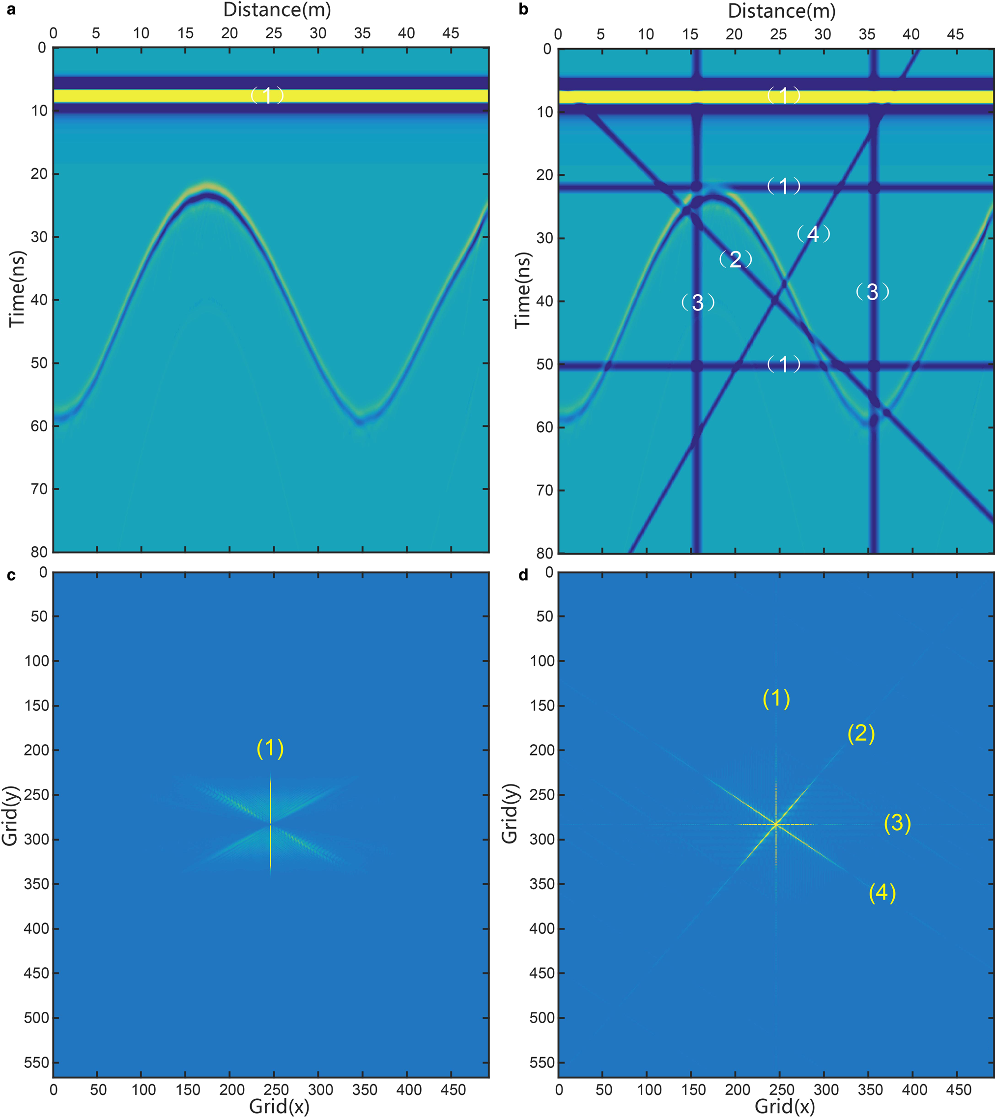
Fig. 2. Numeric RES record with appended strips and their respective 2-D FFT spectra. (a) Original numeric record. (b) Record in (a) but with added horizontal, vertical and inclined strips. The blue bar (2) is a strip with a dip angle of 45°. The blue bar (4) is a strip with a dip angle of 120°. (c) 2-D FFT frequency spectrum of the record in (a). The vertical yellow line (1) is the frequency spectrum of the horizontal air wave, corresponding to yellow bar (1) in (a). (d) 2-D FFT frequency spectrum difference of (a) and (b), which removes the synthetic RES record and leaves only the pure strip spectrum. The yellow line numbers (1), (2), (3) and (4) correspond to the horizontal, vertical and inclined strips with different dip angles.
Discrete wavelet decomposition
The wavelet transform is a popular tool for signal analysis and image processing. It has been widely used in filtering, de-noising, signal enhancement, border detecting and indexing (Mallat, Reference Mallat1989, Reference Mallat1999; Daubechies, Reference Daubechies1992). For a discrete function f(k), it can be decomposed approximately into the sum of the products from a set of basic functions ψ n(k) and corresponding coefficients a n:
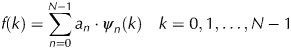 $$f\!(k) = \sum\limits_{n = 0}^{N-1} {a{}_n\cdot \psi _n(k)} \quad k = 0,1, \ldots, N-1$$
where a n are the undetermined coefficients and ψ n(k) are orthogonal wavelets. The scalar product of every two wavelets ψ n(k) meets the criterion:
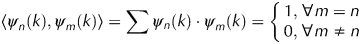 $$\langle \psi _n(k),\psi _m(k)\rangle = \sum {\psi {}_n(k)\cdot \psi _m(k)} = \left\{ {\matrix{ {1,\forall m = n} \cr {0,\forall m\ne n} \cr}} \right.$$
The coefficients a n can be calculated by simple scalar products of the function f(k) and wavelets ψ n(k):
 $$a_n = \langle f\,(k),\psi _n(k)\rangle $$
To improve calculation efficiency, discrete wavelet transforms use dyadic splitting (Burrus and others, Reference Burrus, Gopinath and Guo1997; Münch and others, Reference Münch, Trtik, Marone and Stampanoni2009), and decompose the input signal into a low frequency by applying a low-pass and a high-pass filter, respectively. The dyadic decomposition is repeated until it reaches the desired level, L. The decomposition results yield a set of coefficients, including a low-pass band and coefficients corresponding to wavelet functions at different scales.
For 2D signals f(x, y), decomposition is undertaken to form four sets of coefficients C l, C h, C v and C d, where C h, C v, C d are the horizontal, vertical and diagonal details bands, respectively, and C l is the low-pass band. C l can be decomposed continuously until it reaches L. The number of coefficients in each of the bands is 1/4 of the number in the original band. Thereby, 2-D multi-scale wavelet decomposition of level L yields the relationships:
 $$\eqalign{f\,(x,y) & = \sum\limits_m {\sum\limits_n {{\rm C}{}_{{\rm l}L,m,n}\cdot \varphi _{L,m,n}(x,y)}} \cr & + \sum\limits_{l = 1}^L {\sum\limits_m {\sum\limits_n {C_{hl,m,n}\cdot \psi _{hl,m,{\rm n}}(x,y)}}} \cr & + \sum\limits_{l = 1}^L {\sum\limits_m {\sum\limits_n {C_{vl{\rm,} m,n}\cdot \psi _{vl,m,n}(x,y)}}} \cr & + \sum\limits_{l = 1}^L {\sum\limits_m {\sum\limits_n {C_{dl{\rm,} m,n}\cdot \psi _{dl,m,n}(x,y)}}}}$$
Here, φL,m,n(x, y) is scaling function and ψ hl,m,n(x, y), ψ vl,m,n(x, y), ψ dl,m,n(x, y) are 2-D wavelet functions. Consequently, the 2-D signal f(x, y) can be expressed with a set of coefficients in wavelet domain, W, as follows:
 $$f\,(x,y)\Leftrightarrow w = \{ c_{lL,m,n},c_{hl,m,n},c_{vl,m,n},c_{dl,m,n}\} $$
Conversely, the original signal can be recovered by an inverse wavelet transform. In the wavelet domain, processing can be undertaken on discrete components to realize signal de-noising.
2-D frequency spectrum and wavelet features of strip noise
2-D Fourier spectrum of strip noise
A synthetic record made by GPRMAX is shown in Figure 2a for 2-D DFT analysis. Horizontal, vertical and diagonal strips were artificially added to the record (Fig. 2b). A 2-D DFT image of the original record, and the striped records, were then analyzed and compared (Figs 2c and d). While the horizontal first-break air wave, shown in Figure 2a, leads to a vertical linear spectrum (Fig. 2c), reflectors usually spread into the Fourier domain since they present different slopes, as opposed to strip noise which has a constant slope in the recorded data. The 2-D DFT spectrum of pure strip noise, in Figure 2d, demonstrates obvious linear features. So, the first break in the RES record can be considered as a horizontal strip noise, and therefore can be targeted for removal.
Wavelet features of strips
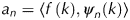
To understand the wavelet features of the strip noise, wavelet composition was performed on the synthetic record that had horizontal, vertical or inclined strips added (see R1, R2 and R3 in Column C1 in Fig. 3). Four levels of wavelet decomposition were undertaken on the striped records to obtain the components C h, C v, C d and the low-frequency approximation component, C l, which will be composited into components C h, C v and C d (see column C2 in Fig 3) in next level. The reflection wave and strips appear in components C h, C v or C d. The reflection wave appears in all components. However, horizontal strip noise only exists in C h. Similarly, vertical strips only exist in C v. Inclined strip noise appears in all components, however.
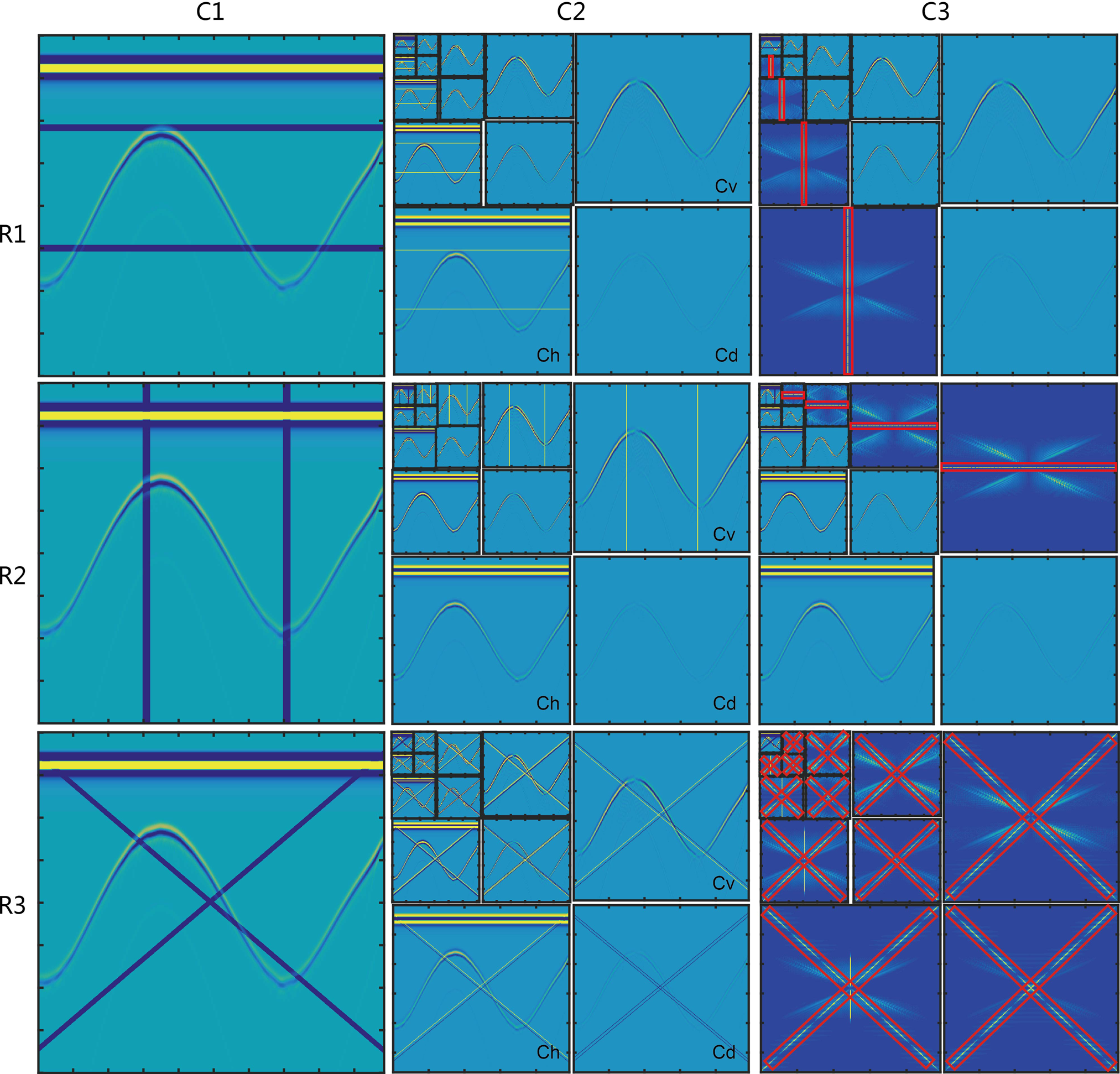
Fig. 3. Wavelet components and 2-D Fourier spectra of synthetic RES records with strip noise. R1, R2 and R3 display wavelet analysis to horizontal, vertical and inclined strips, respectively. Column C1 represents images of RES records with appended strips, which derive from the synthetic records in Figure 3a. Column C2 shows four levels of wavelet decomposition. Column C3 provides the 2-D Fourier spectrum of part components that keep the strip noise information. The horizontal strip noise only appears in the C h components. So, we just analyze the Fourier spectrum within the red box in R1C3. Similarly, the vertical strip noise only appears in C v components. So, we just analyze Fourier spectrum of C v components, and label the line spectrum of the strip noise within red box in R2C3. Inclined strip noise exists in all components C h, C v and C d. So, we analyze Fourier spectrum of all three components and label the line spectrum of strip noise within the red box in R3C3.
2-D Fourier analysis on the components containing strip noise information is listed in Column C3 of Figure 3. For horizontal and vertical strip noise, we simply need to perform a spectral analysis on the C h or C v component. But, for inclined strip noise, all components need to be processed spectrally. The Fourier analysis of wavelet components revealed that the spectrum of strip noise from wavelet components replicates the same linear feature. Because of this, we can eliminate the linear spectrum in necessary components of each wavelet level and then restore the de-striped record by an inverse wavelet transform.
Strip noise removal technique based on wavelet decomposition and 2-D DFT filter
The simplest way to remove horizontal or vertical strip noise is by deleting the component C h or C v, and then performing an inverse wavelet transform. A disadvantage of this approach is that the component C h or C v also includes spectra from the signal. Hence, by using direct deletion the desired signal will likely be affected as a consequence of the operation. Additionally, the technique is unsuitable for inclined strip noise removal, because the inclined strip message exists in all components (Fig. 3 R3). In short, direct deleting of strip noise is not an optimal solution.
While the 2-D Fourier spectrum of strip noise, and its wavelet components, has a constant slope (as shown in Figs 2 and 3), that from the reflection wave has a wider spectrum distribution (as illustrated by the pinnate distribution in Fig. 2c). As a consequence, damping or masking the narrow linear spectrum (red box marked as C3 in Fig. 3) will make a minimal impact on the desired reflection wave. Some filtering methods have been proposed for de-striping (Chen and others, Reference Chen, Lin, Shao and Yang2006; Liu and Morgan, Reference Liu and Morgan2006; Zhang and others, Reference Zhang, Shi, Guo and Huang2006; Wang and Fu, Reference Wang and Fu2007), but most of them use surgical damping, or masking in the frequency domain, based on the frequency spectrum difference between the strip noise and the reflection wave.
Here, we use a simple band-notch filtering method perpendicular to the strip noise to damp its linear spectrum in the wavelet domain (Münch and others, Reference Münch, Trtik, Marone and Stampanoni2009). Its function can be expressed as:
 $$g(x,y) = 1-e^{-(y^2/2\cdot \sigma ^2)}$$
where x is the direction of linear spectrum of strip, and y is the perpendicular direction to x. In programming, x and y need to be projected to the real coordinates. σ determines the width of filtering along y, which can be adjusted according to filtering need. Since the 2-D DFT spectrum of strip noise has a linear feature in both real data and its wavelet components, notch filtering can be implemented to the 2-D spectrum of wavelet component, which contains linear strip spectrum, allowing its removal. Then, the removed spectrum can replace the original spectrum and a reconstructed wavelet component can be completed by inverse Fourier transform.
The steps of strip noise removal can be summarized as follows: (1) wavelet decomposition on the radio-wave signal; (2) 2-D DFT Fourier analysis on specific components containing strip noise spectra; (3) damping the linear spectra of these components by using formula (6); then (4) inverse DFT and inverse wavelet transformation to form the de-striped record. For each of the three strip types the details of the procedure are different, requiring damping of the object to adapt to the type of strip noise being processed out (Fig. 4). Gaussian damping only eliminates long-narrow linear areas in the 2-D DFT spectrum, retaining the signal information outside of the area being scrutinized for processing (Fig. 5).
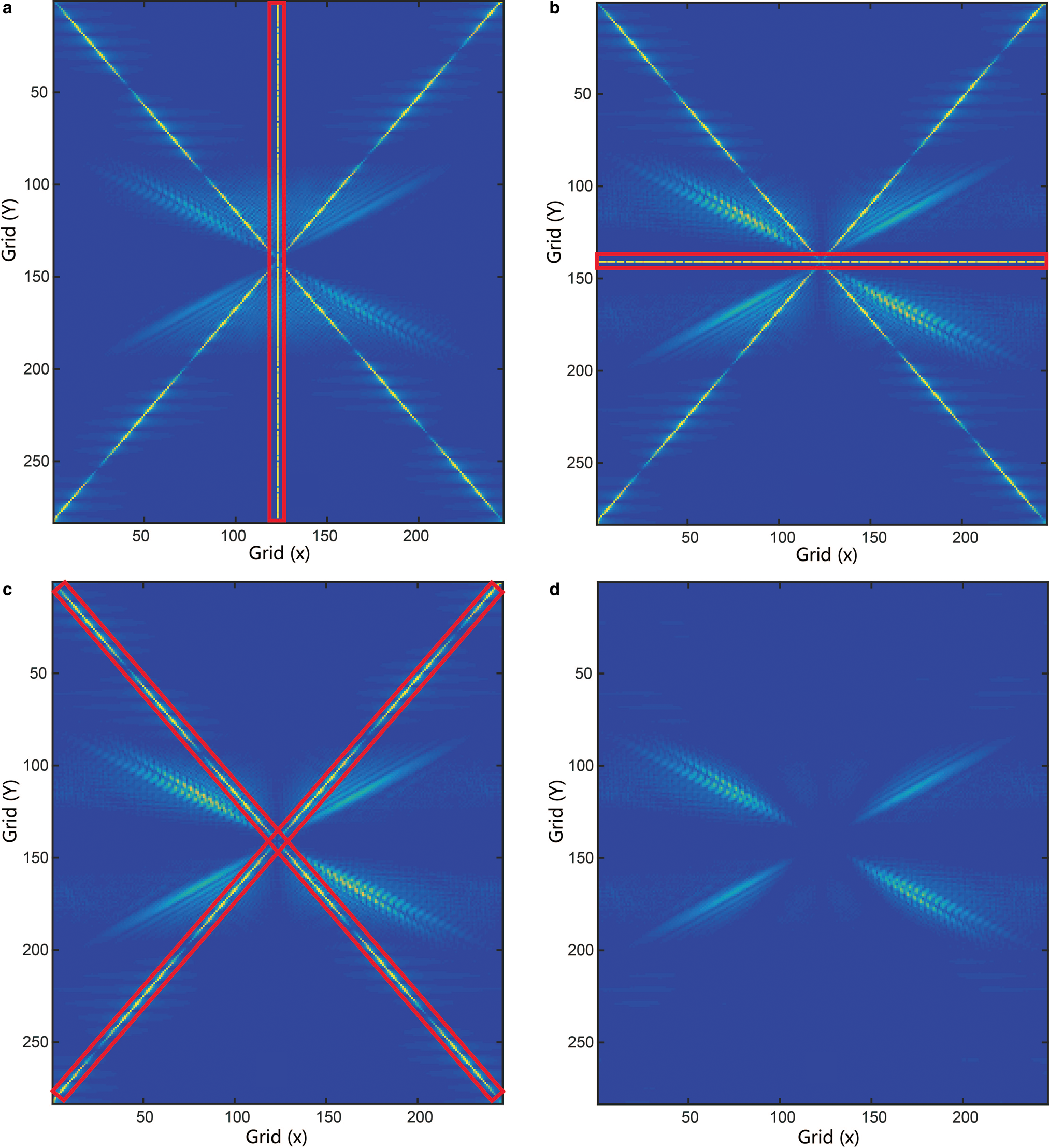
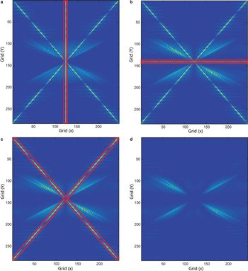
Fig. 4. Comparison of 2-D frequency spectra of wavelets among different strips. (a) Horizontal, (b) vertical and (c) inclined strip noise, marked with red boxes. (a) and (b) Correspond to the spectra of C h and C v, respectively. (c) Is the result of damping the linear spectrum of horizontal strip noise using Eqn (6) to leave the inclined strip spectrum. (d) Result of removing inclined strip noise shown in (c).
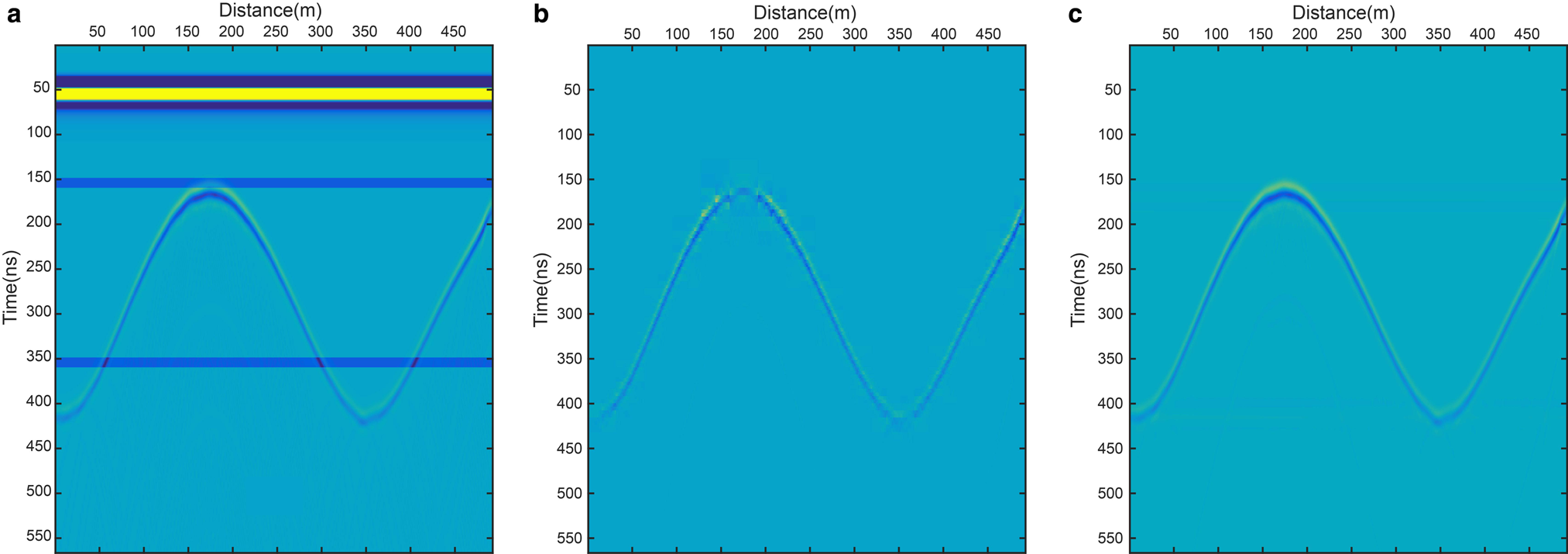
Fig. 5. Comparison of direct deleting of components and damping strip methods. (a) Synthetic record with horizontal strip noise. (b) Artifact left after deleting component C h. (c) Artifact left after using the damping Eqn 6 on the component C h.
RESULTS
Testing using hypothetical numerical modeling
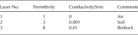
We set a 2-D model to replicate a (non-glaciological) GPR transect 30 m in length, 5 m deep. It has three layers as follows: the top layer is the free air; the middle layer is soil; and the bottom is rock. The depth of interface between the soil and rock varies from 1.5 to 4.6 m along the profile (Fig. 6a). The electrical parameters used are listed in Table. 1.
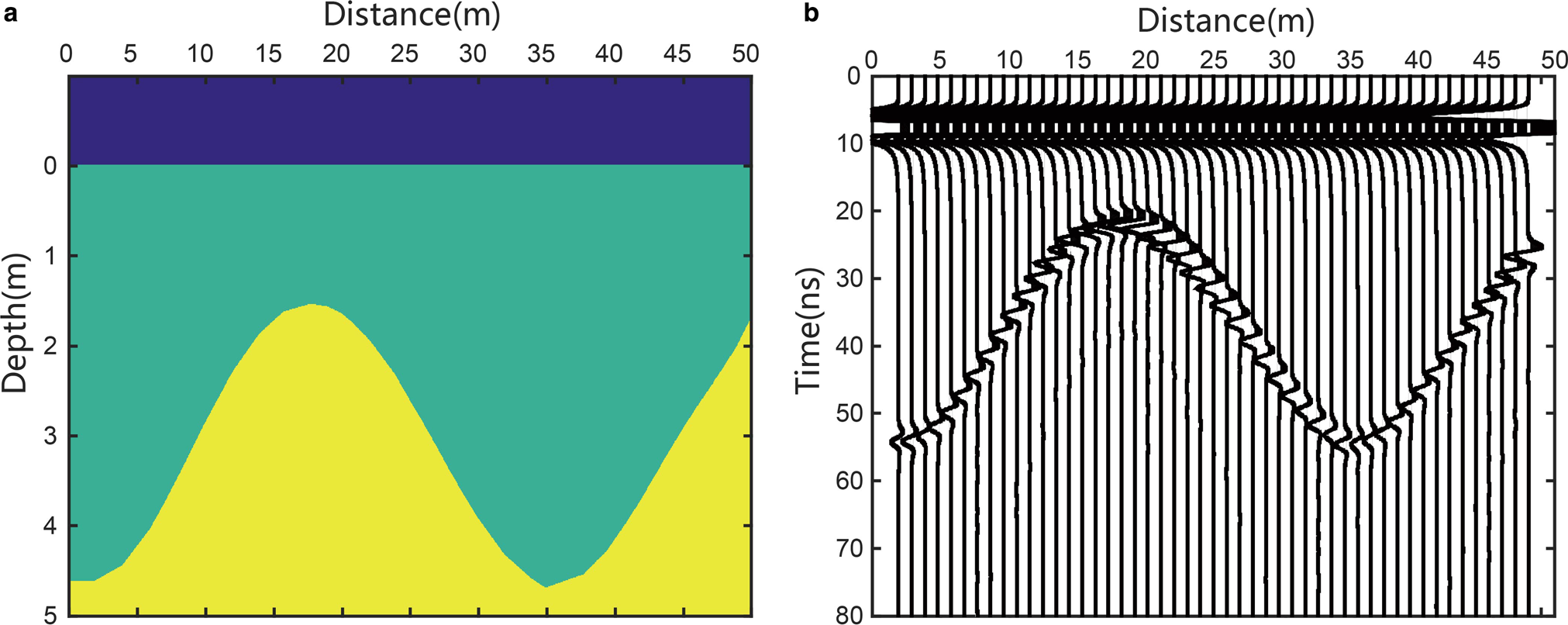
Fig. 6. The forward model boundary conditions and its synthetic RES record. (a) Forward model with parameters listed in Table 1. (b) Synthetic record generated by GPRMAX. The real interval between traces is 0.1 m. To display the waveform clearly, one trace is selected out from per 10 traces.
Table 1. Model parameters
A 200 MHz radar record was generated with GPRMAX according to the constructed geological conditions in Figure 7a. We then added two horizontal strips at times 150 and 350 ns, two vertical strips at distances of 150 and 350 m, and two inclined strips with dip angles of 45° and 135°, as shown in Figure 7b.
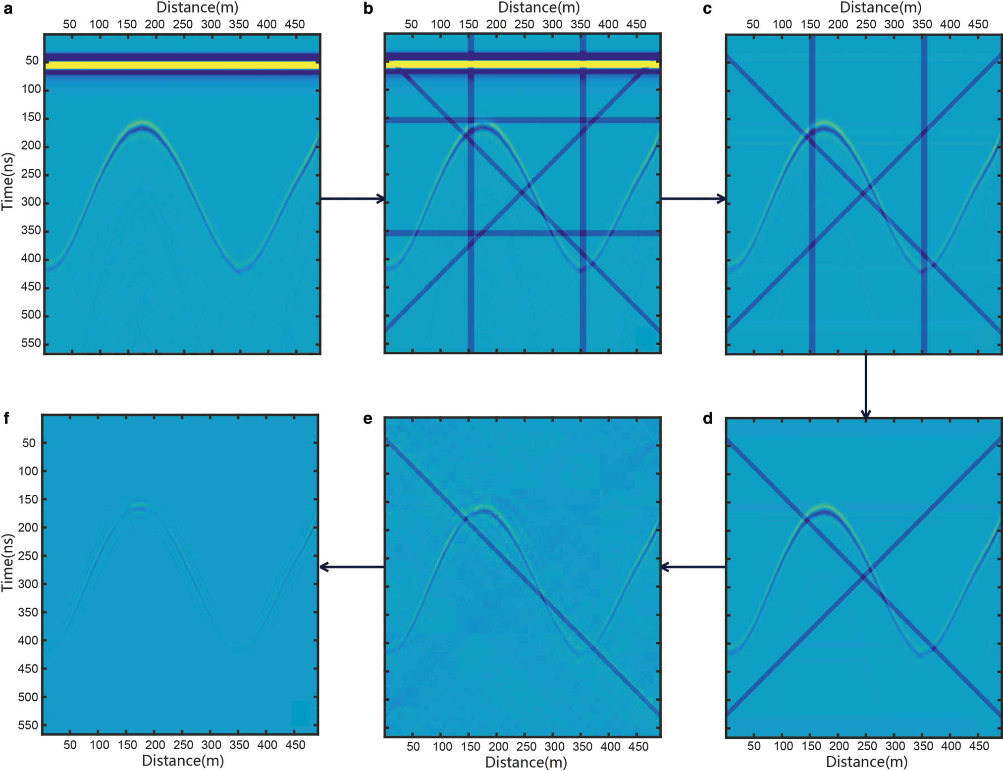
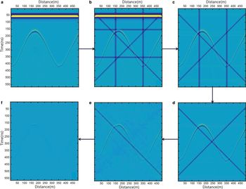
Fig. 7. Strip noise removal, step by step using combined wavelet and 2-D FFT filtering method. (a) Original synthetic RES record with 500 traces and 500 samples. (b) Record appended with horizontal, vertical and inclined strip noise. The black arrow points to the sequential order of the de-striping process. (c) Result of removing horizontal strip noise, including the first break air wave. (d) Result of removing vertical strips. (e) Result of removing inclined strip noise with a dip angle of 135°. (f) Result of removing the inclined strip noise with dip angle of 45°.
Using the method of combined wavelet and 2-D DFT filtering, we removed the strips (Fig. 7). Figure 7c shows the removal of either the horizontal strip or the air wave. In general, this method leads to the thorough removal of horizontal and vertical strips, and keeps the effective reflection well. However, the effective reflection has some loss of information after the inclined strips are removed.
Airborne RES example
Obvious horizontal strip noise is present within the RES records collected by the Snow Eagle IPR (Fig. 8a). Besides signal enhancement and other routine processing techniques, we employed the method described above to remove the strip noise.
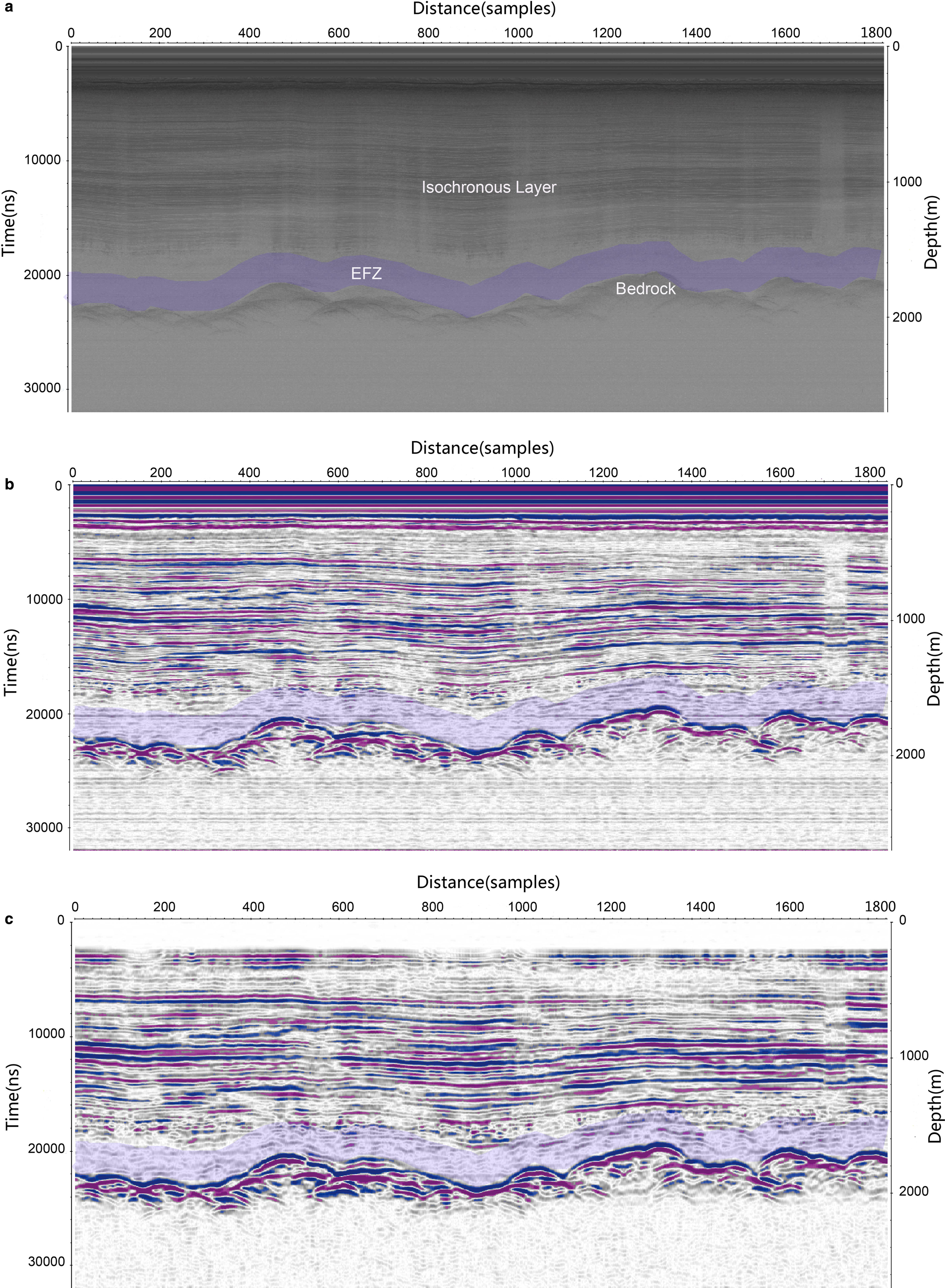
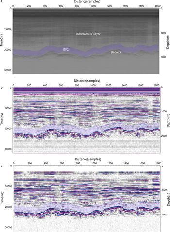
Fig. 8. Comparison of Snow Eagle IPR raw data, signal-enhanced data and strip-removed data. (a) Raw RES data. The transparent blue belt labels the EFZ zone. (b) RES record after signal enhancement and other routine processing. (c) Record after horizontal strip removing.
The EFZ zone is the deepest part of the ice sheet, close to the ice-sheet bed, usually several hundred meters in thickness (Fig. 8). A major feature of the EFZ is that the echo vanishes sharply, leaving an information-free belt alone the profile, beneath which a reflection from the bed normally occurs. There are several hypotheses about the physical nature of the EFZ: (1) it is related to the geothermal gradient near bed; (2) ice flow around complex topography; (3) englacial rheological variations; and (4) various combinations of these options (see Fujita, and others, Reference Fujita1999). In some cases the EFZ contains some very faint reflections and, when this happens, it may be possible to enhance the signal in order to provide important and hitherto unidentifiable information from the basal regions of the ice sheet (Wang, and others, Reference Wang, Tian, Cui and Zhang2008).
Isochronous layers and bed reflectors can be identified clearly in Figure 8a. Despite the excellent penetration of radio-wave power to the bed, there is little information from the EFZ in the RES data (Fig. 8a). After signal enhancing and DC shift processing, the isochronous layers and the bed become clearer (Fig. 8b) and some information emerges from the EFZ. However, horizontal strips also adversely affect interpretation of the EFZ. After thorough horizontal strip noise removal, the faint reflections otherwise hiding in the EFZ become more apparent (Fig. 8c). In addition, the de-striping process reveals a newly-identifiable but non-continuous layer above the EFZ (possibly due to basal accretion of ice, or sediment entrainment). Hence, by using the de-striping technique, it is possible to resolve information from the EFZ where previously no information was thought available. The possibility exists, therefore, to undertake the data processing proposed here to previously collected data where the EFZ is a prominent and potentially interesting region of the ice sheet.
Ground RES example from Dome A
CHINARE accomplished 1300 km worth of geophysical surface traverse data acquisition, between Zhongshan Station and Dome A in 2004/05. The instrument used was a dual-frequency polarized radar, pulled by snow vehicles (Fujita, and others, Reference Fujita1999). As the vehicles needed to keep contact with each other when traverse moved forward, wireless communication across the system led to vertical strip noise on the RES records (Fig. 9). Some filtering methods had previously been applied to the data, but without success in removing the noise. A subglacial valley is observed trending along the northeast-southwest direction across Dome A area, beneath more than 3000 m of ice (Sun and others, Reference Sun2009), which some consider to be an optimal site for extracting very old (~1 Ma) ice. Using our de-striping method, we were able to extract more distinct isochronous layers, aside from removing the vertical strips, so adding value to the data previously collected (Fig. 9).
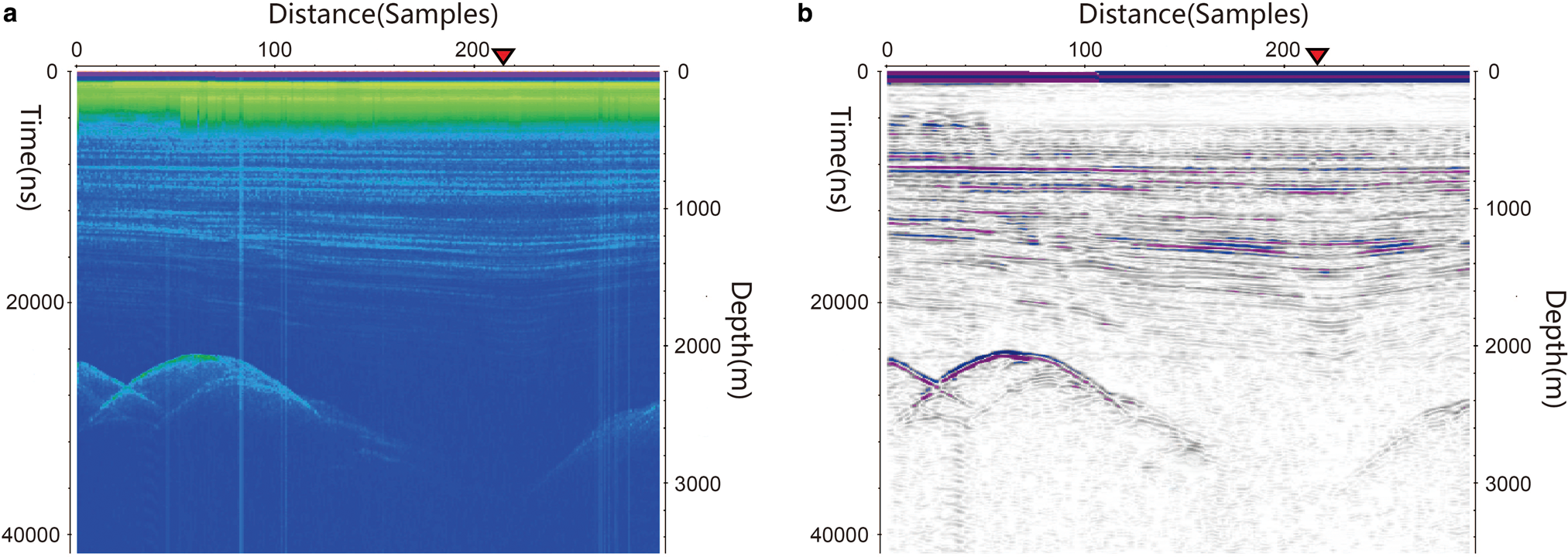
Fig. 9. Comparison before and after strip noise removal between the original RES record (a) suffering communication noise, and the processed data (b). The red triangle denotes the position of Kunlun Station at the summit of Dome A in East Antarctica, and location of the deep ice-core site.
DISCUSSION AND SUMMARY
Our de-strip method, employing mature wavelet and 2-D DFT filters, is a stable and reliable technique. But, parameter choices still have an effect on filtering, mainly concerning the wavelet transformation and 2-D DFT analysis. Here, we discuss the types of wavelet, decomposition levels and damping coefficients of Gaussian filtering.
Type choice of wavelet
We tested the effect of different wavelet types. Higher level wavelets are easier to de-strip than lower level wavelets. For example, in the Daubechies wavelet, DB45 is easier to deal with than DB 10, DB 2 and DB 1. In addition, we find that Biorthogonal wavelets are more sensitive to inclined strips. So, the type of wavelet needs to be understood prior to processing. HAAR (DB1) is the most popular wavelet, and can implement the basic requirements of strip removal, hence all the results in this paper are based on wavelet DB1.
Decomposition level
From Eqn (4) we know that, after multi-level decomposition, the last low-frequency component C l remains and retains strip messages. Strip-spectrum damping is undertaken on components C h, C v and C d, but not the last component C l. The more decomposition levels there are, the lower the proportion of strip noise remains in the final component, C l. While the decomposition level influences the quality of the strip removal, ultimately decomposition is controlled by the size of radar record, total traces and samples in time. We can only set the decomposition level less than or equal to the maximum decomposition level, which may restrict the efficiency of the technique in some cases.
Damping coefficient σ
From formula 6 we know that the damping coefficient σ determines the width of filtering. The larger the width the more of the spectrum of the effective signal will be removed, which may reduce the resolution ratio of the desired signal. So, we need to keep a balance between strip removing and the desired signal preservation. Normally, a damping coefficient σ is within the range 10.0–0.001.
Summary
We present a strip removing method, with combined wavelet transformation and 2-D DFT filtering, for use in cleaning RES data. Verified with synthetic models, and RES data from the Antarctic ice sheet, this method removes both horizontal and vertical strips well. In addition, the strong ‘first break’ in the RES record is also removed, so improving the general quality of RES data. Our method also enhances any weak signals in the EFZ, drawing out hitherto hidden information from the basal regions of the ice sheet. This method has no special limitations or requirements and so can be applied retrospectively to data collected already, potentially leading to significant new information from the basal regions of both Antarctica and Greenland.
ACKNOWLEDGEMENTS
This work is supported by the National Natural Science Foundation of China under grants 41676181, 41776186, the National Basic Research Program of China (973Program) under grant 2012CB957702, the Major Program of the National Social Science Fund under grants 13&ZD192, and the Fundamental Research Funds for the Central Universities 2018QNA3013. MJS is supported by NERC Grants NE/H021078/1, NE/M000869/1 and NE/K004956/2, and a Global Innovation Initiative (GII) award from the British Council. JSG was supported by the GII award, National Science Foundation grant PLR-1543452, and the G. Unger Vetlesen Foundation. We thank all members of the CHINARE 32nd expedition for the data collected on this program. This is UTIG contribution #3144. We thank Ettore Biondi and four anonymous referees for providing constructive reviews of our work, which improved the paper considerably.


 Open access