


Introduction
A dominant feature of sea-ice deformation in both the Antarctic and Arct ic regions is the presence of substantial high-frequency variability, typically with considerable power at inertial frequencies. These high-frequency motions can contribute substantially to the mass budget of the ice (Heil and others, 1998) and in some cases modify the air-sea heat exchange by up to 50 %.
This high-frequency content of the motion is in contrast to the wind forcing which occurs at much lower frequencies. Moreover, the oscillatory character of the motion has been related to ice concentrations and interaction using field observations (Hibler and others, 1974). These observations typically show a substantial “quelling” of the inertial oscillations under compact high-ice-interaction conditions. Since at high latitudes the inertial period is close to tidal periods, this deformation in tidally active areas can be amplified by the inertial resonance, a result which is suggested by observations of pack-ice deformation in the western Weddel! Sea (Geiger and others, 1998).
In almost all sea-ice dynamics models both with and without ice interaction, inertial motion is typically over-damped due to the method of coupling the ice with the oceanic boundary layer. This is because the drag formulation used in ice models assumes an averaging over time-scales that are long compared to the inertial period. This averaging procedure effectively decouples the ice mass from the mass of the dynamically active ocean boundary layer which also undergoes inertial oscillations (see, e.g., Reference MePheeMePhee, 1978).
The higher-frequency motion can be formulated more consistently by including higher-frequency motions in the boundary layer. This can be done by using a vertically integrated boundary-layer model (MePhee, 1978) which essentially locks the ice to the oceanic boundary layer in a manner such that the long-term average behavior is the same as in current numerical models. This type of slab boundary-layer model has been very successful (MePhee. 1978) in predicting inertial motion under ice-interaction-free conditions. This procedure has not, however, been carried out in conjunction with a fully interactive sea-ice model. While this “imbedding” procedure will induce higher-frequency motion in the ice drift, whether or not higher-frequency deformation (differential drift) might be pro duccd is less clear. The hypothesis here is that within a fully interactive ice model, coupling effects could well produce a substantial deformation signal. However, this process has not been examined to dale.
In order to develop a more consistent treatment of ice drift under fluctuating wind fields, we develop and numerically investigate here a vertically integrated ice/ocean boundary-layer system in the context of an interacting ice field. Since the focus here is on the physical processes, a linearized boundary-layer formulation is used together with an idealized 1.5-dimensional dynamic—thermodynamic sea-ice model. The configuration of this model is examined with in the context of a winter deformation experiment in the East Antarctic sea-ice zone (Reference Worby, Bindoff, Lytle, Allison and MassomWorby and others, 1996). During this time, a number of drifting buoys were monitored hourly for studies of sea-ice drift and deformation (Heil and others, 1998). Detailed atmospheric forcing data are also available for model comparison.
Imbedded Model Formulation
Boundary-layer drag in general can be formulated in terms of a high-turbulence layer of water very close to the ice which then matches to an “Ekman” layer region at further depth where the vertical eddy viscosity can be considered basically constant Within this context, turning angles between the ice-drift direction and the stress of the ocean and the ice depend on the variation of the turbulence close to the ice. Dependence of the drag on the ice velocity, on the other hand, depends on the scaling of the turbulence with the ice velocity. Within this context a critical point is that there is effectively no (or very low) stress at the bottom of the boundary layer (Ekman layer portion). Consequently the ice-ocean boundary layer can be thought of as free to move, and under a pulse will undergo inertial oscillations with very little damping. Essentially it is as if the ice—ocean system were on a “frictionlcss” table. Hence, while internal stresses within this boundary layer can affect the details of turning angles and turbulence change with depth, they cannot modify the overall momentum balance of the aggregate boundary layer. Indeed, this overall momentum balance leads to the classic argument that the divergence of the Ekman transport is proportional to the curl of the wind stress independent of the turbulence characteristics of the oceanic boundary layer.
Governing Equations
An approximation often used for inertial studies is to consider the ice-ocean system to move as a slab. Within this context there will be fixed turning angles between different portions of the oceanic boundary layer and the ice. While this slab approach is certainly an approximation, the physical notion here is that turbulence-induced stresses with in the boundary layer are substantial and lead to adjustment time-scales that are rapid compared to the inertial period. Consequently, over several inertial periods the motions at different portions of the boundary layer are highly coherent, and hence may effectively be viewed as locked together. We also note that formulations taking the ice stress to depend on the ice velocity implicitly assume a slab formulation with an average over several inertial periods. Such models (see, e.g., Geiger and others, in press) do well for lower-frequency ice motion but yield no significant inertial motion.
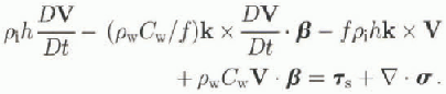
With in the slab formulation the turning angles and ice-water stress formulations may be maintained (following MePhee, 1978) by taking the mass of water transported to be related to the ice velocity. Taking the simplest case of the water drag linear with the ice velocity, Mw, the boundary-layer mass transport is given by:
where V is the ice velocity relative to the background gcos-trophic flow, pw is the water density, ƒ is the Coriolis parameter, Cw is a water-drag coefficient, and β is a rotation operator such that
where β is a turning angle and x arid y are unit vectors. The total mass transport M of the boundary-layer system consisting of ice plus water is given by
where h is the ice thickness and pi is the ice density. Since we consider that there is negligible drag on the bottom of the boundary layer, the only forces acting on the ice boundary-layer system are given by the surface wind-stress Coriolis force and ice interaction forces. Consequently, M obeys an equat ion of motion
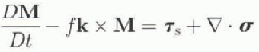
where σ is the ice stress tensor, Ts is the surface stress and D/Dt is the substantial time derivative. Expressing all the terms of the equations of motion in terms of the ice velocity, we obtain
It is clear that in a steady-state condition where all the time derivatives are zero this equation yields the conventional ice-motion equations (e.g. Hibler, 1979) with a linear drag ![]() at a turning angle β relative to the negative ice-drift direction. However with time-dependent forcing, the integrated equations allow the ice and upper ocean to contain inertial motion.
at a turning angle β relative to the negative ice-drift direction. However with time-dependent forcing, the integrated equations allow the ice and upper ocean to contain inertial motion.
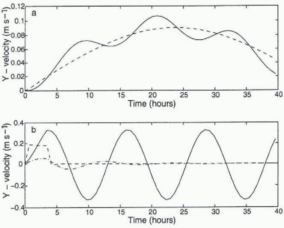
Fig. 1. Simulated velocity for 1m thick sea ice with (solid line) and without (dashed line) inertial imbedding, (a) is for ![]() with t in hours; (b) is fora step-function wind of
with t in hours; (b) is fora step-function wind of ![]() for 3.5 hours and zero thereafter. The dotted line in (b) is for extremely thick (5 m) ice (see text).
for 3.5 hours and zero thereafter. The dotted line in (b) is for extremely thick (5 m) ice (see text).
Numerical Solution Procedure and One-Dimensional Example
To carry out a numerical solution of the ice-drift equation in a Lagrangian grid described below, we make use of an explicit time-stepping procedure with all of the Coriolis terms in the above equation centered in time. Forward Euler time-stepping is used for the time derivatives, and the ice interaction and wind-stress terms are treated explicitly. This necessitates small time-steps of the order of 1 s tor the viscous plastic rheology. This solution procedure insures that the inertial terms are centered in time and that there is no spurious damping of the inertial motion. For these simulations and the interacting ice-field simulations discussed later in the paper we take the numerical values of the variables in Equation (5) to be: 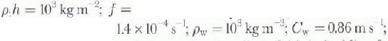 and β = 30°.
We examine the effect of this imbedding for free ice drift (no ice interaction) for a sinusoidal wind forcing (fig. 1a) and for a step-function wind forcing (fig. 1b). Figure 1 shows veloc ity of the ice both with and without imbedding. With imbedding, the ice will undergo inertial motion which is superimposed on the steady, sinusoidal driven motion. With a step-function wind which is set equal to zero after a few hours, the system will effectively undergo inertial oscillations which are reduced only if we apply a damping term to the formulation. in the case of extremely thick ice of 5 m (fig. 1b, dash-dotted line) with passive drag, there will be some slight highly damped oscillation which is much smaller than the oscillation of the overall boundary layer. The strength of this damping provides further justification for the slab approach, as this type of interfacial stress will be in effect between portions of the oceanic boundary layer as well as between the ice and oceanic boundary layer.
Observed Antarctic Deformation Characteristics
Data taken as part of the Australian East Antarctic field experiment “HiHo HiHo” (Worby, 1996) have provided an excellent example of higher-frequency deformation. Moreover, this region is not tidally active, and consequently is felt to have primarily incrtially induced higher-frequency motion rather than tidally forced motion. Analysis of the thermodynamic consequences (Heil and others, 1998) of ice deformation from this field experiment has shown that this higher-frequency motion can in some cases more than double the area-averaged ice-formation rate.
The basic characteristics of the drift and deformation record taken during this experiment show a strong defor-mation signal largely dominated by deformation perpendicular to the coast, together with drift variations that are larger parallel to the coast. This drift is also found to be well correlated with wind motion for motion along the coast, but somewhat less so for motion perpendicular to the coast. Ίο quantify this character, we calculate a linear least-squares fit of the drift velocity to surface wind velocity, forcing the ice velocity to zero at zero wind speed.
The best-fit equation is given by
where u + iv and uw + ivw are complex ice and wind velocities in an arbitrary coordinate system. This result corresponds to the ice having a drift relative to the buoy wind of about 1/40 of the wind speed in a direction about 10° to the left of the wind direction.
Representing the ice velocity in a coordinate system aligned with the coast, the predicted and observed velocities are shown in Figure 2. As can be seen, the local wind at the buoy predicts the alongshore ice motion very well, but does less well for the ice motion perpendicular to the coast which displays less variance in general.
While the alongshore motion is substantial, much of the deformation occurs perpendicular to the coast, which is illustrated in Figure 3 where we show the components of the strain-rate tensor parallel and perpendicular to the coast. The results show a stronger oscillation in the deformation early on in the record, even though the wind is relatively smooth over this time interval. Frequency analysis of this data reveals much of the power of these oscillations is at the inertial period (Heil and others, 1998).

Fig. 2. Observed and simulated velocity components (u and ν) in a coordinate system which is aligned to the coastline (see Fig. 4). Also shown are the x and y components of the wind (dotted line).
Numerical Investigation of Inertial Oscillations in An Interacting Ice Field
Based on the buoy-deformation characteristics outlined above, a 1.5-dimensional dynamic—thermodynamic model with a 40 km resolution was constructed as shown in Figure 4. in this model, full two-dimensional ice dynamics is assumed, but all variations along the coast are assumed to be zero. This formulation allows shear strength as well as compressive stress to be utilized in the formulation, while still allowing a clearer analysis of the essential characteristics of the inertial imbedding tobe examined. ALagrangian grid formulation is utilized together with a dynamical formulations for the ice interaction, as used by l.eppäranta and Hibler (1985) for ice-margin analysis. For thickness-strength coupling, a relationship between ice strength (P), ice thickness and compactness (A),
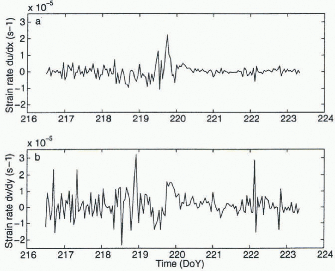
Fig. 3. Components of the strain-rate tensor (a) du/dx (parallel to coast), and (b) dv/dy (perpendicular to coast), for a buoy deployed in the sea-ice zone during the East Antarctic “HiHo HiHo” field experiment.
was assumed. Because a Lagrangian grid was used, the conservation equations for compactness and thickness simply involve multiplying the concentration and thickness by the divergence rate to obtain time rate of changes of these variables (Reference Leppäranta and HiblerLeppäranta and Hibler, 1985). Numerical values were the same as used in the one-dimensional example cited earlier, together with initial conditions of A = 0.95 and h = 1 m in all simulations. in cases without ice-thickness and ice-compactness evolution equations included,^ and h will be constant.
Two types of simulations were carried out, both with and without inertial imbedding. in the first ease, only the momentum equations were utilized without any thickness-strength coupling, whereas in the second case the compactness and thickness were allowed to evolve according to conservation equations (Hibler, 1979). Two types of forcing were used: a half sine wave of wind, and a constant wind which was dropped to zero after about 4 hours.
The salient results from these simulations are shown in

Fig. 4. Coordinates for the 1.5-dimensional model domain. The wind stress is applied in a spatially constant manner along the y axis in all numerical experiments.
Figures 5-9. in the absence of ice-lhickness-strength coupling with a sine-wave forcing (Fig. 5) there is an oscillation at all gridcells. The inertial motion is seen, and is similar at varying distances from the coast. This oscillation is not present without imbedding. Consistent with plastic flow characteristics (e.g. Leppäranta and Hibler, 1985) the ice moves rigidly with failure at the coast. Because ofthis rigid motion there is essentially no deformation at the inertial period, except right at the coast.
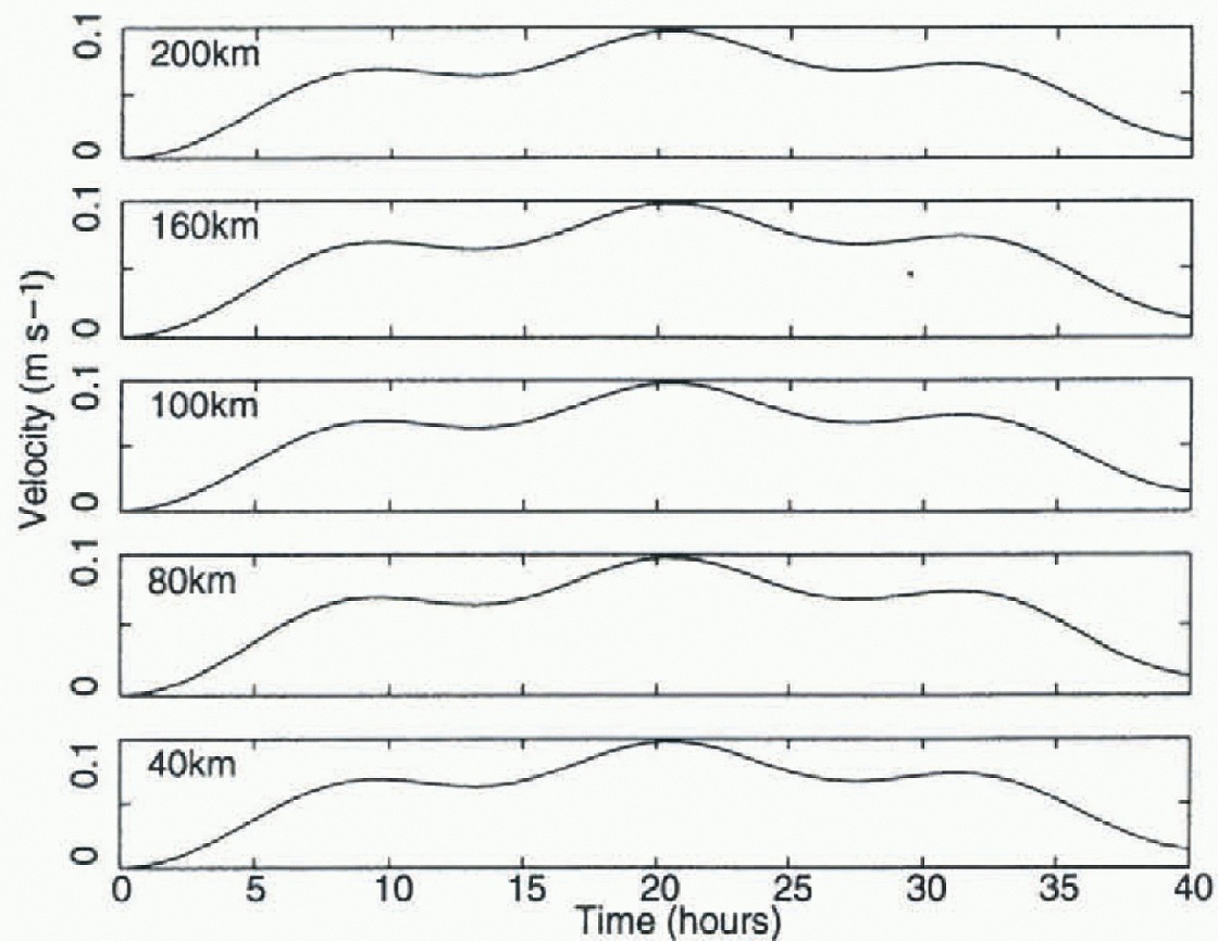
Fig. 5. Time series of sea-ice velocity perpendicular to the coast at offshore gridpoints of gridcells centered 20,60,100,140 and 180 km away from the coast for the imbedded model without ice-thickness strengthening. A spatially uniform sine-wave windforcing was used as in Fig. 1. Alt velocities are essentially the same.
When thickness strength coupling is added, however, there is a substantial effect. As seen from the half-sine-wave results shown in Figure 6, we see a ridging front move outward both with and without imbedding. This is illustrated by the velocity decreasing in magnitude as the front moves outward from the coast. This is the simplest case ofa kinematic wave (Hibler and others, 1983). With imbedding added, however, there is a pronounced oscillation at the inertial period, with some phase shift as the ridging front moves outward. As the compactness changes, the phase and orientation of these inertial motions vary as a function of space. This results in significant differential motion and hence deformation.
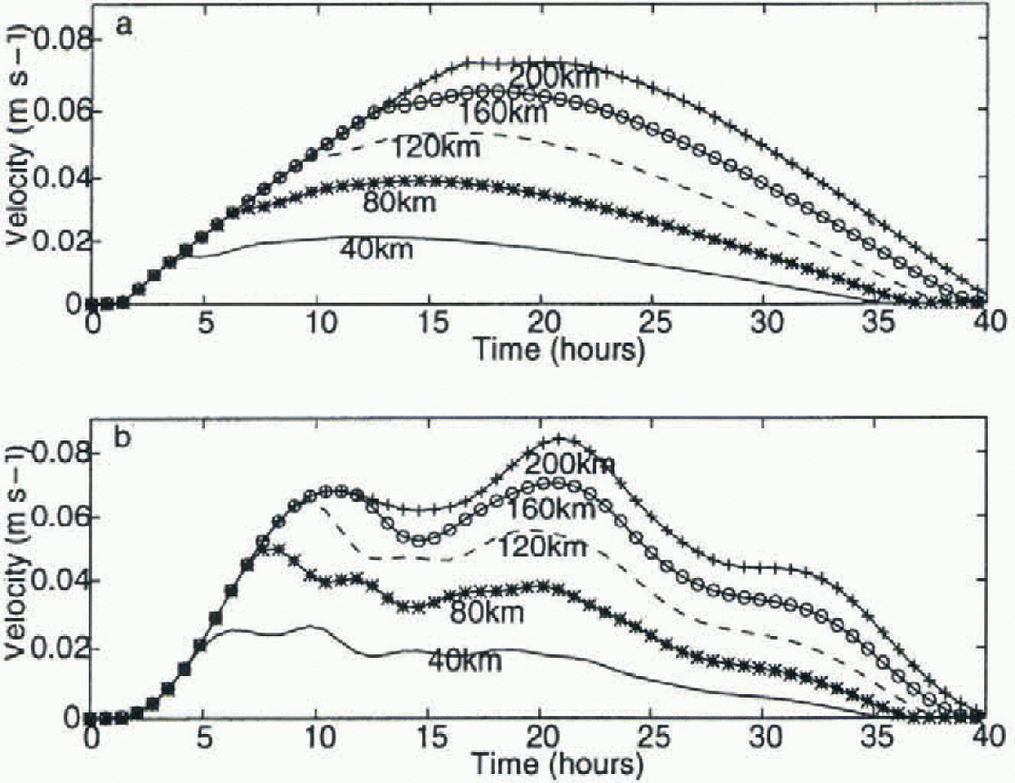
Fig. 6. Time series of modelled sea-ice velocity perpendicular to the coast for gridcells centered 20, 60, 100, 140 and 180 km away from the coast, including ice-thickness strengthening without (a) and with (b) inertial imbedding fora sine-wave wind forcing.
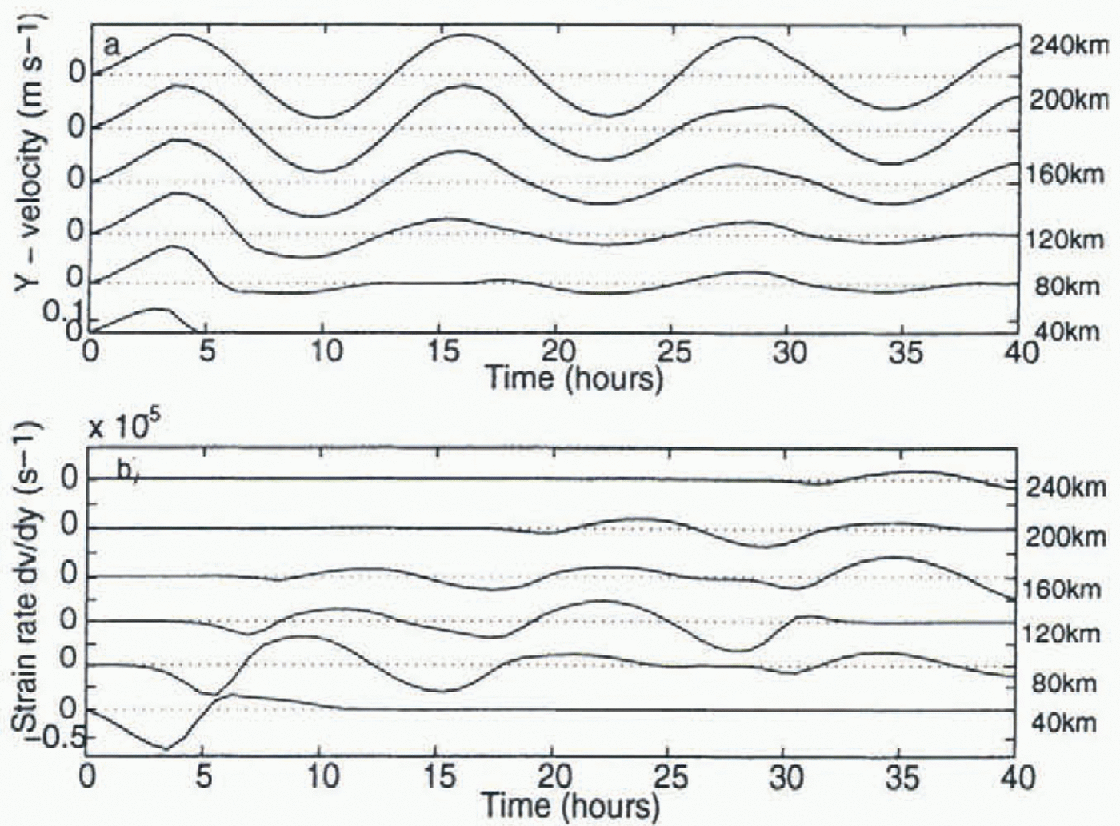
Fig. 7. Time series of (a) the sea-ice velocity and (b) the divergence rate for the imbedded model with a step function wind forcing of y = — 0.2 Ν rn which is stopped after 3.5hours. Both the velocities and the strain rate are shown offsetfor clarity.
These oscillations are notably present even in the absence of wind, as can be seen from Figure 7. Here we show results from the imbedded model where a sinusoidal wind is reduced to zero after about 4 hours. After the wind ceases, the system inertially oscillates, with some damping due to convergence in different regions caused by the ice interaction. Because there is an ice-boundary-laycr system which conceptually can be thought of as largely resting on a “frictionless surface”, this type of behavior is quite reasonable. The deformation is maximum near the coast. However, due to the phase shift of kinematic waves propagating out, there is also a strong deformation signal a substantial distance from the coast (fig. 7b). The reasonable magnitude agreement between observation and simulation of the strain tensor components for calm conditions is shown in Figure 8.
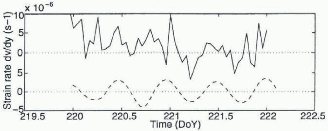
Fig. 8. Observed (solid line) and simulated (dashed line) strain-rate tensor component dv/dy perpendicular to the coast. The simulations are for a step function wind forcing some time after the wind has been set to zero, and the observations are during quiescent conditions. The two time series have been offset for clarity.
This deformation signal also leads to a substantial change in the ice concentration, with eventually a “banded” structure (Fig. 9) developing with oscillating regions of thin ice alternating spatially with ice undergoing no deformation. If there were no variations in the ice concentration along the coast (as assumed here) then bands would develop, a phenomenon often observed in the marginal ice zone. in this particular example, because of the highly non-linear nature of the sea-ice dynamics, there is only a very weak damping of these oscillations. Further analysis shows they do eventually damp out, leaving “banded” ice concentrations behind. of course, in an actual physical situation they will be damped out due to a variety of processes, including growth of sea ice in the diverging regions and lateral damping in the ocean.
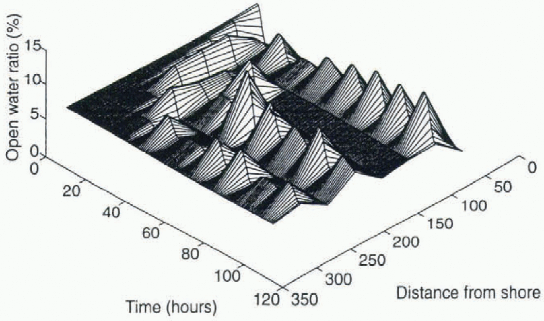
Fig. 9. Perspective view of compactness as a function of time and distance from shore, resulting from an initial pulse of wind as used in Figure 7.
The precise spacing and character of these bands will be related to the ice strength and wind force which affect the speed of the kinematic waves (see, e.g., Hibler and others, 1983). It is likely in this case that the irregular spacing is due to low spatial resolution (40 km) of the simulation. Further analysis of this phenomenon is needed to establish the essential scaling parameters. However, the main issue is that this type of phenomenon can lead to a substantial variability in the deformation, especially for a more dilute pack-ice cover as occurs in the AntarctiC. As the resolution of ice-ocean models used in climate studies increases, the importance of including this type of phenomenon becomes paramount.
Concluding Remarks and Discussion
The main thrust of this paper has been to demonstrate the effects of inertial imbedding on ice-deformation character-ist ics. The basis of this work is that although wind forcing is relatively smooth, the combination of thickness-strength coupling and inertial motion in the upper ocean conspires to create a substantial amount of higher-frequency deformation. This result is commensurate with observations, and supplies an explanation as well as a basic physical mechanism for including this physics in sea-ice dynamics models.
The results here were largely caused by the presence of a land boundary. However, in reality we would expect spatial variations in wind as well as ocean currents to be a major source of forcing to cause such variations. These characteristics would be expected to be less pronounced under very compact growth conditions such as in the ArctiC. For the looser, less consolidated Antarctic ice pack, we expect them, however, to play a substantial role in the ice mass balance.
With in the context of this investigation, these higher-frequency phenomena are basically mechanical processes controlled by stresses in the ice pack rather than body forces such as the surface wind stress. Consequently it would seem very risky to attempt to model them by statistical parame-terizations, especially since the computational efficiency of sea-ice models has recently been greatly improved (see, e.g., Reference Zhang and HiblerZhang and Hibler, 1997), allowing processes like this to be directly simulated.
While the investigations here have been mechanistic in character, they illustrate the basic character of the phenomenon and provide a justification for more detailed investigations and inclusion of inertial effects in sea-ice dynamic-thermodynamic models. Additional work regarding both more realistic boundary-layer formulations and full two-dimensional investigations is needed. Also clearly needed work is the inclusion of this type of imbedded sea-ice model together with free surface ocean-circulation models capable of including tidal forcing. Such efforts are currently under way and we hope that this work will motivate similar inclusion in coupled atmosphere-ocean climate studies.
Acknowledgements
Thanks to the numerous people who helped with the field experiment that motivated this work, including I. Allison, A. P. Worby, R. A. Massom, I. Knott, and A.V. Rada. PH. thanks the Antarctic CRC for financial support towards her visit to the Thayer School of Engineering and W.D.H. thanks the Antarctic CRC for support towards his month long research stay in Hobart. Thanks also to the anonymous reviewers whose remarks improved the final manuscript.


