1. Introduction
On 16 September 2006, on the last possible occasion in that year, Landsat 5 passed the region of the Jostedalsbreen ice cap, southern Norway, and acquired the first completely cloud-free scenes without seasonal snow outside glaciers since its launch in 1984. In the same year, many glaciers in Norway experienced their most negative mass balance ever measured (Reference Andreassen, Elvehøy and KjøllmoenAndreassen and others, 2007). These special conditions emerged after a winter with much less (–40 to –70%) accumulation than normal and three successive months (July–September) with above-average temperatures (Reference KjøllmoenKjøllmoen and others, 2007). The scenes reveal that both the margins of the ice caps and the boundaries of the numerous cirque glaciers to the north of Jostedalsbreen were snow-free (Fig. 1). We have taken this unique opportunity to create a new glacier inventory for the entire region from these two sequential Landsat Thematic Mapper (TM) scenes (path 201, row 16/17). The new inventory also contributes to the recent effort to compile a new satellite-derived glacier inventory for the whole of mainland Norway (Reference Andreassen, Paul, Kääb and HausbergAndreassen and others, 2008; Reference Paul and AndreassenPaul and Andreassen, 2009) and to complete the global glacier inventory of the GLIMS glacier database (cf. Reference RaupRaup and others, 2007).
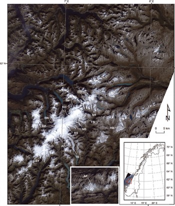
Fig. 1. Overview of the Jostedalsbreen region as seen from Landsat 5 on 16 September 2006 in a band 321 composite. The inset at the lower right shows the location of the study region in Norway; the inset in the lower centre shows the region around Ålfotbreen. Selected glacier names are added for orientation and reference (AD: Austerdalsbreen; AF: Ålfotbreen; BB: Briksdalsbreen; BN: Brenndalsbreen; Bø: Bødalsbreen; BS: Bergsetbreen; BY: Boyabreen; ED: Erdalsbreen; FS: Fabergstølbreen; HB: Harbardsbreen; KD: Kjenndalsbreen; LD: Langedalsbreen; NB: Nigardsbreen; SH: Stegaholtbreen; TB: Tunsbergdalsbreen).
A further motivation for a new inventory is the importance of glacier meltwater for hydropower production in Norway and the long period that has passed since the compilation of the last inventory in southern Norway (Reference Østrem, Selvig and TandbergØstrem and others, 1988). During that time, marked fluctuations in glacier mass and length have taken place (e.g. Reference Andreassen, Elverøy, Kjøllmoen, Engeset and HaakensenAndreassen and others, 2005). Furthermore the new inventory is within the time frame of a few decades that is recommended by the Global Terrestrial Network for Glaciers (GTN-G) for repeat glacier inventories. Glacier changes are derived from comparison of the new 2006 outlines with topographic maps from 1966 and satellite imagery from Landsat acquired in 1997 and 2003. Due to the special mapping conditions for each of these sources, we restrict the comparisons to a selection of glaciers and to the information with the likely highest quality (i.e. length and area changes).
2. Study Region and Datasets
2.1 Study region
The study region is confined by the two Landsat TM scenes from 2006 (path 201, row 16/17) that cover the entire Jostedalsbreen ice cap (size in 2006: 487 km2) and surrounding smaller ice caps. It also includes the Breheimen region to the east, the Møre and Romsdal district in the north, and the region around Ålfotbreen on the western coast (Fig. 1). The region thus closes the gap between the Atlantic Ocean and the Jotunheimen region previously analysed (Reference Andreassen, Paul, Kääb and HausbergAndreassen and others, 2008). Elevations reach 1670m close to the coast (Ålfotbreen) and 1957m at Jostedalsbreen. Jostedalsbreen is frequently described as one ice cap but is actually composed of three major separate ice caps and several connected smaller entities (Fig. 1). This complexity may explain the varying values of its total area in the literature. Length changes are measured regularly at 12 glaciers in the region, and mass balance is currently measured at four glaciers, Ålfotbreen (since 1963), neighbouring Hansebreen (since 1986) and two outlets of Jostedalsbreen: Nigardsbreen (since 1962) and Austdals-breen (since 1988) (Reference Kjøllmoen, Andreassen, Elvehøy, Jackson and GiesenKjøllmoen and others, 2010). In addition, short-term programmes have been conducted on several other glaciers (Reference Andreassen, Elverøy, Kjøllmoen, Engeset and HaakensenAndreassen and others, 2005). The high precipitation rates for this region close to the sea result in a high mass turnover and a fast response of the steep outlet glaciers (e.g. the modelled response time of Briksdalsbreen is only 4–5 years (Reference OerlemansOerlemans, 2007; Reference Laumann and NesjeLaumann and Nesje, 2009)). The pronounced advance phase in the mid-1990s that was observed at many of the steep outlet glaciers of Jostedalsbreen was exceptional in a global context (Reference Zemp, Roer, Kääb, Hoelzle, Paul and HaeberliWGMS, 2008) and generated impressive public interest and documentation as illustrated by Reference Winkler, Elvehøy and NesjeWinkler and others (2009).
2.2 Datasets
The first topographic maps at scale 1 : 50 000 for Norway (the N50 map series) are derived from air photos acquired in 1966 over parts of the investigated region. Though more recent glacier outlines digitized from the N50 are available, we do not consider the previously used vector dataset here (e.g. Reference Paul and AndreassenPaul and Andreassen, 2009), as the outlines have been partly updated (mostly in 1993, but for some map sheets also in 2004 and 2006) and the time of the updates has not been registered. It is thus difficult to compile a homogeneous dataset from this source. Instead, we decided to use scanned versions of the first N50 maps from 1966 and digitize the outlines for five map sheets (1317-I, 1318-II, 1418-I, 1418-III, 1418-IV) covering Jostedalsbreen. A small subset of map 1418-III is shown in Figure 2a with the digitized outlines from 1966 and the Landsat-derived outlines from 2006.
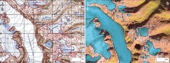
Fig. 2. (a) Geocoded topographic map (N50) from 1966 with digitized glacier outlines (red). Glacier outlines as derived from the 2006 Landsat scene are shown as an overlay (black). The distance between the gridlines is 1 km. (b) The same region in 2006 (composite with bands 5, 4 and 3 as red, green, blue; ice and snow is depicted in cyan) with glacier outlines from 1966 (white) and 2006 (black).
To calculate topographic inventory parameters (e.g. minimum, maximum, mean and median elevation, mean slope and mean aspect), the national digital elevation model (DEM) from the Norwegian mapping authority (Statens Kartverk) with 25m cell size was used. This DEM was derived from aerial photography, but the date of the photos varies within the study region and is thus unclear. This causes uncertainty in the derived inventory parameters, but it might still be acceptable for most of them, as the intermittent advance phase of many glaciers in the study region during the 1990s may have resulted in only small overall changes of the surface since that time. For the parameter minimum elevation, however, the differences from real values might exceed 50m and the values are accordingly less accurate.
The available hydrologic catchments (called regine in Norway) were slightly adjusted in some regions using a flow direction grid derived from the DEM and then used to separate contiguous ice masses into entities. For the comparison with the 1966 glacier extent, further adjustments to the basins were applied to fully include the 1966 extents but, at the same time, to exclude regions that were likely covered by seasonal snow in 1966. In total, nearly 300 glaciers were selected from this dataset for change assessment from 1966 to 2006.
For the inventory and change assessment we have used four Landsat TM scenes from 1997, 2003 and 2006. The two sequential scenes 201-16/17 (path-row) from 16 September 2006 were used for the new inventory and to derive area changes since 1966 (Fig. 2b), scene 200-17 from 15 August 1997 was used to determine cumulative changes in glacier length from 1997 to 2006, and a small part of the previously used scene 199-17 from 9 August 2003 gives area changes from 2003 to 2006. The 1997 scene was a raw image and orthorectified by NVE using 33 ground-control points. The 2003 scene was orthorectified and provided by the Centre for GIS and Earth Observation (Norsk Satellittdataarkiv). The 2006 scenes were ordered raw from the United States Geological Survey (USGS) and were orthorectified by NVE using 35 ground-control points. The quality of the georeference and orthorectification was tested against 14 check points. The processing was carried out with the OrthoEngine software from PCI Geomatica. The positional accuracy was better than 1 pixel (root-mean-square error (rmse)) for all images.
3. Data Processing
The original N50 map sheets from 1966 were scanned by the Norwegian mapping authority at 300 dpi and we geocoded them to Universal Transverse Mercator (UTM) zone 32 with ED50 datum). The achieved total rmse was 4.6–10m for the five maps. An attempt was made to obtain outlines from the geocoded maps with automatic pattern recognition, but as the glacier boundaries were drawn as dashed lines (Fig. 2a) the automated conversion to vector outlines failed. We therefore manually digitized the glacier outlines on the five selected N50 maps.
Multispectral classification of ice and snow from the Landsat TM images is based on the well-established band ratio method (threshold on TM3/TM5) with an additional threshold in TM1 to improve the classification in cast shadow (e.g. Reference Paul and KääbPaul and Kääb, 2005). All pixels with (TM3/ TM5) > 2.0 and TM1 > 40 were classified as being ice or snow. Selection of the TM1 threshold was rather difficult as the tongues of several outlet glaciers from the main ice cap were situated in deep shadow and poorly defined. However, the workload for post-processing of the converted glacier outlines was small compared with other regions, as there was generally little or no debris on the outlet glaciers and only a few regions had seasonal snow outside glaciers. A 3×3 median filter removed most of the noise in the classified glacier map, and remaining manual corrections were related to the deletion of misclassified lakes and adjustment of some calving glacier fronts.
After digital intersection of the drainage divides with the corrected glacier outlines, inventory parameters were calculated for each glacier entity (or zone) and the DEM using zonal statistics (cf. Reference Paul, Kääb, Maisch, Kellenberger and HaeberliPaul and others, 2002). The topographic parameters were calculated according to Reference PaulPaul and others (2009). For this purpose we also derived a slope and aspect grid from the DEM and calculated a mean aspect per glacier from the aspect values of all DEM cells within the specific glacier. For comparison with the 1966 glacier area, all separated parts in the 2006 scene were summed up within the extent of the 1966 entity, and the assigned size classes also refer to the 1966 extent.
Whereas the 2003 glacier outlines were taken from a previous study (Reference Andreassen, Paul, Kääb and HausbergAndreassen and others, 2008) ‘as is’, the 1997 TM scene was classified with the band ratio (TM3/TM5 > 1.7 and TM1> 60) and converted to outlines. Due to poor snow conditions, this scene could not be used to determine glacier area. However, most tongues from the larger outlet glaciers were well defined and snow-free and were used to assess length changes. For this purpose, a point at the 1997 and 2006 terminus near the central flowline was defined for each analysed glacier, and the Euclidean distance was measured in the GIS with a distance tool. We expect some deviations from field measurements of length change, as these have likely used reference points at different locations.
4. Results
4.1. Glacier inventory data
In the study region, we have compiled data for 1452 glacier entities larger than 0.01 km2 which cover an area of 993.5 km2. The count and area covered in selected size classes are listed in Table 1, and the percentages are depicted in Figure 3a. As in several other regions of the world, most glaciers in this region are small (79% are <0.5km2) and contribute little to the total area (12%), while a few large glaciers (1% are >10km2) add considerably to the total area (nearly 28%). When all glaciers smaller than 1 km2 are summarized in one class, all four classes cover about the same percentage (20–30%) of the total area. The 0.5–1 km2 size class is in the middle of the distribution, contributing the same percentage by number and area. The distribution of number and area by aspect sector reveals that 67% of all glaciers face the three sectors north to east (N, NE and E), while only 12% face the opposite quadrant south to west (S, SW and W) (Fig. 3b; Table 2). Compared with the number of glaciers, the contribution to the area covered is lower in the N to E quadrant (44%) and higher in the S to W quadrant (22%). This indicates that the N- to E-facing glaciers are much smaller than the S- to W-oriented glaciers. However, the largest individual contribution to total area comes from glaciers facing SE (23.5%), due to the dominant direction of the outlet glaciers emerging from the Jostedalsbreen ice cap (Fig. 1).

Table 1. Count (total number of glaciers) and area of all glaciers larger than 0.02 km2 in each size class along with their percentage of the total (see Fig. 3a)

Table 2. Count (total number of glaciers) and area of all glaciers larger than 0.02 km2 in each aspect sector along with their percentage of the total (see Fig. 3b). The rightmost column gives mean elevation in each aspect sector
When plotting mean glacier elevation vs aspect (full 3608 range), the clustering of most glaciers in the N to E quadrant is visible as well (Fig. 4a). Whereas glaciers facing the N sector have mean elevations of ~1455 m, the value is 1570m for glaciers facing S and SW (Table 2). Mean slope strongly decreases towards larger glaciers, and the scatter strongly increases towards smaller glaciers (Fig. 4b). For glaciers of the same size, mean slope can differ by a factor of two to three.
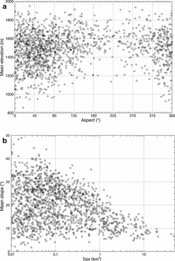
Fig. 4. (a) Scatter plot showing mean elevation vs aspect of all glaciers. (b) Scatter plot showing the relation between mean slope and glacier size.
The spatial distribution of mean elevation and mean slope is illustrated for the largest part of the analysed region in Figure 5a and b, respectively. As mean elevation is also a good proxy for the balanced-budget equilibrium-line altitude (ELA0) of a glacier (e.g. Reference Braithwaite and RaperBraithwaite and Raper, 2009), and a strong negative correlation between ELA and mean precipitation has been found (e.g. Reference Ohmura, Kasser and FunkOhmura and others, 1992), mean elevation is also closely related to precipitation amount. The strong precipitation gradient from the coast to the interior of Norway (e.g. http://met.no/English/Climate_in_Norway) can thus be clearly followed by the spatial distribution of mean elevation values (Fig. 5a): they gradually increase from low elevations (~700 m) on the ‘wet’ coast (shown in blue) to high elevations (up to 2000 m) in the drier interior (shown in red). There is a good correlation (r = 0.72) between mean glacier elevation and distance to an arbitrarily selected point in the southwestern corner of the study region (not shown). The spatial distribution of mean slope values in Figure 5b indicates a close relationship between glacier type and mean slope. Whereas glaciers related to ice caps or compound glaciers have generally low mean slopes, the values are much higher for most cirque and mountain glaciers.
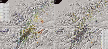
Fig. 5. (a) Colour-coded visualization of mean elevation (only glaciers larger than 0.5 km2 are considered) on a hillshade of the DEM with glacier areas in dark grey. The legend gives values in metres. (b) Same as (a), but for mean slope. The legend gives values in degrees.
The area–elevation distribution depicted in Figure 6 reflects a combination of ice caps with normal mountain and valley glaciers. Whereas the distribution of the former is biased towards higher elevations (e.g. Reference Paul and AndreassenPaul and Andreassen, 2009), the latter is more normally distributed. In this region most of the ice is found in a small elevation band between 1400 and 1800 m, with a peak at 1600 m, indicating high sensitivity to changes in the ELA and thus to climate changes (e.g. Reference Nesje, Bakke, Dahl, Lie and MatthewsNesje and others, 2008). The same is true for glaciers smaller than 1 km2 and the Jostedalsbreen ice cap itself (with its three main domes). Glaciers smaller than 1 km2 have an evenly shaped hypsometry with a maximum at 1500 m.

Fig. 6. Area–elevation distribution for different glacier samples in 10m bins.
4.2. Change assessment
The relative change in area since 1966 for a subsample of 297 glaciers (1966 extent) is visualized in Figure 7 and listed in Table 3 for individual size classes. Most glaciers have lost area since 1966, but a few, mostly small glaciers are larger in 2006. The scatter of change values strongly increases towards smaller glaciers and there is a trend to stronger relative area loss with decreasing glacier size. However, the mean value for several size classes is similar for all glaciers larger than 5 km2 (around –5%) as well as all glaciers smaller than 0.5 km2 (around –40%). In the mean, the area loss is 9% (or 67.4 km2) for this sample, with glaciers smaller than 1km2 and glaciers larger than 10km2 contributing about equally to the total loss (29% and 25% respectively). The area of Jostedalsbreen itself has changed from 520 km2 in 1966 to 488.5 km2 in 2006 (–6.4%), with 13km2 now detached from the main ice mass. Due to the close relation of glacier size and relative area change, the geographical distribution of the change also shows a distinct pattern: it is higher in regions with smaller glaciers, and the converse.
Table 3. Area changes per size class from 1966 to 2006 for the subsample of 297 glaciers

Fig. 7. Scatter plot showing the relative change in glacier area (1966–2006 period) vs glacier size (see Table 3).
The comparison of glacier sizes in 2003 and 2006 for a selection of 83 glaciers (in 2003) revealed an overall area loss of 9.5% in this period. At Harbardsbreen, for example, the 2003 outlines are clearly outside the 2006 outlines (Fig. 8a), indicating area loss along the entire perimeter (totalling 1.55 km2, or 5.9%). This pattern of change can also be observed for most other ice caps in the sample, i.e. for this glacier type a locally small retreat of one or two pixels sums up to comparably large overall area losses. When converting the 3 year loss to a mean value per year (3.2%) and comparing it with the mean value in the same size classes (0.05–10km2) for the 1966–2006 period (0.33%), an acceleration of the area loss by a factor of ten can be derived. However, considering that locally some seasonal snow might have been attached to the glaciers in 2003, this mean area loss rate is likely an upper bound.
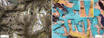
Fig. 8. (a) Overlay of glacier outlines from 2003 (yellow) as derived from the neighbouring TM scene (Reference Andreassen, Paul, Kääb and HausbergAndreassen and others, 2008) and from 2006 (black) from the scene analysed here (also shown in the background) for the region around Harbardsbreen (HB). (b) Changes in glacier length between 1997 (white lines) and 2006 (black) for the northeastern dome of Jostedalsbreen. The inset is a close-up of the terminus from Stegaholtbreen (see Table 4). A large new lake formed at Erdalsbreen (ED).
Cumulative length changes from 1997 to 2006 were compared with field measurements for nine glaciers (Table 4). From this sample, the field measurements show that five glaciers changed between –105 and –420 m, while for four glaciers the changes ranged from –40 to +17 m. Considering an uncertainty of ~1 pixel for satellite measurements, it is not expected that the latter are identifiable. However, the close-up of Stegaholtbreen (Fig. 8b) shows that a 1 pixel change in length can be visible under good conditions. Of the five glaciers with the largest changes, agreement with the satellite-derived values is good for three of them, while larger deviations occur for the other two. This is likely due to the terminus being located in cast shadow which results in higher uncertainty. Though these deviations have little impact on the accuracy of the total glacier area, they clearly demonstrate the limitations of spaceborne length-change measurements. Nevertheless, digital overlay of both outlines allowed us to analyse length changes of many more glaciers in the region. For example, in the southern part of Jostedalsbreen (Fig. 9) we found a 550m retreat of Langedalsbreen, a 300–500m retreat of an unnamed outlet glacier north of the Kaldekari rock outcrop (arrow) and a ~700m retreat of Boyabreen. In the north, the tongue of Erdalsbreen retreated 750m and was replaced by a lake (Fig. 8b). These findings show that fluctuations of unmeasured glaciers can be even stronger than those of measured ones and emphasize that it is worthwhile to determine length changes from satellite data for a larger sample of glaciers to obtain a more representative overall picture.
Table 4. Comparison of cumulative length changes (1997–2006) for nine outlet glaciers of the Jostedalsbreen ice cap. ‘No.’ refers to table 2 in Reference Andreassen, Elverøy, Kjøllmoen, Engeset and HaakensenAndreassen and others (2005), ‘In situ’ and ‘Satellite’ give the measured length change in metres, and ‘Diff.’ gives differences between field and satellite measurements in units of a sensor pixel (30 m)
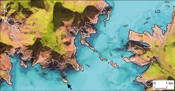
Fig. 9. Changes in size and length (yellow lines) of various unmeasured glaciers in the southwestern part of Jostedalsbreen between 1997 (white) and 2006 (black). The outlet glacier Langedalsbreen (LD) and the Kaldekari rock outcrop (arrow) are marked.
5. Discussion
5.1. Data availability
In several maritime regions of the world the availability of Landsat scenes with appropriate conditions for glacier outline mapping is limited and periods without usable scenes may be longer than 5–10 years in some regions. In addition to cloud conditions on the day of the satellite overpass, seasonal snow is the main hindrance to obtaining useful satellite data. Years with very negative mass balances likely provide the best glacier-mapping conditions. It can thus be speculated that there is a (negative) correlation between the number of useful Landsat scenes and the health of glaciers in a specific region. A strong improvement of the repeat interval will occur when the Landsat Data Continuity Mission (LDCM) and Sentinel 2 sensors are in operation. Furthermore, with increasing global temperatures in the future (e.g. Reference Nesje, Bakke, Dahl, Lie and MatthewsNesje and others, 2008), the problem with seasonal snow might be reduced, unfortunately at the expense of rapidly shrinking glaciers.
5.2. Drainage divides
Classifying glaciers in this region dominated by ice caps, and thus with only a few debris-covered glaciers, was straightforward. The entire processing including threshold selection and editing (lakes, shadow) was accomplished within a few hours. The more demanding issue in this region was defining drainage divides on ice caps. One challenge is the DEM accuracy in flat accumulation regions with low optical contrast on either satellite imagery or aerial photography (e.g. Reference Racoviteanu, Paul, Raup, Khalsa and ArmstrongRacoviteanu and others, 2009; Reference Bolch, Menounos and WheateBolch and others, 2010). This introduces some uncertainty to the derived glacier area for individual glacier entities (Reference Le Bris, Paul, Frey and BolchLe Bris and others, 2011). Moreover, differences in drainage divides give a variation in area for different inventories. Whereas it is necessary to separate an ice cap into its drainage basins when regional hydrology is the purpose, ice caps need to be treated as a whole for glaciological (e.g. flow modelling or volume calculations) or climatological purposes (e.g. change assessment). It can thus be concluded that the glacier area of individual outlets and the number of glacier units are rather ‘ill-defined’ and should only be used in glaciological applications after careful analysis.
5.3. Inventory data
Accuracy
As the accuracy of the mapped glacier outlines is difficult to assess when an appropriate ground truth is not available (e.g. Reference Svoboda and PaulSvoboda and Paul, 2009), we refer here to the results of previous studies (e.g. Reference Paul, Huggel, Kääb, Kellenberger and MaischPaul and others, 2003; Reference Andreassen, Paul, Kääb and HausbergAndreassen and others, 2008) and estimate that the overall accuracy of the satellite-derived glacier area for the comparably clean glaciers in this region is better than 5%, with glacier-specific values up to 5–10% (e.g. for glaciers located in cast shadow). Of course, this estimate does not consider uncertainties in area for individual units related to the position of the ice divides. From a manual multiple digitizing experiment performed for 30 smaller glaciers in the same region, we found good agreement with the automatically derived glacier areas. However, the variability of the manually digitized areas was higher (the range of the mean differences was 5–10%) than the estimated error (better than 5%) of the automatically derived outlines. Though the manual digitizing might be superior in including mixed pixels that might not be included in the automatically derived outlines, the latter have the advantages of being more consistent and reproducible throughout an entire scene, and of course much faster to derive.
Topographic parameters
To derive topographic inventory parameters, we used a DEM compiled from aerial photography acquired up to 20 years before the satellite image. As Reference Frey and PaulFrey and Paul (in press) have shown for the Swiss Alps, this likely has a small influence for most of the parameters that are averaged over several thousand pixels (e.g. mean elevation, slope or aspect). In times of rapid terminus changes, however, minimum elevation should better refer to a more up-to-date DEM, so we analysed the suitability of the Advanced Spaceborne Thermal Emission and Reflection Radiometer (ASTER) global DEM (GDEM) for this purpose. However, we found too many artefacts in the GDEM close to the termini and thus decided to use the national DEM. In the case of retreating glaciers we now have too high values for minimum elevation as the terminus is located on the former glacier surface. This should be corrected once a more recent and suitable DEM becomes available.
Data analysis
The histograms of glacier number and total area in regard to glacier size classes confirm earlier studies that show similar distributions (e.g. Reference Paul and AndreassenPaul and Andreassen, 2009; Reference Bolch, Menounos and WheateBolch and others, 2010). Though glaciers smaller than 1 km2, and particularly less than 0.1 km2, contribute little to the total area covered, they provide most of the glaciers by number and contribute significantly to the total area change (20% in this case). Applying automated mapping techniques rather than manual delineation is therefore recommended in order to include the entire sample. That most of the glacier area in this region comprises glaciers facing SE is due to the dominant role of the Jostedalsbreen ice cap with its outlet glaciers and the specific topographic conditions (SW–NE ridge). The dominance of northerly aspects as found in other regions (Reference EvansEvans, 2006) is thus only visible for our sample in the number of glaciers rather than in the area covered. A weak dependence of mean glacier elevation on mean aspect was found, but the scatter is very high (Fig. 4a) and the dependence on distance from the coast is much clearer (Fig. 5a). The latter dependence has been found in earlier studies (e.g. Reference Østrem, Selvig and TandbergØstrem and others, 1988; Reference Lie, Dahl and NesjeLie and others, 2003).
5.4. Change assessment
A direct comparison with the previous inventory (Reference Østrem, Selvig and TandbergØstrem and others, 1988) has not been made as the position of the used drainage divides will undoubtedly be different and the previous basins are difficult to reconstruct. The obtained glacier changes from 1966 (maps) to 2006 do have uncertainties due to assumed adverse snow conditions, in particular for the northern map sheets (1418-IV). This is deduced from the very patchy pattern of the outline (Fig. 2a) that was similarly found in other regions. As the N50 maps were created by cartographers rather than glaciologists, in general the maps do not distinguish between seasonal or perennial snow and glaciers (Reference Paul and AndreassenPaul and Andreassen, 2009). This may result in too large glacier areas and hence too strong area losses since 1966. We have tried to account for this by partially adjusting the 1966 extents for obvious seasonal snowfields and excluding very unclear cases from the analysis. On the other hand, the positive area changes found for some of the smaller glaciers might also result from seasonal snowpatches that still existed in the 2006 scene. Seasonal snow can also be an issue for the high loss rates in the 2003–06 period (e.g. yellow outlines in Fig. 8a that do not have a black line inside), but the area loss along the entire perimeter (where the ice is thinnest) hints at a strong downwasting of the larger ice caps and their very sensitive reaction to small climatic changes (e.g. Reference PeltoPelto, 2010). We conclude that the area-change values derived here for both periods represent upper bounds, especially for smaller glaciers.
Regarding the assessment of cumulative length changes from satellite observations, we identified larger differences with respect to field observations when a glacier terminus is located in cast shadow, but found good agreement with field observations for the other glaciers (~1 pixel). As the results of such a direct comparison are also influenced by methodological differences, for example when different lines of sight are used (cf. Reference Hall, Bayr, Schöner, Bindschadler and ChienHall and others, 2003), we conclude that the good agreement found here is promising and can be suggested for a more extended application (see Fig. 9). From the more qualitative analysis (visual inspection) of the changes we conclude that not all outlet glaciers of Jostedalsbreen advanced from the 1980s to 1997, and not all of them retreated from 1997 to 2006. Instead, there is a high variability in the activity of individual outlets, and results from the field measurements cannot be generalized to the entire ice cap.
6. Conclusions
We have presented results of a new glacier inventory of the Jostedalsbreen ice cap derived from two Landsat TM scenes from 2006 and a national DEM with 25 m spatial resolution. In a hydrologic sense, we created inventory data for 1452 entities, but many of them are related to compound glaciers or ice caps so that the total number of glaciological entities is smaller. Changes in glacier size from 1966 and 2003 to 2006 were derived for 297 and 83 glaciers, respectively, yielding a high spatial diversity, an overall area loss of 9% since 1966, and glaciers smaller than 1 km2 contributing about one-third to the total loss. Jostedalsbreen as defined here shrank from 520 km2 in 1966 to 488 km2 in 2006 (6.4%). A strong acceleration of the area loss for the recent past (2003–06) by a factor of ten is observed, but this might be due to the extreme 2006 ablation period. The comparison of cumulative length changes for nine outlet glaciers (1997–2006) revealed promising agreement with the field measurements (by ~1 pixel in most cases). Compared to the latter, even stronger changes were found for some non-measured glaciers. Whereas optical satellite imagery provides the most efficient means to assess overall changes at a regional scale, cloud and snow conditions are critical constraints for their availability. Thus, field-based observations are still mandatory to record annual glacier fluctuations, but satellite data are most useful to record changes at a larger scale and over longer time periods. Satellite scenes with adverse snow conditions might still be useful for assessing length changes, at least for larger outlet glaciers.
Acknowledgements
J.E. Hausberg is thanked for orthorectifying the 1997 and 2006 satellite images. This work was supported by internal funding by NVE and external funding by Statkraft SF, and the European Space Agency projects CryoClim and GlobGlacier (21088/07/I-EC). We thank T. Jóhannesson and an anonymous reviewer for constructive comments.