


Introduction
The flow of the ice sheet leading to the deep-drilling site at Dye 3 has been studied on both a large scale and a small, more detailed scale. The detailed study area, discussed here, is located within the eastern cluster of the large-scale network of observation points and is situated immediately up-glacier of the drill site (Fig.1). The special feature of the detailed network is the closely spaced series of observations of surface velocity, accumulation rate, ice thickness, and internal layer depth carried out along three parallel lines. Certain results from the large-scale study for ice movement (Reference Drew and WhillansDrew and Whillans 1984), firm stratigraphy, temperature and snow accumulation (Reference BowBow in press), and radar sounding (Reference Jezek, Roeloffs and GreischerJezek and others in press, Reference Overgaard and GundestrupOvergaard and Gundestrup in press) are also used here.

Fig. 1 Southern Greenland. The detailed strain network is south-west and up-glacier from Dye 3.
The detailed program is designed to support the interpretation of the results from the deep drilling and to describe the manner by which the ice sheet negotiates hills and valleys in the bed. The latter is the subject of the present report. We find that, at the surface, the flow is much less complex than anticipated, and that lateral flow variations are much less important than longitudinal variations. At depth, however, the story is mixed: there are two sites where the flow is not simple, but for large-scale features on most of the strain network the data are consistent with flow at depth being in the same direction as flow at the surface.
In this regard a distinction is made between planar and non-planar flow. In planar flow the velocity vectors along a vertical column through the ice sheet all lie in a single plane but simple third-dimensional convergence or divergence is allowed. Non-planar flow involves deep ice travelling in different directions than shallow ice.
The Data
A map view of the detailed strain network is shown in Figure 2(a). Data were collected along three rows, labelled A, B and C, about 2 km (one ice thickness) apart. Movement is left to right in the figure and each dot represents the site of a velocity determination; these are summarized in Table I. The Dye 3 bore hole is near station 81 (Table I). The network contains stations 3003 (at A1) and 3005 (between A11 and A12) of the large-scale study, and satellite-determined movements of these stations provide absolute velocity and orientation reference. Relative movements within the detailed network were obtained by repeated trilateration using Hewlett-Packard Model 3808A electronic distance meters and a subsequent simultaneous least-squares solution for coordinates.

Fig. 2 Map presentations of velocity, radar results, and velocity gradient along the detailed strain network. Flow is from left to right and Dye 3 is at station B1.
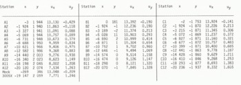
Table I Coordinates in 1980 (m) and Horizontal-Velocity Components (m a−1)
Velocity gradients are plotted in Figure 2(e) to (h) and, based on manufacturer’s specifications and field conditions, should be accurate to 1 or 2 × 10⁻⁵ a−1. As indicated in Reference Drew and WhillansDrew and Whillans (1984) there is an unexplained discrepancy with the satellite-determined length of the strain network but the disagreement is, at most, equivalent to 3 × 10⁻⁵ a−1 if distributed over the entire network, and does not affect the interpretation here.
Radar depth sounding of bottom topography was carried out along the detailed strain network and continuous profiles were recorded using 35 and 60 Wz radars operated on the surface (Reference Jezek, Roeloffs and GreischerJezek and others in press and Reference Overgaard and GundestrupOvergaard and Gundestrup in press). Data were also collected along a line used by investigators from the State University of New York at Buffalo: that line is shown by the dots running at an angle to the three lines of the strain network. The bottom topography presented in Figure 2(d) is derived primarily from the 35 MHz data with supplementary interpretation using gravity data and is broadly compatible with the results of the 60 MHz radar survey. The precision of both radar surveys is about ±15 m, but at a few locations near the bore hole the relative difference between bed elevations from the two data sets is 100 m. The large difference is primarily due to a reduction in the strength of the radar signal in the region about 5 km up-glacier of Dye 3, where much of the interpretation relies on a combination of radar and gravity data.
Radio-reflecting horizons internal to the ice sheet were also recorded on the continuous profiles and the elevation of one of these is shown in Figure 2(c). The precision of these measurements is also about ±15 m. There is no apparent difficulty in tracing the radar layer along the A, B, and C lines or between A1 and C1 or A12 and C12.
Surface elevations (Fig.2(b)) were measured by hand-held pressure altimeter referred to the satellite tracking stations. Station A1 is also station 3003 in Reference Drew and WhillansDrew and Whillans (1984) and its elevation is 2 490 m a.s.l. The contours are least accurate farthest from Dye 3, where the error may be ±2 m.
Accumulation rates were determined from measurements of gross-beta activity associated with nuclear explosions (Reference BowBow in press) and from repeated measurements of heights of bamboo poles. The first technique provides long-term averages for a few sites and the second detects short-distance variations more satisfactorily. The accumulation rate at A12 is 0.444 Mg m−2 a−1. No systematic short-distance variations were detected. The variations suggested by Reference Reeh, Johnsen and Dahl-JensenReeh and others (in press) for this region are smaller than the variability of the data obtained with bamboo poles.
Flow Pattern
Surface velocity vectors (Fig.2(a)) are nearly parallel to one another and show a turning to the right. From one end of the network to the other, velocities increase about as expected for balance with the net surface snow accumulation, although there are local exceptions as discussed below.
The bed (Fig.2(d)) is characterized by several irregularly-shaped knolls separated by deep valleys striking to the north and south. In general, the topography under the strain network is less rugged than the terrain farther up-glacier and nearer the ice divide (Reference Jezek, Roeloffs and GreischerJezek and others in press). Numerous diffraction hyperbolae observed on the flanks of the hill hill near B5 suggest that the bottom is rough on a scale of several tens of meters. The ice thickness varies by as much as 20% within the strain network.
As has been generally found elsewhere, the surface elevation (Fig.2(b)) drops in steps over the basal highs (Fig.2(d)) with the steepest surface slopes where the ice is thinnest; good examples are found between B10 and B9 and between B5 and B4.
The flow along the strain network is generally longitudinally extensive (Fig.2(e)). This is in accordance with near-parallel flowlines and progressively faster flow needed to export the net snow accumulation.
Locally the longitudinal strain-rate varies between near zero and twice the average. The ice stretches more on the approach to basal obstructions, and the variations in longitudinal velocity are roughly proportional to variations in ice thickness, but of opposite sign. Such a relationship is necessary between mean velocity and ice thickness to maintain continuity in ice flux. It is significant that the relationship also applies for surface velocity. This indicates that, at depth, divergence around or convergence between obstacles is not important to the overall ice flux. Also, because surface velocities vary as mean velocities, most of the shear must be in deep layers. Thus the flow appears to be planar and the main thickness moves almost as a block. This conforms to generally accepted theory and is as found near Byrd station, Antarctica (Reference WhillansWhillans 1977).
At the surface, flow and flow variations in the lateral direction are much weaker than those in the longitudinal direction. The pattern of lateral strain-rate (Fig.2(f)) nevertheless shows divergence on the approach to the ridge between C6 and B5 and lateral convergence into valleys located at A1, A3, and A7. This is as normally expected for flow avoiding highs and favoring valleys, but the effect is weak. At the up-glacier end of the network, the lack of lateral divergence approaching the hill at B10 is unexplained. The convergence between B12 and C12 may be associated with flow in the lee of a basal high reported by Overgaard and Gundestrup just up-glacier (not shown on our map).
The velocity gradients ∂ux/∂y contrast longitudinal variations of neighboring flowlines. There is an average shear such that flow along the C-line is faster than along the A-line. Superimposed on this are local variations indicating that velocities are higher where the ice is thin than they are where the ice is thicker. This is in the expected sense to maintain volume flux. There is no tendency for “streaming”, which would be the opposite effect, in which ice in valleys would travel faster and follow the axes of the valleys.
The final set of velocity gradients, ∂uy/∂x (Fig.2(h)), shows deflection of the flowline by basal obstacles. The deflection is to the right and is also clear in the turning of the velocity vectors (Fig.2(a)). These gradients can be combined with ∂ux/∂y to show east-west stretching: where
 is large, ice on the right-hand flowline is passing over a basal high first, accelerating, and pulling neighboring ice with it. The effect is small. (Similar gradients near −20 km are calculated for a coordinate system aligned with the velocity vectors rather than the x-axis.)
Summarizing the velocity data, we find that most velocity variations are along the flowline. That is, gradients of uy, in our coordinate system, are much less than those of ux. Presumably variations in ux dominate because it is this, the main component of flow, impinging on basal features that leads to all flow variations. Nonetheless it is surprising that lateral variations in bottom topography have so little influence on ice flow at the surface.
To examine whether this condition persists with depth we study an internal radio-reflecting layer buried to about 1 000 m depth (Fig.2(c)). Internal layers are often taken to be isochrones. If so, the shape of the layer should be indicative of flow at depth. Elsewhere the layers have been found to mimic the bottom topography (Reference Robin, Evans and BaileyRobin and others 1969, Reference WhillansWhillans 1977, Reference Whillans and JohnsenWhillans and Johnsen 1983), although the shape of the layer is generally much smoother. In central East Antarctica, however, Reference Robin and MillarRobin and Millar (1982) found sites where the layering does not mimic the bottom but shows much more complex features, or is absent. They interpret this to indicate flow around obstacles in the bed.
Figure 3 shows the topographic maps of Figure 2(b), (c) and (d) with regional gradients removed in order to display better the relations between local variations. The data show the internal layer following the bed in most places. For example, there are hills at B5 and valleys at B7 in both bed and internal layer with the internal-layer relief being about 25% that of the bed. At this site the damping is isotropic: the ratio of internal layer to bed relief is about the same in both longitudinal and lateral directions. This is also true at the surface (Fig.2(b)) where there are important lateral slope variations. It is as if the bed relief were simply damped and, in the case of the surface, phase-shifted up-glacier. The damping is due to faster flow over obstacles and consequent longitudinal stretching and vertical thinning of the ice between the internal layer and the bed. If there were changes in flow direction at depth (non-planar flow) ice would be advected under or away from under the surface flowlines, and the internal layer would not correlate with the bed beneath it. Similarly, if ice in some of the valleys were nearly stagnant then these sites would be identified by an anomalously high internal layer. The correlation is, in many places, strong, albeit not perfect, and planar flow describes adequately the major part at these sites.

Fig. 3 Data for Figure 2(b), (c), and (d) with regional slopes removed (slopes of 0.004, 0.007, and 0.025 removed, respectively).
There are, however, two locations where the internal layer has a form very different from the bed. The basal hill at B10 and B9 has almost no corresponding expression in the internal layer. There the contours of internal-layer elevation are nearly perpendicular to the contours of bottom topography. There is a weak influence of the bed in cross-section (Fig.4) but it is subdued compared to the rest of the survey. The narrow subglacial valley near the down-glacier end of the survey is the second example, but this is more easily understood because the valley is a much smaller feature than the hill near B9 and B10.

Fig. 4 Profile along B-line. Solid and dashed lines are from 35 MHz radar. Dashed bed represents bottom reflections obtained on a line = 100 m to the south-east of B-line. The deepest internal layer is also shown in Figure 2(c). All layers show the same pattern of deformation. Open dots at bed are results from the 60 MHz radar.
If the proposition that the internal layer follows an isochrone is maintained, then these data indicate that flow at depth is different from that at the surface. This could be because of stagnant ice near the bed (Reference Colbeck, St Lawrence and GowColbeck and others 1978, Reference Russell-Head and BuddRussell-Head and Budd 1979: 126) or because of changes In lateral convergence or divergence with depth at these sites.
According to the first suggestion of nearly stagnant ice, there would be an apparent ice bottom that is smoother than the bed. However, surface velocity variations (Fig.2) up-glacier from B10 seem to follow closely the changes in the bed and not a smoother effective bed. It seems that there the ice below the anomalous internal layer participates normally in ice flow and is not nearly stagnant. Relatively stagnant ice in the valley from C2 to A1 remains a possibility, however.
Support for more stagnant ice near the bed near Dye 3 comes from the observation of silty ice in the lower 50 m of the Dye 3 core whose sedimentary stratigraphy is not well developed compared to the ice above (Reference DansgaardDansgaard and others 1982). If that interpretation is correct then this ice is not part of the main flow of the glacier, and is much older than the ice above. The valley is narrow, and models of the influence of bed variations on ice flow (for example, Reference Whillans and JohnsenWhillans and Johnsen 1983, Reference Reeh, Johnsen and Dahl-JensenReeh and others in press) indicate that short wavelength features affect flow only near the bed.
For the anomalous site up-glacier from B10 we favor the suggestion that lateral convergence or divergence changes with depth (non-planar flow). Perhaps at depth near A10 there is more lateral convergence of flowlines than near the surface. Then, because ice is incompressible vertical thinning of deep ice would be anomalously small and a layer of given age would be anomalously high above the bed. Such behavior is more probable near the ice divide where the flow is less directed. Farther down-glacier, where the flow is more consistent, such anomalous ice from near the ice divide is drawn out and thinned, and so is not evident in our study.
Interpretation
This qualitative description of ice flow over a rugged terrain provides insight into the interaction of the ice sheet with its bed. The terrain is rough, showing changes of 400 m in distances of 2 km, but the flow seems to be comparatively simple.
The flow variations are mainly in the longitudinal direction at the surface and apparently also at depth. Effects of important non-planar flow (in which velocity vectors change geographic direction with depth) are not evident for major features over most of the network.
Flow around obstructions (non-planar flow) must certainly be important very close to the bed, but it seems that the main body of the glacier reacts only to large-scale features in the direction of flow (the wavelength of variation at the surface is S to 8 km, or 2.5 to 4 times the ice thickness). Neighboring flowlines vary according to their separate bed forms and are not greatly influenced by topography to the sides. This differs from flow in a floating ice shelf where drag at the walls or around islands dominates. Near Dye 3 the flow is affected mainly by obstructions directly beneath the flowline.
Overall, the glacier has adjusted to basal obstructions by building slightly in thickness behind them. This causes steeper slopes over obstructions. In a manner analogous to water flow over a weir, the glacier accelerates on the approach to the thinner region.
The mechanistic link between surface, bed topography and speed variation involves changes in shear stresses on horizontal planes. According to the standard formula, shear stresses are larger where slopes are steeper. These larger stresses lead to the faster flow needed to pass the ice flux through the reduced thickness.
An equivalent description of this process has been applied to related data near Byrd station, Antarctica (Reference Whillans and JohnsenWhillans and Johnsen 1983). In that description the glacial surface is viewed as being higher than average behind an obstruction. The extra weight causes extra horizontal stretching of the glacier and faster velocities over the obstruction. Short wavelength basal features have little gross effect.
The forms of the internal layer over the narrow valley near the core hole and at the up-glacier end of the network do not correlate with the bed. The narrow valley is only weakly apparent in the internal layer or in surface topography or strain-rate: presumably ice in the valley does not fully participate in the main flow (as predicted by theory assuming planar flow). At the second special site, near B12, the anomalously high internal layer indicates extra relative thickening of the ice below it. There are no special features in the bed up-glacier of this site (Reference Overgaard and GundestrupOvergaard and Gundestrup in press) that can explain such behavior, but the site is only ten ice thicknesses from the ice divide, and flow near ice divides is less well-directed (less planar) than farther down-glacier.
The different behavior near B12 is attributed to its proximity to the ice divide, but the most pronounced three-dimensional feature under the network is the hill, also situated there. The other hills are ridges aligned diagonally to the flow. Perhaps the flow is everywhere more complex than the data seem to suggest but the diagonal ridges and valleys cause flow that appears more simple than it is.
The data are too limited in extent to determine whether planar or non-planar flow dominates in this part of Greenland. The planar-flow model works well near Byrd station (Reference Whillans and JohnsenWhillans and Johnsen 1983) but not in certain places in East Antarctica (Reference Robin and MillarRobin and Millar 1982), Near Dye 3 it describes long wavelength features for the 15 km nearest to the core hole, but not features between 15 and 20 km.
We thank Richard Alley for very valuable help and discussions. This work was supported by National Science Foundation grant nos. DPP-8008356 and 8306689.


