


Introduction
Ice algae are an integral component of the Arctic ice-covered marine ecosystem, where they provide an important initial food source for early spring grazers (e.g. Reference Bradstreet and CrossBradstreet and Cross, 1982; Reference HornerHorner and others, 1992; Reference Leu, reide, Hessen, Petersen and BergeLeu and others, 2011). In recent decades, the Arctic marine environment has experienced numerous changes, including earlier melt onset (Reference Markus, Stroeve and MillerMarkus and others, 2009), shrinking and thinning of multi-year sea ice (MYI) and a transition from MYI to predominantly first-year sea-ice (FYI) cover (Reference StroeveStroeve and others, 2012). These changes in algal habitat will influence ice algae abundance and productivity. For example, an earlier melt onset can shorten the ice algal bloom period (Reference Campbell and GosselinCampbell and others, 2014), whereas a change from multi-year to first-year ice cover could favour higher ice algal production (Reference Arrigo and MockArrigo and others, 2010). However, we lack a sufficiently detailed understanding of the ice-covered ecosystem to quantify its actual response to the changing environment with any certainty. In particular, there is a deficit of spatial and temporal observations of ice algae and their environment across the Arctic (Reference Arrigo and MockArrigo and others, 2010). This paucity of data is partially due to logistic and methodological challenges (Reference Nicolaus, Katlein, Maslanik, Hendricks, Palmisano and SooHooNicolaus and others, 2012), as well as the destructive nature of most conventional ice algae sampling methods (Reference Mundy, Ehn, Barber and MichelMundy and others, 2007).
Multiple studies have demonstrated a significant influence of ice algal biomass on the spectral distribution of light underneath ice covers (Reference MaykutMaykut and Grenfell, 1975; Reference ArrigoArrigo and others, 1991; Reference Legendre and GosselinLegendre and Gosselin, 1991; Reference Perovich, Cota, Maykut and GrenfellPerovich and others, 1993; Reference Mundy, Ehn, Barber and MichelMundy and others, 2007; Reference Fritsen, Wirthlin and MombergFritsen and others, 2011). Absorption by algal pigments decreases the transmitted light, while acting to shift and narrow its spectral distribution from a broad peak centred at ∼460 nm under an ice cover with little algal biomass to a sharp peak centred at ∼570nm under high ice algal concentrations (Reference Mundy, Ehn, Barber and MichelMundy and others, 2007). In turn, this modification of transmitted light is likely to feed back and affect ice algal growth (Reference HornerHorner and Schrader, 1982; Reference Grossi, Kottmeier and MoeGrossi and others, 1987; Palmisano and others, 1987). Comprehensive knowledge of the ice cover’s optical characterization is therefore essential to improve our understanding of the Arctic marine ecosystem, especially considering the expected impact of observed sea-ice changes on light transmission (Reference Nicolaus, Katlein, Maslanik, Hendricks, Palmisano and SooHooNicolaus and others, 2012).
Numerous efforts have been made to quantitatively describe the optical properties of ice covers. Many of these make use of radiative transfer models (e.g. Reference Fritsen and AckleyFritsen and others, 1998; Reference Hamre, Gerland and StamnesHamre and others, 2004; Reference PerovichPerovich, 2005). While these models may be used effectively for purposes such as analysing spatio-temporally varying ice covers (Reference PerovichPerovich, 1990) and estimating algae’s effect on transmittance (Reference GrenfellGrenfell, 1991), they are limited by their requirement of a priori knowledge of an ice cover’s qualitative characteristics. Recently, Reference Nicolaus, Katlein, Maslanik, Hendricks, Palmisano and SooHooNicolaus and others (2012) produced an Arctic-wide map of light distribution under summer sea ice, using a combination of satellite data and measurements from a remotely operated vehicle (ROV). Their approach allowed for large-scale estimations of light transmission through different types of ice and surface covers without a heavy dependence on assumptions and parameterizations, and was used to make predictions about the changing nature of the Arctic light environment. However, it could not be used to describe the ice cover’s optical properties on the microscale, nor did it account for the spectral distribution of transmitted light. Other attempts to characterize ice covers have involved direct calculation of spectral attenuation coefficients. For instance, Reference Perovich, Cota, Maykut and GrenfellPerovich and others (1993) calculated a biomass-specific diffuse attenuation coefficient for algae by comparing transmitted irradiance beneath an ice cover before and after removing the bottom algal layer. Light and others (2008) derived spectral extinction coefficients for ice from irradiance profiles using a finite-difference formula. These direct methods allow more flexibility than radiative transfer models, but require a range of additional measurements. For instance, in the work of Light and others (2008) irradiance profiles had to be taken every 0.10m within boreholes through the ice.
In this paper, we consider the spectral optical depth of Arctic sea ice. The spectral optical depth, denoted τ(λ), is a dimensionless, wavelength-dependent parameter that describes the attenuation of light at wavelength λ as it passes through a medium and can be given by
where Ed,top(λ) and Ed,bot(λ) are the downwelling incident (on top of the snow-ice cover) and transmitted (below the bottom ice algal layer) spectral irradiances (W m–2 nm–1 )
, respectively. For Arctic first-year snow-covered sea ice, the main components of light attenuation during the spring algal bloom are ice algal biomass, snow depth and sea-ice thickness (Reference Perovich, Roesler and PegauPerovich and others, 1998), although sediments and other absorbing constituents (e.g. soot) can also play an important attenuation role in specific areas of the Arctic (Reference Light, Grenfell and PerovichLight and others, 2008). Because of the strong dependence of attenuation on algae, snow and ice, a functional model can be used to describe optical depth at specific wavelengths as a function of these main attenuating components.
To create such a model, we used a statistical technique from the field of functional data analysis (FDA). FDA is the extension of traditional statistical methods, such as multiple linear regression and significance testing, to data that are curves over a domain, such as time or wavelength (Reference Ramsay and SilvermanRamsay and Silverman, 2005). The main goal of FDA is to consider discrete measurements of these curves and to describe the underlying smooth functions from which the measurements originated. FDA techniques have been successfully applied in various fields, such as medicine (Reference Sørensen and GoldsmithSørensen and others, 2013), psychology (Reference Vines and KrumhanslVines and others, 2006) and biology (Reference Müller, Wu and DiamantidisMüller and others, 2009).
Here we consider functional linear regression where the response variable is a smooth function and the covariates can be scalar or functional. We used discrete measurements of incident and transmitted irradiance to create smooth representations of optical depth as a function of wavelength. A functional linear regression model was then developed using optical depth as a functional response. Chlorophyll a (chl a) concentration (a commonly used proxy for algal biomass), snow depth and ice thickness were used as scalar covariates. In this case, the regression coefficients were also smooth functions of wavelength.
The utility and uniqueness of our approach is a result of its entirely data-driven nature. Using only measurements of irradiance and the aforementioned covariates, our model estimated spectral attenuation coefficients for the entire ice cover without any prior assumptions about its composition. Thus, it provides a relatively simple and computationally inexpensive way to analyse the optical properties of sea ice. FDA methods, such as those described here, may therefore facilitate improved understanding of the Arctic marine ecosystem.
Methods
Data collection
Field data were collected on landfast FYI during the Arctic-ICE (Ice-Covered Ecosystem) 2011 campaign near Resolute Passage, Nunavut, Canada (74°43.1650 N; 95°10.0990 W) between 27 April and 24 June. A description of the dataset used in this paper is provided in detail elsewhere (Reference Campbell and GosselinCampbell and others, 2014). In short, every fourth day, three new and separate snow depth sites were selected for sampling to capture the range of snow depths in the region, which included high (˃0.18m), medium (0.1–0.18m) and low (˂0.1 m) snow sites. Sample sites were selected with snowdrifts that had relatively consistent depths over at least a 2 m diameter area. As conditions progressed into melt, the high and low sites transitioned into white ice and melt-pond-covered sea ice, respectively. During the morning and before the sites were disturbed, measurements of incident and transmitted spectral downwelling irradiance were made using a dual-head visible near-infrared spectrometer (Field Spec Pro, Analytical Spectral Devices Inc.) with a cosine receptor (180° field of view) that measured spectral irradiance in Wm 2 nm 1 over wavelengths 350–1050nm at a 1.4 nm bandwidth. Due to low transmittance that resulted in measurement noise towards shorter and longer wavelengths, we confined the spectral range used in this study to 400–700 nm, i.e. the range of photosynthetically active radiation (PAR). At each measurement site, five transmitted irradiance spectra were recorded, then averaged.
Immediately following transmitted irradiance measurements, spread within the 2 m diameter area selected for site sampling, five snow depths were measured, three to five ice cores were extracted using a Kovacs Mark II corer (0.09 m diameter) and ice thickness was determined in each core hole. The number of cores collected depended on the amount of material required for analysis, visually determined in the field. Figure 1b and c show the range of site-averaged snow depths and ice thicknesses used in our analyses. The bottom 0.03 m (which accounted for a seasonally averaged 95% of the total chl a concentration of the entire ice core; Reference GalindoGalindo and others, 2014) of the three to five site extracted cores were pooled into isothermal containers, and 0.2 μm filtered sea water (FSW) was added at a dilution of approximately three parts FSW to one part ice melt, in order to minimize osmotic shock to the microbial community during melt (Reference GarrisonGarrison and Buck, 1986). Samples were then left to melt in the dark over 12–24 hours. Once melted, subsamples and a daily FSW blank were filtered onto glass fibre F grade (GF/F) 25 mm filters and then stored in a –80°C freezer for analyses of algal pigment composition and concentration using reverse-phase high-performance liquid chromatography (HPLC). With the exception of using a different instrument, the HPLC analysis procedures applied followed those described by Reference Alou-Font, Mundy, Roy, Gosselin and AgustiAlou-Font and others (2013). Namely, an Agilent Technologies 1200 Series was used with an Agilent Quaternary pump (model 61311A) for gradient elution. Furthermore, pigments were detected using an Agilent diode-array absorbance detector (model 61315D; 400-700 nm) and an Agilent fluorescence detector (model 61321A) to confirm the presence of chlorophyll-related compounds. In this study, total chl a (Tchla) concentration was defined as the pigment concentration sum of chl a, its epimers and allomers, chlorophyllide a and methylchlorophyllidea, and was used as a proxy for photosynthetic biomass.
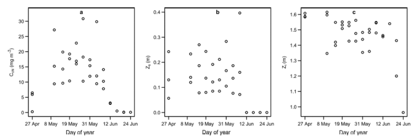
Fig. 1. Site-averaged time series plots of (a) areal concentration of Tchl a, C chl, (b) snow depth, Z s, and (c) thickness of sea ice, Z i. Z s was equal to zero during the melt, when melt ponds and drained ice replaced snow as the top of the ice cover.
Statistical analysis
Functional data analysis considers functional data arising from discrete observations of smooth functions; in this sense, the fundamental unit of observation for FDA is a curve. The goals of FDA are similar to those of more traditional statistical analyses, and include data representation and visualization, as well as the study of important sources of patterns and variation within the data. Functional versions of analysis of variance, multiple regression analysis and principal components analysis are readily available. A recurring theme in FDA is the use of information in the derivatives of functions. Several FDA methods have readily been implemented in state-of-the-art software (e.g. MATLAB® and R (Reference Ramsay and SilvermanRamsay and Silverman, 2005; Reference Ramsay and KotzRamsay, 2006; Reference Ramsay, Wickham and GravesRamsay and others, 2009; Reference R CoreR Core Team, 2013)).
In the study of environmental processes, functional data are often produced as collections of discrete measurements. The measurements within each collection usually possess a high-resolution and a low-noise component and are sometimes interpolated with the aim of characterizing an underlying smooth function that best describes the data. In general, the underlying function is defined over a continuous domain. For longitudinal data, such as temperature or precipitation time series, the domain is time, and in the case of spectral irradiance the domain is wavelength. If the measurements are made without error, then the function can be recovered via interpolation. However, observational error and natural variability in environmental (i.e. snow, ice and ice algal) properties are often present, so the recovery of the underlying function is improved via smoothing techniques.
Smoothing τ(λ)
In our study, we considered discrete measurements of incident and transmitted irradiance at several hundred wavelengths to obtain optical depth measurements of the form yl 1,yl2, ...,yln, where l is used to index snow depth site and n is the number of wavelength measurements. For each site, l, the measurement ylj equates to an optical depth τ 1 (λj) at the specific wavelength λj, for j — 1,2, . . ., n. Each optical depth curve, τ 1 (λ), was reconstructed as a regression spline (Reference Ramsay and SilvermanRamsay and Silverman, 2005), and in our application we considered B-splines of order 6 with knots placed every 2 nm. To reduce observational error, we used the roughness penalty approach to construct the regression splines for each optical depth curve. This method imposed additional smoothness by restricting the size of the third-order derivatives of the curves. Smoothing was controlled through a smoothing parameter, which was chosen to minimize the generalized cross-validation criterion (Reference Craven and WahbaCraven and Wahba, 1978). In our application, the third derivative of τ 1 (λ) was penalized using a smoothing parameter of 10-0.75
Functional regression model for τ(λ)
The Arctic ice cover was treated as a vertical arrangement of three distinct layers: a top layer of seasonally varying composition, a middle layer of sea ice with thickness Zi (m) and a bottom layer of algal biomass. For this bottom layer, C chl was the areal concentration of Tchl a (mgm–2).
The top layer consisted of snow of depth Z s (m) from 27 April to 6 June 2011. During this interval, shortwave albedo remained approximately constant at 0.84 (Reference GalindoGalindo and others, 2014). After 6 June, melt progressed, followed by a sharp decline in shortwave albedo, resulting in a surface ice cover of drained white ice interspersed with melt ponds (Reference Campbell and GosselinCampbell and others, 2014; Reference Landy, Ehn and ShieldsLandy and others, 2014). The observed depths of the drained ice layer above the water table (referred to as white ice; Reference GrenfellMaykut and Grenfell, 1975) and melt ponds were small, having maxima of 0.10 and 0.06 m, respectively. The drop in albedo associated with surface covers of these types had a significant influence on optical depth. Measurements made during the melt were few in number relative to the entire dataset, but critical for capturing the full range of C chl (i.e. C chl approached 0 m g m–2 during the melt progression; Reference Campbell and GosselinCampbell and others, 2014). Because the top layer of the ice cover was devoid of actual snow during this time, we set Z s to zero for these observations (Fig. 1 shows site-averaged time series plots of C chl, Z s and Zi).
Functional regression was used to link spectral optical depth to the scalar covariates, C chl, Z s and Zi. This technique is an extension of traditional regression to the case where either the dependent or the independent variables are functional. In our setting, the functional response was τ(λ) with A restricted to PAR, as mentioned above. The functional linear regression model we used for τ(λ) was of the form
where the dimensionless function, ∊(λ), represents a mean zero stochastic error process. The functional regression coefficients are interpreted as attenuation coefficients. Specifically, d, chl (λ) is the Tchl a-specific diffuse attenuation coefficient (m2 mg–1), and Kds(λ) and Kd,i(λ) are the spectral diffuse attenuation coefficients (m–1) of snow and ice, respectively. The intercept function, P 0 (λ) (dimensionless), represents effects on optical depth not accounted for by the covariates, including reflection and scattering due to impurities in the ice. A functional regression coefficient with a value of 0 at a given wavelength implies that its corresponding covariate has no effect on τ(λ) at that wavelength. Reference Smith, Anning and mentSmith and others (1988) used a non-functional equation of the same form to model photon fluence rate (μmol quanta m-2 s-1).
The regression coefficients, Kd,s(λ), Kd,i(λ) and K* d,chl(λ), and intercept term, β0(X), were expressed using order 6 B-spline bases with knots placed every 4nm. Fitting was accomplished by minimizing the regularized integrated residual sum of squares (Reference Ramsay and SilvermanRamsay and Silverman, 2005). A smoothing parameter of 10 2 was applied to the third derivatives of the coefficient functions, chosen to minimize the cross-validated integrated squared error (Reference Ramsay, Wickham and GravesRamsay and others, 2009). All analyses were performed using the ‘R environment for statistical computing’. Functional regression fitting and statistical analyses (confidence intervals for regression coefficients, goodness-of-fit and significance testing) were conducted with the help of the fda package (Ramsay and others, 2012). The R code and coefficient estimates used are available upon request from the authors.
Results and Discussion
Attenuation coefficients
The confidence intervals of K* d,chl(λ), (Fig. 2b-d) did not include 0 at any wavelength, except for over the wavelength range 690-700 nm. Hence, there is evidence to suggest that Tchl a, snow depth and ice thickness affect optical depth over almost all of the PAR range. Contrastingly, the zero value was included in the confidence interval of the intercept term, β0(X), at every wavelength (Fig. 2a), indicating that the covariates accounted for most of the variation in the optical depth measurements. For each layer of the ice matrix, PAR-integrated attenuation coefficients were obtained by averaging the functional coefficients over PAR wavelengths, weighting by the irradiance above and below the layer in question (following Reference Ehn and MundyEhn and Mundy, 2013). The observed ranges of snow depth and ice thickness did not substantially affect the values of these coefficients.
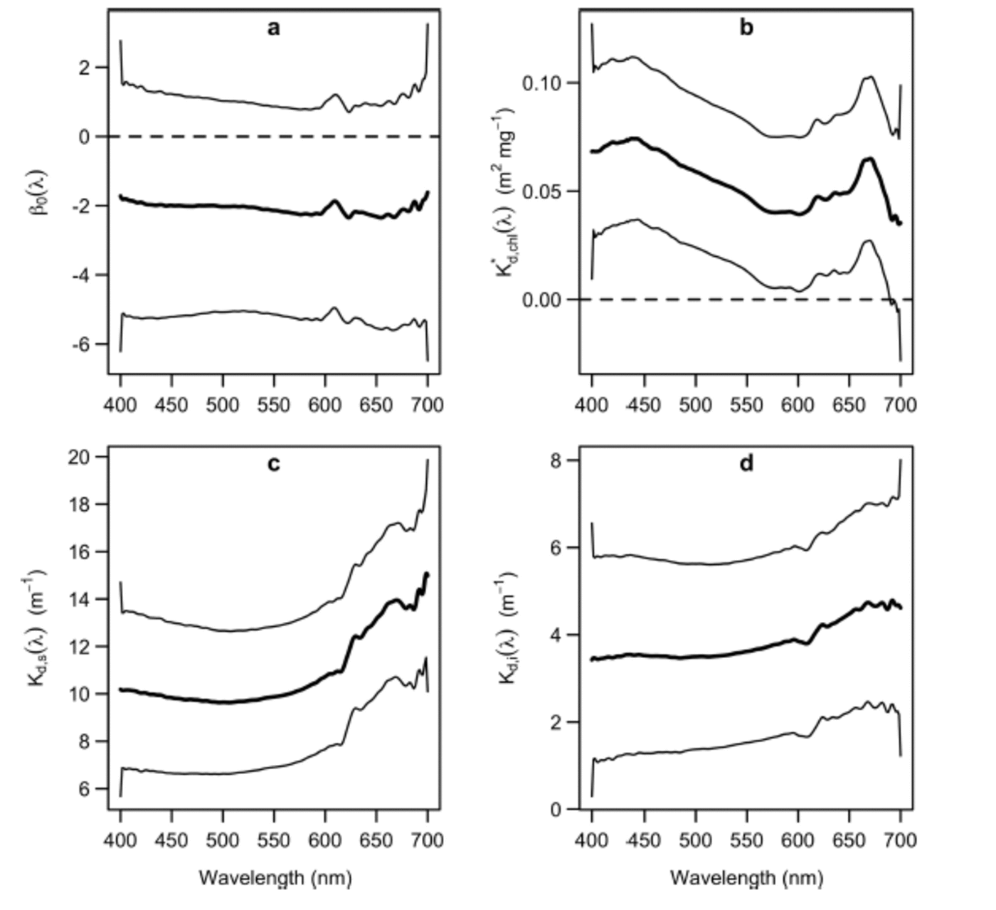
Fig. 2. Estimated coefficient functions (thick solid curves) and associated 95% confidence intervals (thin solid curves) of the functional regression model (Eqn (2)): (a) functional intercept; (b) Tchl a-specific diffuse attenuation coefficient; (c) attenuation coefficient of snow; and (d) attenuation coefficient of ice.
The shapes of K* d,chl(λ) and Kd,s (λ) were in agreement with published results: K* d,chl(λ) had peaks at ˜440 and 670nm (Reference Perovich, Cota, Maykut and GrenfellPerovich and others, 1993; Reference Mundy, Ehn, Barber and MichelMundy and others, 2007) and Kd,s (λ) had a characteristic J shape (Reference MaykutGrenfell and Maykut, 1977). Although the shape of K* d, chl(λ) was in agreement with the Tchla-specific absorption spectrum, it was higher by an offset of ∼0.05 m2 mg –1 relative to that of Reference Ehn and MundyEhn and Mundy (2013). Thus, it is likely that the total attenuation per unit of Tchla includes a scattering effect associated with algae embedded within the ice matrix (Reference Ehn, Mundy and BarberEhn and others, 2008a; Reference Ehn and MundyEhn and Mundy, 2013). The PAR-integrated Tchla-specific attenuation coefficient, K*d,chl(PAR), was 0 . 0 6 m2 mg –1, substantially larger than the 0.035 m2 mg –1 estimated by Reference Smith, Anning and mentSmith and others (1988). It is noteworthy that Reference Smith, Anning and mentSmith and others (1988) observed an increase in their K*d,chl(PAR) estimate when an outlying Tchl a measurement of 110 mg m –2 was removed from their regression. This led them to suggest that K*d,chl(PAR) might decrease with increasing Tchl a. Such a relationship would be consistent with the influence of an intercellular package effect on K*d,chl(PAR), i.e. less Tchla in the ice would increase the absorption efficiency per Tchla, due to less intercellular self-shading. We note that our maximum range of Tchla (30.85 mg m –2) was approximately one-quarter that used in the regression of Reference Smith, Anning and mentSmith and others (1988), in which the maximum Tchla value was ∼120mg m –2. Therefore, such an intercellular package effect could help to explain our higher K d*,chl(PAR) estimate.
The magnitude of Kd,s(λ) fell between the dry and melting snow coefficients summarized by Reference PerovichPerovich (1990), and its PAR-integrated value was 11 m 1, which fell within the range of values observed at a nearby location and a similar time of year by Reference Mundy, Barber and MichelMundy and others (2005). Contrastingly, the magnitude of Kd,i(λ) was slightly larger than the interior white ice and cold blue ice attenuation coefficients given by Reference PerovichPerovich (1990), with a PAR-integrated value of 3.6 m 1 . This difference could be in part attributed to the greater scattering associated with the surface granular and drained white ice layers, and the bottom skeletal ice layers of a first-year ice cover (Reference Ehn and PapakyriakouEhn and others, 2008b). Furthermore, Kd,i(λ) deviated from an expected J shape (Reference GrenfellGrenfell and Maykut, 1977), with a small secondary peak in the wavelength range ∼440nm, close to the main absorption peak of Tchl a. Therefore, the model appeared to attribute a small algal biomass influence on optical depth to sea ice. This slight effect could be attributed to variability in Tchl a concentration above the bottom 0.03 m layer, i.e. above the portion of ice where Tchl a measurements were derived.
We note that all of the coefficients had slight edge effects. For instance, K d,s(λ) experienced a local minimum at ∼690nm (Fig. 2c). Much of this variation could be due to statistical noise. Nevertheless, the level of consistency that the regression coefficients exhibited with previously established results is promising, given the inherent uncertainty in their statistical estimation.
Summary statistics
The functional coefficient of variation, R2 , and F-statistic (Reference Ramsay and SilvermanRamsay and Silverman, 2005) were used to assess model fit (Fig. 3). A permutation F-test was used to test the hypothesis that the covariates C chl, Z s and Zi had no effect on optical depth. The observed functional F-statistic was well above the 1 % critical value (Fig. 3a), leading to the conclusion that the model provided sufficient evidence that areal Tchl a concentration, snow depth and ice thickness had a statistically significant effect on optical depth over the PAR range. In addition, the functional R2 statistic varied from ∼75% to 84.5% over the PAR range (Fig. 3b). Hence, at every value of A, most of the variation in τ(λ) was explained by the model.

Fig. 3. (a) Functional F-statistic (solid curve) for a predictive relationship between Tchl a concentration, snow depth, ice thickness and spectral optical depth at each wavelength in the PAR range. The 1 % critical value of the null distribution (dashed line) is displayed at the bottom. (b) The functional coefficient of variation, R 2for the model as a function of wavelength. (Reference Perovich, Cota, Maykut and GrenfellPerovich and others, 1993; Reference Mundy, Ehn, Barber and MichelMundy and others, 2007) and Kd,s(λ)
It is significant to note that the R2 statistic had features in common with both K d,s(λ) and K*d,chl(λ), including peaks around 440 and 670 nm, a minimum at ∼575nm and a general trend of decrease from 450 to 550 nm followed by a sharp increase from 575 to 670 nm (Fig. 2b and c). The shape of the R2 curve therefore suggests that the ability of the model to explain variation in the optical depth data is directly related to the attenuation caused by the covariates included in the model.
Prediction of optical depth and transmitted irradiance
Using a measured incident irradiance spectrum from the original dataset, the estimated regression coefficients from our model and a variety of covariate values, we calculated several transmitted irradiance spectra according to

We compared low (0.06 m) and high (0.4 m) snow depths, Z s, to low (0.05 mg m 2 ) and high (30.0 mg m– 2 ) Tchla concentrations, C chl. These values approximately corresponded to the observed nonzero range of each covariate (Fig. 1). Zi was set to 1.47 m, the mean value of ice thickness for our dataset. A schematic representation of these calculations is presented in Figure 4. Not surprisingly, transmitted irradiance spectra (Fig. 4c-f) were at least one order of magnitude smaller than the incident spectrum (Fig. 4a). Increasing snow depth caused an upward vertical shift in optical depth, whereas increasing Tchla concentration caused a similar vertical shift, as well as a change in the spectral shape (Fig. 4b). In particular, the optical depth curves corresponding to high Tchla concentrations exhibited similar peaks to those of K*d,chl(λ), whereas those corresponding to low Tchl a concentrations had shapes that more closely resembled Kd,s(λ). The effects of snow and Tchla on τ(λ) were reflected in the corresponding transmitted irradiance curves (Fig. 4c-f). Increasing snow depth caused the transmitted irradiance spectra to decrease in magnitude, while approximately maintaining their shape and peak structure (Fig. 4c-f). Increasing Tchla concentration caused smaller changes in magnitude, but also changed the shapes of the spectra: low Tchl a spectra exhibited maxima in the mid-400s to early 500s, while high Tchla spectra were low in the late 400s relative to their peaks in the late 500s (Fig. 4c-f). These results are consistent with the dominance of the attenuation properties of snow and Tchla by scattering and absorption, respectively (Reference Mundy, Ehn, Barber and MichelMundy and others, 2007).

Fig. 4. (a) Spectral irradiance incident on an Arctic ice cover. (b) A sample of optical depth curves corresponding to low snow depth and low Tchla (solid curve), high snow depth and low Tchl a (thin dashed curve), low snow depth and high Tchla (dotted curve) and high snow depth and high Tchl a (thick dashed curve). (c–f) Transmitted irradiance spectra corresponding to the optical depth curves in (b).
Conclusions
Our functional linear regression model provided statistically significant evidence of the individual effects of ice algae biomass, snow and ice on optical depth, in addition to providing strong evidence of an overall predictive relationship. Furthermore, the model explained 75-84.5% of the variation in the values of the observed τ(λ) curves, and was used to predict transmitted irradiance. Although the inherent optical properties of the covariates were not explicitly accounted for in the model, their estimated effects on optical depth were largely consistent with expected results from previous work.
Unlike more comprehensive radiative transfer models (e.g. Reference PerovichPerovich, 1990; Reference Hamre, Gerland and StamnesHamre and others, 2004; Reference Ehn, Mundy and BarberEhn and others, 2008a,Reference Ehn and Papakyriakoub), our model did not require any prior assumptions of the Arctic ice cover’s optical properties. Using only a relatively small dataset, consisting of measurements of Tchla concentration, snow depth, ice thickness and irradiance, we successfully estimated spectral attenuation coefficients for each defined layer of the ice cover. Although our model’s treatment of the ice cover is not as detailed as those of the aforementioned radiative transfer models, its strong performance and agreement with previous results indicate that it provides a relatively simple way to independently estimate the effects of covariates on spectral optical depth and to verify the legitimacy of these effects. More generally, it shows that FDA can be used to model relationships, estimate quantities and validate previous results in the Arctic marine ecosystem in a straightforward and versatile way. The use of statistical methods also allows for rigorous scrutiny of results through significance testing and error analysis.
Future work will involve refinements to the model presented here, which was limited in its treatment of factors such as reflectance by the simplicity of the dataset. We will also attempt to use similar FDA techniques to predict chl a concentrations using transmitted spectral irradiance measurements. Using such techniques in conjunction with irradiance measurements made by ROVs across wide spatio-temporal regions (e.g. Reference Nicolaus and KatleinNicolaus and Katlein, 2013) would facilitate large-scale, non-destructive estimation of algal biomass, a critically important contribution considering the destructiveness and difficulty associated with direct algal measurements (Reference Mundy, Ehn, Barber and MichelMundy and others, 2007). Furthermore, we will explore the possibility of analysing changes in the Arctic ice cover’s optical properties over time by applying our models to similar datasets taken from Resolute Passage in different years and comparing the estimated coefficients. These uses of functional data analysis provide the potential for crucial new insights into the changing Arctic ice cover and marine ecosystem.
Acknowledgements
This work was supported by funding from the Natural Sciences and Engineering Research Council of Canada, Canada Economic Development and Polar Continental Shelf Program of Natural Resources Canada. We thank Mélanie Simard and Joannie Charette for the HPLC pigment analysis. This is a contribution to the research programs of ArcticNet, Arctic Science Partnership (ASP) and the Canada Excellence Research Chair unit at the Centre for Earth Observation Science.


